Modeling the RXTE light curve of $\eta$ Carinae from a
3-D SPH simulation of its binary wind collision

Abstract

The very massive star system $\eta$ Carinae exhibits regular 5.54-year (2024-day) period disruptive events in wavebands ranging from the radio to X-ray. There is a growing consensus that these events likely stem from periastron passage of an (as yet) unseen companion in a highly eccentric ($\epsilon\sim 0.9$) orbit. This paper presents three-dimensional (3-D) Smoothed Particle Hydrodynamics (SPH) simulations of the orbital variation of the binary wind-wind collision, and applies these to modeling the X-ray light curve observed by the Rossi X-ray Timing Explorer (RXTE). By providing a global 3-D model of the phase variation of the density of the interacting winds, the simulations allow computation of the associated variation in X-ray absorption, presumed here to originate from near the apex of the wind-wind interaction cone. We find that the observed RXTE light curve can be readily fit if the observer’s line of sight is within this cone along the general direction of apastron. Specifically, the data are well fit by an assumed inclination $i=45^{\circ}$ for the orbit’s polar axis, which is thus consistent with orbital angular momentum being along the inferred polar axis of the Homunculus nebula. The fits also constrain the position angle $\phi$ that an orbital-plane projection makes with the apastron side of the semi-major axis, strongly excluding positions $\phi<9^{\circ}$ along or to the retrograde side of the axis, with the best fit position given by $\phi=27^{\circ}$. Overall the results demonstrate the utility of a fully 3-D dynamical model for constraining the geometric and physical properties of this complex colliding-wind binary system.

1 Introduction

$\eta$ Carinae is one of most remarkable star systems in the galaxy. Its extreme luminosity, estimated today at some $5\times 10^{6}L_{\odot}$, implies a massive ($M>100M_{\odot}$) primary star very close to the Eddington limit. One of the most extreme examples of the class of Luminous Blue Variable (LBV) stars, its historical light curve shows irregular brightenings, the greatest of which occurred in the 1840’s, when its luminosity is estimated to have approached $25\times 10^{6}L_{\odot}$. This was accompanied by the ejection of some 10-20 $M_{\odot}$, forming what is seen today as the bipolar Homunculus nebula. In general, $\eta$ Carinae is a key object in our understanding of the formation and evolution of extremely massive stars (see, e.g., Davidson & Humphreys, 1997).

An important advance in the observational study of $\eta$ Carinae came from the identification of periodic, near-IR variations (Whitelock et al., 1994; Damineli, 1996) that are stable over many decades, along with correlated variability in the radio (Duncan et al., 1995) and X-ray (Corcoran et al., 1995) wavebands. The variability is especially dramatic in the 2-10 keV X-ray band, where the spatially unresolved X-ray flux drops by about a factor of 100 for 3 months, as shown by daily monitoring with the Rossi X-Ray Timing Explorer (RXTE) during the X-ray minimum of 1997-1998 (Ishibashi et al., 1999), and again during the 2003 X-ray minimum (Hamaguchi et al., 2007). The top panel of figure 1 compares the RXTE lightcurve vs. phase over the two full orbital cycles for 1996-2001 and 2002-2007 (Corcoran, 2005).

Analysis of this X-ray emission and light curve has provided important clues about the likely general nature of the system. First, the relative hardness of the X-rays suggests they must originate from the post-shock regions of a relatively fast wind ($\sim 3000\,{\rm km\,s^{-1}}$) from an otherwise unseen companion star, confined by the much denser, but slower ($\sim 500-800\,{\rm km\,s^{-1}}$) wind from the primary (Pittard et al., 1998; Corcoran et al., 2001; Pittard & Corcoran, 2002). The sharpness of the ingress and egress suggests moreover that the X-ray emission source must be relatively compact, probably originating mostly just inside the stagnation point of the wind-wind shock cone, along the line between the stars. And given the very high density of the primary wind, the detection of X-rays during most of the period suggests an observer perspective that looks through a relatively transparent cavity carved out by the relatively low-density secondary wind (Corcoran, 2005).

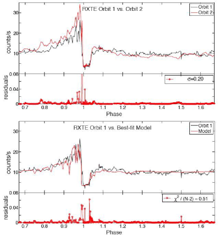
Figure 1: Top: RXTE light curve vs. orbital phase, comparing data from the first (black) and second (red) orbital periods. Bottom: Comparison of the initial orbit RXTE light-curve (black) with our best-fit model (red), with observer position angles $i=45^{\circ}$ and $\phi=27^{\circ}$, as marked by “X” in the $\chi^{2}$ contour plots in figure 4. For both comparisons, the lower boxes plot the square residuals of the fit, normalized so that the sum equals 1.

A key hindrance to moving beyond this general picture has been the lack of a 3-D hydrodynamical wind-interaction model that fully accounts for the orbital motion, which can be especially important for the sharp variations near periastron. The present paper applies Smoothed Particle Hydrodynamics (SPH) simulations to provide such a 3-D model throughout the full elliptical orbit of the binary components (Okazaki et al., 2008). For simplicity, the initial simulations here assume isothermal flow with a fixed common temperature for both winds. As such they do not directly model the shock-heated gas that is the cause of the X-ray emission. But the simulations do provide a fully 3-D, time-dependent description of the relatively cool material that is the source of X-ray absorption. By assuming a simple point-source model for the X-ray emission, located just within the head of the wind-wind shock interaction front (see figure 3), the model allows computation of the phase-variable X-ray attenuation, and thus X-ray light curve, for any assumed observer position. As detailed below, with quite nominal binary wind parameters adopted from previous analyses, the overall model, once adjusted to an optimal viewing angle, reproduces the observed RXTE light curve remarkably well (see figure 1).

Table 1: Stellar, wind, and orbital parameters

Parameters	$\eta$ Car A	$\eta$ Car B
Mass ($M_{\odot}$)	90	30
Radius ($R_{\odot}$)	90	30
Mass loss rate ($M_{\odot}\,{\rm yr}^{-1}$)	$2.5\times 10^{-4}$	$10^{-5}$
Wind velocity (${\rm km\,s}^{-1}$)	500	3,000
Wind temperature (K)	$3.5\times 10^{4}$	$3.5\times 10^{4}$
Orbital period $P$ (d)	2,024
Orbital eccentricity $e$	0.9
Semi-major axis $a$ (AU)	$15.4$

2 Model Specifications

The simulations presented here were performed with a 3-D SPH code based on a version originally developed by Benz et al. (1990) and Bate et al. (1995). Using a variable smoothing length, the SPH equations with the standard cubic-spline kernel are integrated with individual time steps for each particle. In the implementation here, the artificial viscosity parameters are $\alpha_{\rm SPH}=1$ and $\beta_{\rm SPH}=2$.

The two winds are modeled by an ensemble of gas particles that are continuously ejected with a given outward velocity at a radius just outside each star, coasting from there without any net external forces, effectively assuming that gravity is canceled by radiative driving terms. Perhaps more significantly, the simulations also assume both winds to be isothermal, with a common “warm” temperature. (The specific temperature, set to be comparable to the stellar effective temperature $T=35,000$ K, has little effect on the flow dynamics or X-ray absorption.) This is a serious simplification, made to bypass the need to resolve the complex cooling regions near the wind shocks, which is generally difficult in a 3-D model, particularly with an inherently viscous method like SPH. While this does allow a quite realistic account for the 3-D absorption by radiatively cooled material, it means that the expected X-ray emission from shock heating must be added separately (see §4).

In a standard $xyz$ Cartesian coordinate system, we set the binary orbit in the $x$-$y$ plane, with the origin at the system centre of mass, and semi-major axis along the x-axis (see figure 3). The outer simulation boundary is set at a radial distance $r=10.5a$ from the origin, where $a$ is the semi-major axis of the binary orbit. Particles crossing this boundary are removed from the simulation. By convention, we define $t=0$ (and zero phase) to be at periastron passage. Table 1 summarizes the stellar, wind, and orbital parameters, largely adopted from those derived previously by Corcoran et al. (2001) and Hillier et al. (2001). A key parameter for the global form of the wind interaction is the ratio $\eta$ of wind momentum ${\dot{M}}v$ between the primary to secondary wind, which here has a value $\eta\approx 4.2$. Simple ram pressure balance then implies that, for a binary separation $D$, the interface should be located at a distance $d=D/(1+\sqrt{\eta})\approx 0.33\,D$ from the secondary star (Stevens et al., 1992; Canto et al., 1996).

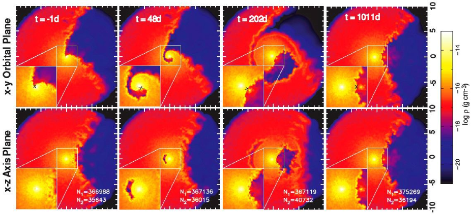
Figure 2: Snapshots of 3-D SPH simulation of wind-wind collision at times that, from left to right, are -1, +48, +202, and +1,011 days from periastron. The color scale shows the density (on a logarithmic scale with cgs units) in the $x$-$y$ orbital plane (top) and in the $x$-$z$ perpendicular plane containing the orbital and major axes (bottom). The main figures are for a square region $\pm 10a$ about the system centre of mass, while the lower-left insets show a factor two magnification of the inner $\pm 2a$; this shows more clearly the interaction front where the X-ray source is assumed located, marked by an X between the brighter and dimmer spots that represent the primary and secondary stars, within the apex of the lower density wind. Annotations give the time (in days) from periastron passage and the number of particles ($N_{1},N_{2}$) in the primary and secondary winds.

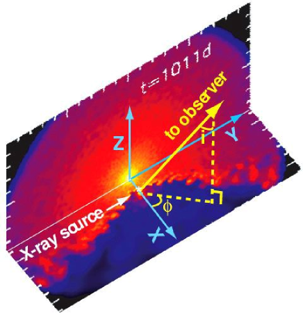
Figure 3: Schematic to illustrate observer position defined by inclination angle $i$ to the orbital axis $z$, and by equatorial projection angle $\phi$ relative to major axis $x$. The background orthogonal planes represent slices of density from our 3-D SPH simulation, shown here near apastron ($t=1011$ d) for both the $x$-$y$ orbital plane and the $y$-$z$ plane orthogal to the major axis. The X-ray source is assumed to be just inside the head of the bow front, at a distance $0.25D$ from the secondary, where $D$ is the current binary separation. The observer direction shown is roughly consistent with that inferred by the best-fit model to the RXTE lightcurve. Note that, in the conventional notation of binary orbits, using a reference plane perpendicular to the line of sight, the “argument of periapsis” $\omega=270^{\circ}-\phi$.

3 Phase variation of colliding winds

Figure 2 illustrates SPH simulation results for the density at 4 phases from near periastron (left) to near apastron (right), plotted in both the orbital plane ($x$-$y$; top row), and the perpendicular plane through the orbital and major axes ($x$-$z$; bottom row). Although instabilities in the wind-wind interaction lead to substantial stochastic variations and clumping, one can still see quite vividly how the lower-density, faster wind from the secondary carves out a cavity in the higher-density, slower wind from the primary. Throughout most of the period centered around apastron, this cavity has a relatively simple, 2-D axisymmetric, conical form similar to the apastron snapshot at $t=1011$ d, with a fixed opening half-angle $\alpha\approx 60^{\circ}$. This is in good agreement with 2-D analytic (Canto et al., 1996) and numerical models (Pittard & Corcoran, 2002) that ignore orbital motion, which near apastron is indeed small (ca. $~{}20~{}{\rm km\,s}^{-1}$) compared to the flow speed of either wind.

But near periastron, the faster variation, closer separation, and higher orbital speed (up to $\sim 360~{}{\rm km\,s}^{-1}$) all work to distort the structure. In the approach up to periastron, the 2-D interface first starts to bend, but then, as the secondary whips around the opposite side of the primary, the secondary wind cavity becomes fully enshrouded by the denser, primary wind. Over time, the segment of this shell expanding toward apastron dissipates, and the nearly 2-D axisymmetric structure is again recovered.

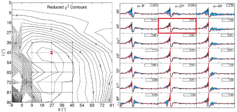
Figure 4: Left: Contours of reduced chi-squared, $\chi^{2}/(N-2)$, for deviations between RXTE lightcurve for orbit 1 and models with observer inclination angle $i$ and prograde angle $\phi$, plotted for a model grid with $9^{\circ}$ increments in both $i$ and $\phi$. The large “X” denotes the best-fit model plotted in figure 1. Right: Mosaic of lightcurves for inclinations and azimuths denoted by dots within the box bracketing the broad $\chi^{2}$ valley on left. The curves compare model (red) vs. orbit 1 RXTE data (black), with the difference shaded in cyan. The box in each panel gives the reduced chi-squared value. The red box highlights the best-fit model, with $i=45^{\circ}$, $\phi=27^{\circ}$, and $\chi^{2}/(N-2)=0.51$.

4 Modeling the RXTE light curve for $\eta$ Car

To illustrate the diagnostic potential of this 3-D SPH simulation, we now use it to model the X-ray light curve observed by RXTE. The solid black curve in figure 1 shows this light curve for the years 1996-2007, covering the two initial full periods spanning both the 1998 and 2003.5 minima (Corcoran, 2005). While the sharpness of the drop to these minima seems suggestive of an eclipse-like event, the overall asymmetry does not fit the normal form of a stellar eclipse. The pre-event rise can likely be attributed to the $1/D$ scaling of the shock emission with the declining binary separation distance $D$ toward periastron. But it is been a subject of debate whether the sharp drop and lack of a symmetric post-event peak reflects some kind of quenching of the X-ray emission (Hamaguchi et al., 2007), or is mainly just due to variations in X-ray absorption.

To explore the latter possibility, we combine the variable absorption column derived from the SPH simulations with a simple point-source model for the X-ray emission. The strongest X-ray emission is expected to come from the shock of the faster secondary wind in the region just within the head of the wind-wind interaction front. In terms of the binary separation $D$, that interaction front is itself a distance $d=D/(1+\sqrt{\eta})=0.33\,D$ from the secondary. Our model thus assumes a point source of X-ray emission located along the line of separation at a fixed fractional distance from the secondary, given by $d_{x}=f_{x}\,D$, where $f_{x}<0.33$. We have explored models with $f_{x}=$ 0.20, 0.25, and 0.30, but since the results are all qualitatively similar, we focus here just on the intermediate case with $f_{x}=0.25$.

Following the expected scaling for emission by adiabatic shocks in wind-wind collisions (Stevens et al., 1992; Pittard & Corcoran, 2002), we assume the phase variation of the X-ray source brightness varies with the inverse of the current stellar separation, $L_{x}\sim 1/D$. Defining then the time-variable mass column depth from the X-ray source to the observer as $m_{o}(t)$, the model X-ray light curve takes the form,

$$L_{x,mod}(t)=\frac{A}{D(t)}e^{-\kappa m_{o}(t)}+B\,,$$ (1)

where $A$ and $B$ are normalization constants fixed to match the observed X-ray counts respectively at apastron and post-periastron minimum. Assuming a characteristic bound-free opacity $\kappa\approx 5\,{\rm cm^{2}\,g^{-1}}$ (see, e.g., fig. 5 of Antokhin et al., 2004) for the relevant RXTE energy band (2-10 keV), we then compute the phase variation of absorption from this X-ray source to trial observers over wide range of position angles. As illustrated in figure 3, this observer position is defined by the inclination $i$ to the orbital axis, and by an orbital plane projection that makes a prograde direction angle $\phi$ with the $+x$ axis direction toward apastron.

5 Varying Observer Position for Best Fit

We have computed a grid of model X-ray light curves $L_{x,mod}(t)$ vs. temporal phase $t$ for a full range of observer’s position angles $i$ and $\phi$, varying both in increments of $9^{\circ}$. The lower panel of figure 1 compares the first-orbit RXTE light curve with the resulting best-fit model, for which $i=45^{\circ}$ and $\phi=27^{\circ}$. The agreement is as good or somewhat better than the internal agreement between the first and second orbit cycles of RXTE observations, as shown by the black vs. red curves in the upper panel. In fact, the random variations in model X-rays during the general rise before periastron appear to be statistically quite similar to RXTE variations during this phase, though of course the random nature means they don’t match in detail. In the model, these variations arise entirely from changes in absorption due to clumping in the wind interaction region of the SPH simulation, suggesting then that the observed variation might likewise be due to clump absorptions rather than, e.g., increases in the temperature or emission measure of the shock X-ray emitting region (cf. Hamaguchi et al., 2007).

For each observer position we quantify the level of agreement with the first RXTE orbit by the usual statistical measure of merit,

$$\chi^{2}=\frac{1}{\sigma^{2}}\sum_{i}\left[\frac{L_{x,mod}(t_{i})}{L_{x,obs}(t_{i})}-1\right]^{2}\,,$$ (2)

where we have assumed the data can all be characterized by a common fractional mean-square deviation $\sigma^{2}$. For the RXTE data, the contribution from measurment error is relatively unimportant compared with the inherent, apparently random variations in the observed X-rays, e.g. perhaps due to wind clumping. Moreover, in figure 1 the comparison of the RXTE light curves for successive orbital periods shows a systematic change, indicating a cycle-to-cycle variation that is not accounted for in our basic model. We thus estimate the inherent deviation by computing the averge mean-square deviation between each of these first two observation cycles,

$$\sigma^{2}\approx\frac{1}{N}\sum_{i}\left[\frac{L_{x,obs}(t-P)_{i}}{L_{x,obs}(t_{i})}-1\right]^{2}\,,$$ (3)

where $L_{x,obs}(t-P)_{i}$ represents data from the second orbit shifted back by one period $P=2024$ d and interpolated onto the data times of the first cycle. Application of this procedure for the RXTE data yields an estimated relative rms error, $\sigma=0.20$.

Figure 4 plots contours of the reduced chi-squared, $\chi^{2}_{red}\equiv\chi^{2}/(N-2)$, for the most relevant subset of our model grid, with azimuth spanning a $90^{\circ}$ range from just retrograde to strongly prograde of the major axis ($-9^{\circ}<\phi<81^{\circ}$). Noting the overall north-south symmetry, the inclination spans the full range of just the northern hemisphere, $0<\phi<90^{\circ}$. The formal best-fit model, marked with an “X”, has observer position angles $i=45^{\circ}$ and $\phi=+27^{\circ}$, with a $\chi^{2}_{red}=0.51$ that is quite significantly below the unit value required for a good fit. (This suggests our derived $\sigma=0.2$ may be about a factor $\sqrt{2}$ overestimate.)

The contours also help identify the allowed range of viewing angles, though this can be difficult to quantify rigorously. A common approach (Press et al., 2007) is to define the difference in chi-squared relative to the best-fit model, which here gives

$$\Delta\chi^{2}\equiv\chi^{2}(i,\phi)-\chi^{2}_{min}=479\times(\chi^{2}_{red}-0.51)\,,$$ (4)

where $479=N-2$ represents the number ($N=481$) of data points in the first RXTE orbit, minus the two degrees of freedom ($i,\phi$) in the data fit. It turns out even models neighboring the best-fit have $\Delta\chi^{2}>10$, sometimes several tens or even in the hundreds; by formal statistics they would all be excluded at well above the 99% confidence level. Taken at face value, this implies that, around the best-fit values $i=45^{\circ}$ and $\phi=27^{\circ}$, the range in both allowed viewing angles is less than the $\pm 9^{\circ}$ of the model grid. But this approach very likely greatly overstates the real exclusion probability, given that we are fixing many model parameters about the orbit, winds, location of the X-ray source, etc.

Nonetheless, even the reduced chi-squared contours do seem to strongly exclude azimuths with $\phi<9^{\circ}$ that are near or retrograde of the major axis; likewise, inclinations near the orbital axis, i.e. with $i\leq 36^{\circ}$, seem also excluded. On the other hand, viewing angles over the broad plateau within $\chi^{2}_{red}\approx 1$ (representing a doubling of the minimum) might still be allowed. The range in azimuth ($9^{\circ}<\phi<45^{\circ}$) and inclination ($36^{\circ}<i<90^{\circ}$) essentially just places the observer on the prograde side within the wind interaction cone of half-angle $\sim 60^{\circ}$ about the apastron side of the major axis $x$ (see figure 3).

The right panel of figure 4 compares lightcurves for viewing angles that bracket this allowed region. Comparison of the relative area of cyan shading between the observed and model curves supports the view that the full range of inclination $i=45^{\circ}-81^{\circ}$ around $\phi=27^{\circ}\pm 9^{\circ}$ give an acceptably good fit, while models outside this range do not.

6 Conclusions and future work

The relative ease and natural way that the observed RXTE light curve is fit by this 3-D absorption plus point-source-emission model provides good evidence for the basic validity of the overall paradigm, the key features of which are:

1. A highly elliptical orbit with the observer viewing from the general direction of apastron and prograde of the semi-major axis, through a cavity carved out in the slower, denser, primary wind by the faster, less-dense, secondary wind.

2. A relatively localized X-ray source located on the secondary side of the interaction front between the stars.

3. The X-ray mininum arising from a “wind eclipse” of this localized source as the primary wind engulfs the secondary wind just after periastron.

Note that the last point implies that “quenching” of the X-ray emission is not likely to be a dominant effect in causing the broad-band X-ray minimum. On the other hand, recent analyses (Hamaguchi et al., 2007) suggest that some sort of spectral variation of emission may be necessary to explain observed changes in the X-ray hardness. In future work, we plan to extend our analyses to include more realistic models of the energy dependence of both the emission and absorption, with a particular focus on explaining such spectral energy and hardness variations.

Acknowledgements

A.T.O. thanks the Japan Society for the Promotion of Science for financial support via Grant-in-Aid for Scientific Research (16540218). SPH simulations were performed on HITACHI SR11000 at Hokkaido University Information Initiative Center. S.P.O. acknowledges support of NSF grant AST-0507581 and NASA grant Chandra/TM7-8002X. C.M.R. acknowledges support of a NSF GK-12 fellowship. MFC acknowledges support from NASA and the RXTE program. We thank D. Cohen for many helpful comments.

References

- Antokhin et al. (2004) Antokhin, I. I., Owocki, S. P., & Brown, J. C. 2004, ApJ 611, 434
- Bate et al. (1995) Bate M.R., Bonnell I.A., Price N.M. 1995, MNRAS 285, 33
- Benz et al. (1990) Benz W., Bowers R.L., Cameron A.G.W., Press W.H. 1990, ApJ 348, 647
- Canto et al. (1996) Canto, J., Raga, A. C., & Wilkin, F. P. 1996, ApJ 469, 729
- Corcoran et al. (1995) Corcoran, M. F., Rawley, G. L., Swank, J. H., & Petre, R. 1995, ApJ 445, L121
- Corcoran et al. (2001) Corcoran, M.F., Ishibashi, K., Swank, J.H., & Petre, R. 2001, ApJ 547, 1034
- Corcoran (2005) Corcoran, M.F. 2005, AJ 129, 2018
- Damineli (1996) Damineli, A. 1996, ApJ 460, L49
- Davidson & Humphreys (1997) Davidson, K., & Humphreys, R. M. 1997, Ann.Rev.Ast.As 35, 1
- Duncan et al. (1995) Duncan, R. A. et al. 1995, Revista Mexicana de Astronomia y Astrofisica Conference Series, 2, 23
- Hamaguchi et al. (2007) Hamaguchi, K., et al. 2007, ApJ 663, 522
- Hillier et al. (2001) Hillier, D.J., Davidson, K., Ishibashi, K., & Gull, T. 2001, ApJ 553, 837
- Ishibashi et al. (1999) Ishibashi, K. et al. 1999, ApJ 524, 983
- Okazaki et al. (2008) Okazaki, A.T., Owocki, S.P., Russell, C.M.P., & Corcoran, M.F. 2008, In: Massive Stars as Cosmic Engines, IAU Symp. 250, F. Bresolin, P. Crowther & J. Puls, eds., ASP Conf. Ser., in press.
- Press et al. (2007) Press, W. H., Teukolsky, S. A., Vetterling, W. T., and Flannery, B. P. 2007, Numerical Recipes, 3rd ed., Cambridge Univ. Press.
- Pittard et al. (1998) Pittard, J. M., Stevens, I. R., Corcoran, M. F., & Ishibashi, K. 1998, MNRAS 299, L5
- Pittard & Corcoran (2002) Pittard, J. M., & Corcoran, M. F. 2002, A&A 383, 636
- Stevens et al. (1992) Stevens, I. R., Blondin, J. M., & Pollock, A. 1992, ApJ 386, 265
- Whitelock et al. (1994) Whitelock, P. A., Feast, M. W., Koen, C., Roberts, G., & Carter, B. S. 1994, MNRAS 270, 364