Entangled photon pairs from a quantum dot cascade decay:
the effect of time-reordering

Abstract

Coulomb interactions between confined carriers remove degeneracies in the excitation spectra of quantum dots. This provides a which path information in the cascade decay of biexcitons, thus spoiling the energy-polarization entanglement of the emitted photon pairs. We theoretically analyze a strategy of color coincidence across generation (AG), recently proposed as an alternative to the previous, within generation (WG) approach. We simulate the system dynamics and compute the correlation functions within the density-matrix formalism. This allows to estimate quantities that are accessible by a polarization-tomography experiment, and that enter the expression of the two-photon concurrence. We identify the optimum parameters within the AG approach, and the corresponding maximum values of the concurrence.

I Introduction

In view of their peculiar level structure, semiconductor quantum dots (QDs) are considered promising sources on demand of entangled photon pairs. Benson et al. (2000); Stace et al. (2003) Although alternative strategies have been envisaged, based on the use of single-photon sources and postselection, Fattal et al. (2004); Benyoucef et al. (2004) the possibility of deterministically generating frequency-polarization entangled photon pairs by a single cascade emission has recently received strong experimental support. Akopian et al. (2006); Stevenson et al. (2006); Young et al. (2006) There, the radiative relaxation of the dot from the lowest biexciton level generates a two-photon quantum state: $|\psi_{ph}\rangle=(|\phi_{H};H,H\rangle+|\phi_{V};V,V\rangle)/\sqrt{2}$, where $H$ and $V$ are the two linear polarizations, whereas $|\phi_{H}\rangle$ and $|\phi_{V}\rangle$ refer to the spectral degrees of freedom. In particular, $|\phi_{H}\rangle$ ($|\phi_{V}\rangle$) is the wavepacket resulting from the sequential emission of two photons, with central frequencies $\omega_{p}$ and $\omega_{r}$ ($\omega_{q}$ and $\omega_{s}$) (Fig. 1). Ideally, $\omega_{1}\!\equiv\!\omega_{p}\!=\!\omega_{q}$ and $\omega_{2}\!\equiv\!\omega_{r}\!=\!\omega_{s}$ (analogous equations hold for the relaxation rates): therefore, $|\psi_{ph}\rangle\!=\!(|H,H\rangle+|V,V\rangle)/\sqrt{2}\otimes|\phi\rangle$, with $|\phi\rangle\!\equiv\!|\phi_{H}\rangle\!=\!|\phi_{V}\rangle$. In realistic conditions, however, the degree of entanglement is limited by three main factors. Troiani et al. (2006); Hohenester et al. (2007); Hudson et al. (2007) First, an imperfect system excitation results in a finite probability that the system does not undergo a single cascade decay, thus emitting more (or less) than the two desired photons. Second, the coupling of the confined excitons with phonons tends to induce a loss of phase coherence in the state of the emitted photons. Third, the presence of an excitonic fine-structure splitting tends to make photons emitted with orthogonal polarizations distinguishable in the spectral domain: $\delta_{HV}\!=\!\omega_{p}\!-\!\omega_{q}\!=\!\omega_{s}\!-\!\omega_{r}\!\neq\!0$, and therefore $|\langle\phi_{H}|\phi_{V}\rangle|\neq 1$. This provides a which path information, which impedes to rotate the $H$ and $V$ components of $|\psi_{ph}\rangle$ one into another by linear optics elements and to observe interference effects between them.

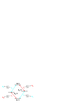
Figure 1: (Color online) Level structure of the quantum dot. The fine-structure splitting and the biexciton binding energy are given respectively by $\delta_{HV}\!\!=\!\!E_{3}\!-\!E_{2}$ and $\Delta_{B}\!\!=\!\!E_{2}+E_{3}-E_{4}$. In the WG strategy, the ideal case corresponds to the biexciton and exciton emission frequencies being independent on the polarization: $\omega_{1}\!\equiv\!\omega_{p}\!=\!\omega_{q}$ and $\omega_{2}\!\equiv\!\omega_{r}\!=\!\omega_{s}$ ($\delta_{HV}\!=\!0$). In the AG approach the photon emitted in the $B\rightarrow X_{H}$ ($B\rightarrow X_{V}$) transition matches the color of that emitted by the $X_{V}\rightarrow G$ ($X_{H}\rightarrow G$) decay ($\Delta_{B}\!=\!0$). Therefore, $\omega_{1}\!\equiv\!\omega_{p}\!=\!\omega_{s}$ (cyan arrows) and $\omega_{2}\!\equiv\!\omega_{q}\!=\!\omega_{r}$ (red arrows). In order to erase the which-path information provided by the emission order of the $\omega_{1}$ and $\omega_{2}$ photons, which is opposite in the two paths, the photons are delayed by $\delta_{\chi}$ ($\chi=p,q,r,s$).

In optimizing the entangled-photon source, part of the recent effort has been concentrated on the solution of the latter problem. Possible strategies include quenching of the excitonic fine-structure splitting $\delta_{HV}$ by means of magnetic field Stevenson et al. (2006); Young et al. (2006) or ac-Stark effect Jundt et al. (2008), and spectral filtering of the emitted photons. Akopian et al. (2006) An ingenious alternative consists in engineering the system so as to obtain color coincidence across generation (AG), rather than within generation (WG). fin ; Reimer et al. (2007); Avron et al. (2008) There, the QD spectrum is tuned in such a way to have vanishing biexciton binding energy ($\Delta_{B}=E_{2}+E_{3}-E_{4}$), so that the four emission frequencies $\omega_{\chi}$ ($\chi\!\!=\!\!p,q,r,s$) reduce to two: $\omega_{1}\!\equiv\!\omega_{p}\!=\!\omega_{s}$ (cyan arrows in Fig. 1) and $\omega_{2}\!\equiv\!\omega_{q}\!=\!\omega_{r}$ (red arrows). In the AG scheme, however, the which-path information is provided by the order in which the $\omega_{1}$ and $\omega_{2}$ photons are emitted, which is now opposite for the two polarizations. In order to make the $H$ and $V$ paths spectrally indistinguishable, the photons emitted in the four modes $\chi$ should be spatially separated and time delayed by $\delta_{\chi}$. The time reordering implements a unitary transformation ($U=U_{H}\otimes|H,H\rangle\langle H,H|+U_{V}\otimes|V,V\rangle\langle V,V|$ ) of the two-photons state, such that: $|\langle\phi_{H}|U_{H}^{\dagger}U_{V}|\phi_{V}\rangle|>|\langle\phi_{H}|\phi_{V}\rangle|$. Avron et al. (2008)

Hereafter, we investigate the viability and the limits of the AG approach. More specifically, we verify to which extent the which path information can be erased by introducing these frequency and polarization selective delays. To this aim, we derive analytic expressions for an entanglement measure (namely, the concurrence, wootters $\mathcal{C}$) of the two-photon state, and derive the expressions of the delays $\delta^{M}_{\chi}$ that maximize $C$, as a function of the emission rates $\Gamma_{\chi}$. This is the same as optimizing the unitary quantum erasure $U$ of the which-path information, for a given source. In addition, we maximize $C(\delta^{M}_{\chi})$ with respect to $\Gamma_{\chi}$, thus providing indications for the optimization of the two-photon source. In semiconductor quantum dots, the (relative) values of the exciton and biexciton relaxation rates can only be engineered within a limited range of values.Wimmer et al. (2006) However, such ranges can be potentially extended by coupling the QD to an optical microcavity. In the weak-coupling regime, the effect of the cavity on the dot dynamics essentially consists in enhancing the photon-emission rates of resonant transitions (Purcell effect). Therefore, and in order to allow analytic solutions, we don’t include the degrees of freedom of the cavity explicitly, but rather mimic its effect by enhancing $\Gamma_{\chi}$. We also neglect the effect of pure dephasing and imperfect initialization of the QD state (i.e., of realistic excitation conditions). In fact, the way in which these affect the degree of frequency-polarization entanglement is independent on the approach, AG or WG. Detailed discussions on these effects, can be found in the literature. Troiani et al. (2006); Hohenester et al. (2007); Hudson et al. (2007)

The paper is organized as follows. In Sec. II we introduce the density matrix approach we use, and the correlation functions that enter the calculation of the two-photon concurrence. Further details on the method are given in the Appendixes. In Sec. III we give the expressions of the concurrence, and maximize it with respect to the relevant parameters. In Sec. IV we draw our conclusions.

II Method

The time evolution of the dot density matrix, $\rho_{QD}$, is described by the master equation ($\hbar\!=\!1$): $\dot{\rho}_{QD}=i[\rho_{QD},H]+\sum_{\chi}\mathcal{L}_{\chi}\rho_{QD}$, where $H=\sum_{k=1}^{4}E_{k}|k\rangle\langle k|$ and $|k\rangle$ are the QD eigenstates (in the following, we take $E_{1}\!=\!0$). The radiative relaxation processes are accounted for by the four superoperators in the Lindblad form: $\mathcal{L}_{\chi}\rho_{QD}=\sigma_{\chi}\rho_{QD}\sigma_{\chi}^{\dagger}-(\sigma_{\chi}^{\dagger}\sigma_{\chi}\rho_{QD}+\rho_{QD}\sigma_{\chi}^{\dagger}\sigma_{\chi})/2$, with $\chi=p,q,r,s$. Each of the ladder operators $\sigma_{\chi}$ corresponds to one of the optical transitions in the four-level system: $\sigma_{p}\!\equiv\!\sqrt{\Gamma_{p}}\,|2\rangle\langle 4|$, $\sigma_{q}\!\equiv\!\sqrt{\Gamma_{q}}\,|3\rangle\langle 4|$, $\sigma_{r}\!\equiv\!\sqrt{\Gamma_{r}}\,|1\rangle\langle 2|$, $\sigma_{s}\!\equiv\!\sqrt{\Gamma_{s}}\,|1\rangle\langle 3|$. The quantum dot is initialized in the biexciton state: $\rho_{QD}(0)=|4\rangle\langle 4|$; in the absence of multiple excitation-relaxation cycles, the cascade-emission process from such level results in the generation of two photons. The following time evolution of $\rho_{QD}$ can be solved analytically (see Appendix A). Within the AG approach, the photons are delayed in time by a quantity that depends on their energy and polarization (Fig. 1). The resulting relations between the input mode $\sigma_{\chi}$ and the corresponding output modes $a_{\alpha i}$ read (up to a common time delay):

$$a_{H1}(t)=\sigma_{p}(t-\delta_{p}) a_{H2}(t)=\sigma_{r}(t-\delta_{r}),$$ ,

$$a_{V1}(t)=\sigma_{s}(t-\delta_{s}) a_{V2}(t)=\sigma_{q}(t-\delta_{q}).$$ , (1)

The quantity of interest here is the degree of entanglement between the frequency and polarization degrees of freedom of the two-photon state. This can be computed from their density matrix $\rho_{ph}$ which is derived from the QD dynamics (i.e., from $\rho_{QD}$) through Eqs. (II). In the following, we refer to the basis $\{|H1,H2\rangle,|H1,V2\rangle,|V1,H2\rangle,|V1,V2\rangle\}$; here, the first (second) mode is identified by the central frequency $\omega_{1}\!\equiv\!\omega_{p}$ ($\omega_{2}\!\equiv\!\omega_{r}$), which coincides with $\omega_{s}$ ($\omega_{q}$) in the ideal case $\Delta_{B}=0$. Within a single cascade decay, and in the absence of non-radiative relaxation channels, the matrix elements of $\rho_{ph}$ correspond to the time integrals of second-order correlation functions (see Appendix B):

$$\langle\alpha 1,\beta 2|\rho_{ph}|\gamma 1,\delta 2\rangle=\int\!\!dt^{\prime}\int\!\!d\tau^{\prime}\ G_{\alpha\beta\gamma\delta}(t^{\prime},\tau^{\prime}).$$ (2)

Here, $G_{\gamma\delta\alpha\beta}(t,\tau)=G^{ij}_{\alpha\beta\gamma\delta}(t,|\tau|)$, with $ij=12$ for $\tau>0$ and $ij=21$ for $\tau<0$, whereas

$$G^{ij}_{\gamma\delta\alpha\beta}(t,\tau\!>\!0)=\langle a_{\alpha i}^{\dagger}(t)\,a_{\beta j}^{\dagger}(t\!+\!\tau)\,a_{\gamma j}(t\!+\!\tau)\,a_{\delta i}(t)\rangle.$$ (3)

After applying Eqs. (II), the second-order correlation functions involving the time-shifted ladder operators $\sigma_{\chi}$ are solved by means of the quantum regression theorem (see Appendix A). Experimentally, the matrix elements of $\rho_{ph}$ can be accessed within a polarization tomography experiment. Akopian et al. (2006); Stevenson et al. (2006); Young et al. (2006); Meirom et al. (2007)

Given the above master equation and initial conditions, only few elements of the density matrix do not vanish identically (see Appendixes). These are the diagonal elements $\rho_{HH}\equiv\langle H1,H2|\rho_{ph}|H1,H2\rangle$ and $\rho_{VV}\equiv\langle V1,V2|\rho_{ph}|V1,V2\rangle$, and the off-diagonal one $\rho_{HV}\equiv\langle H1,H2|\rho_{ph}|V1,V2\rangle$. As a consequence, the two-photon density matrix reads:

$$\rho_{ph}=\left(\begin{array}[]{cccc}\rho_{HH}&0&0&\rho_{VH}\\ 0&0&0&0\\ 0&0&0&0\\ \rho_{HV}&0&0&\rho_{HH}\end{array}\right).$$ (8)

The degree of entanglement of the two-photon state can be quantified by the concurrence ($\mathcal{C}$), whose value ranges from 0 to 1, going from factorizable to maximally entangled states. For the above density matrix, it is easily seen that $\mathcal{C}(\rho_{ph})=2|\rho_{HV}|$.

III Results

III.1 Two-photon density matrix

We start by considering the diagonal matrix elements of $\rho_{ph}$, namely $\rho_{HH}$ and $\rho_{VV}$. The contribution to $\rho_{HH}^{12}=\langle H1,H2|\rho_{ph}|H1,H2\rangle$ corresponding to the ordered detection of photons $H1$ and $H2$ is given by the time integral of the correlation function

$$G^{12}_{HHHH}(t^{\prime},\tau^{\prime}) \!=\! \langle\sigma_{p}^{\dagger}(t)\,\sigma_{r}^{\dagger}(t+\tau)\,\sigma_{r}(t+\tau)\,\sigma_{p}(t)\,\rangle$$ (9)

$$= \Gamma_{p}\Gamma_{r}\exp[-(\Gamma_{p}+\Gamma_{q})t-\Gamma_{r}\tau],$$

where $t^{\prime}\!=\!t+\delta_{p}$ and $\tau^{\prime}\!=\!\tau+\delta_{r}-\delta_{p}$. The condition that the $H1$ photon is detected before $H2$ ($\tau^{\prime}\!>0\!$) results into a lower bound for the delay in the input modes $\sigma_{\chi}$: $\tau>{\rm max}(0,\delta_{r}-\delta_{p})$. Analogously, the contribution to $\langle V1,V2|\rho_{ph}|V1,V2\rangle$ corresponding to the ordered detection of photons $V1$ and $V2$, $\rho_{VV}^{12}$, is given by the time integral of the correlation function:

$$G^{12}_{VVVV}(t^{\prime},\tau^{\prime}) \!=\! \langle\sigma_{q}^{\dagger}(t)\,\sigma_{s}^{\dagger}(t+\tau)\,\sigma_{s}(t+\tau)\,\sigma_{q}(t)\,\rangle$$ (10)

$$= \Gamma_{q}\Gamma_{s}\exp[-(\Gamma_{p}+\Gamma_{q})t-\Gamma_{s}\tau],$$

where $t^{\prime}\!=\!t+\tau+\delta_{s}$ and $\tau^{\prime}\!=\!-\tau+\delta_{q}-\delta_{s}$.

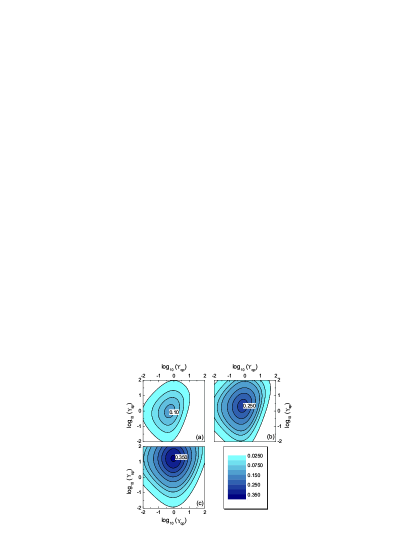
Figure 2: (Color online) Values of $|\rho_{HV}|=\mathcal{C}^{M}({\bf\Gamma})/2$ as a function of $\Upsilon_{sp}$ and $\Upsilon_{qp}$ (where $\Upsilon_{\chi\chi^{\prime}}\!\!=\!\!\Gamma_{\chi}/\Gamma_{\chi^{\prime}}$). The value of $\log(\Upsilon_{rp})$ has been fixed to $-1.2$ (a), 0 (b), and $1.2$ (c).

Here, the photon order in the output modes ($a_{V1}$ and $a_{V2}$) is inverted with respect to that of the corresponding input modes ($\sigma_{s}$ and $\sigma_{q}$). This condition results in an upper bound for the delay in the emission process: $0<\tau\!<\!\delta_{q}-\delta_{s}$.

After time integration in $t$ and $\tau$, the above expressions yeld the following coincidence probabilities:

$$\rho_{HH}^{12} \!=\! \Gamma_{p}\Gamma_{r}\int_{0}^{\infty}dt\int_{\max(0,\delta_{pr})}^{\infty}d\tau\,e^{-(\Gamma_{p}+\Gamma_{q})t-\Gamma_{r}\tau}$$ (11a)

$$\!=\! \frac{\Gamma_{p}}{\Gamma_{p}+\Gamma_{q}}\{\exp[-\Gamma_{r}\!\!\times\!\max(0,\delta_{pr})]\},$$

$$\rho_{VV}^{12} \!=\! \Gamma_{q}\Gamma_{s}\int_{0}^{\infty}dt\int_{0}^{\delta_{qs}}d\tau\,e^{-(\Gamma_{p}+\Gamma_{q})t-\Gamma_{s}\tau}$$ (11b)

$$\!=\! \frac{\Gamma_{q}}{\Gamma_{p}+\Gamma_{q}}\{1-\exp[-\Gamma_{s}\!\!\times\!\min(0,\delta_{qs})]\},$$

with $\delta_{\chi\chi^{\prime}}\!\equiv\!\delta_{\chi}-\delta_{\chi^{\prime}}$. Analogous expressions apply to the case $ij=21$. After summing up the contributions corresponding to the two cases, the diagonal elements in the two-photon density matrix take the simple form: $\rho_{HH}\!=\!\rho_{HH}^{12}+\rho_{HH}^{21}\!=\!\Gamma_{p}/(\Gamma_{p}+\Gamma_{q})$ and $\rho_{VV}\!=\!\rho_{VV}^{12}+\rho_{VV}^{21}\!=\!\Gamma_{q}/(\Gamma_{p}+\Gamma_{q})$. Even though the two-photon concurrence depends on the off-diagonal terms of $\rho_{ph}$, upper limits for $\mathcal{C}$ can already be derived from the diagonal elements. In fact, being $|\rho_{HV}|^{2}\leq\rho_{HH}\rho_{VV}$, it turns out that $\mathcal{C}\leq\mathcal{C}_{0}\equiv\!2\Upsilon_{pq}^{1/2}/(1+\Upsilon_{pq})$, with $\Upsilon_{\chi\chi^{\prime}}\!\!\equiv\!\!\Gamma_{\chi}/\Gamma_{\chi^{\prime}}$. Such upper limit, corresponding to the density matrix $\rho_{ph}$ of a pure state, has an absolute maximum of 1 for $\Upsilon_{pq}\!=\!1$. The physical interpretation of the above inequality is that, besides the erasure of the which-path information, a high degree of entanglement in the two-photon state requires a balanced branching ratio between the $H$ and $V$ decay paths.

The relevant off-diagonal matrix element of $\rho_{ph}$ is given by the time integral of the correlation functions (Eq. (2)):

$$G_{HHVV}(t^{\prime},\tau^{\prime})\!\!\! = \!\!\!\langle\sigma_{p}^{\dagger}(t)\sigma_{r}^{\dagger}(t\!+\!\tau)\sigma_{s}(t\!+\!\delta_{ps})\sigma_{q}(t\!+\!\tau-\delta_{qr})\rangle$$ (12)

$$= \exp[A(t,\tau)+iB(\tau)],$$

where $t^{\prime}\!=\!t+\delta_{p}$ and $\tau^{\prime}\!=\!\tau+\delta_{r}-\delta_{p}$. The real and imaginary parts of the exponent in the second line are:

$$A(t,\tau)\!\!\! \equiv \!\!\!A_{0}\!-\!(\Gamma_{p}\!+\!\Gamma_{q})t\!-\!(\Gamma_{p}\!+\!\Gamma_{q}\!+\!\Gamma_{r}\!-\!\Gamma_{s})\tau/2,$$ (13)

$$B(\tau)\!\!\! \equiv \!\!\!B_{0}\!-\!(E_{4}\!-\!E_{2}\!-\!E_{3})\tau,$$ (14)

where $A_{0}\!=\!(\Gamma_{p}+\Gamma_{q})\delta_{qr}/2-\Gamma_{s}(\delta_{qr}+\delta_{ps})/2$ and $B_{0}\!=\!(E_{4}-E_{2})\delta_{ps}-E_{2}\delta_{qr}$. The integration intervals result from the requirements that, in Eq. (12), all times in the input modes be positive ($t+\tau\!>\!\delta_{qr},t\!>\!-\delta_{ps}$), and that the biexciton relaxation takes place before the exciton one ($\tau\!<\!\delta_{ps}\!+\!\delta_{qr}$); otherwise the two-time expectation value on the right-hand side of Eq. (12) vanishes identically. As a consequence, the phase coherence between the two linearly polarized components of the two-photon state reads:

$$\rho_{VH}=\int_{\max(0,\delta_{ps})}^{\infty}dt\int_{\delta_{qr}-t}^{\delta_{ps}+\delta_{qr}}d\tau\ e^{A(t,\tau)+iB(\tau)}.$$ (15)

A finite biexciton binding energy would result in an oscillating term $e^{iB(\tau)}$, and therefore in a suppression of $|\rho_{HV}|$ for $|\Delta_{B}|\!\gtrsim\!(\Gamma_{p}+\Gamma_{q}+\Gamma_{r}-\Gamma_{s})/2$. Within the WG strategy, the analogous condition reads: $|\delta_{HV}|\!\gtrsim\!(\Gamma_{r}\!+\!\Gamma_{s})/2$. If the resonance condition $E_{4}\!=\!E_{2}+E_{3}$ is fulfilled, then $B(\tau)=B_{0}$, and the (constant) phase of $G_{HHVV}(t,\tau)$ plays no role. The concurrence that quantifies the energy-polarization entanglement of the two-photon state then corresponds to:

$$\mathcal{C}\!\!\!\! = \!\!\!\!\frac{2\,(\prod_{\chi}\Gamma_{\chi})^{1/2}}{CDE}\left\{C{\rm e}^{-[\Gamma_{s}\delta_{ps}+(\Gamma_{p}+\Gamma_{q}+\Gamma_{s})\delta_{qr}]/2}+\right.$$ (16)

$$D \!\!\left.\!\!{\rm e}^{-(\Gamma_{s}\delta_{ps}\!+\!\Gamma_{r}\delta_{qr})/2}\!\!+\!\!E{\rm e}^{-[\Gamma_{r}\delta_{qr}\!+\!(\Gamma_{p}\!+\!\Gamma_{q}\!+\!\Gamma_{r})\delta_{ps}]/2}\!\right\}\!\!,$$

where $C\!\!=\!\!-(\Gamma_{p}\!+\!\Gamma_{q}\!+\!\Gamma_{r}\!-\!\Gamma_{s})/2$, $E\!\!=\!\!-(\Gamma_{p}\!+\!\Gamma_{q}\!-\!\Gamma_{r}\!+\!\Gamma_{s})/2$, and $D\!\!=\!\!\Gamma_{p}\!+\!\Gamma_{q}$. We note that $\mathcal{C}$ only depends on $\delta_{ps}$ and $\delta_{qr}$, and not on the four delays $\delta_{\chi}$ independently. This is consistent with the intuition that the degree of entanglement depends on the extent to which the delays make the $H1$ ($H2$) mode indistinguishable from $V1$ ($V2$) in the time domain.

III.2 Parameter optimization

Given the analytic expression of the concurrence, $\mathcal{C}(\delta_{ps},\delta_{qr};{\bf\Gamma})$, we first maximize it with respect to the delays, as a function of the relaxation rates. The optimum values of the delays are denoted with $\delta_{ps}^{M}({\bf\Gamma})$ and $\delta_{qr}^{M}({\bf\Gamma})$, being ${\bf\Gamma}\!=\!(\Gamma_{p},\Gamma_{q},\Gamma_{r},\Gamma_{s})$. The corresponding concurrence is

$$\mathcal{C}^{M}({\bf\Gamma})\equiv\mathcal{C}[\delta_{ps}^{M}({\bf\Gamma}),\delta_{qr}^{M}({\bf\Gamma});{\bf\Gamma}].$$ (17)

In a second step, we maximize $\mathcal{C}^{M}({\bf\Gamma})$ with respect to the relaxation rate, thus identifying the absolute maximum of $\mathcal{C}$, namely $\mathcal{C}_{opt}\equiv\mathcal{C}^{M}({\bf\Gamma}_{opt})$.

The values of the relative delays that maximize $\mathcal{C}$ satisfy the conditions: $\partial\mathcal{C}/\partial\delta_{ps}=0$ and $\partial\mathcal{C}/\partial\delta_{qr}=0$. Their expressions read:

$$\delta_{ps}^{M}({\bf\Gamma})\!\! = \!\!\frac{2}{\sum_{\chi}\Gamma_{\chi}-2\Gamma_{s}}\ln\left(\frac{\sum_{\chi}\Gamma_{\chi}}{2\Gamma_{s}}\right),$$ (18a)

$$\delta_{qr}^{M}({\bf\Gamma})\!\! = \!\!\frac{2}{\sum_{\chi}\Gamma_{\chi}-2\Gamma_{r}}\ln\left(\frac{\sum_{\chi}\Gamma_{\chi}}{2\Gamma_{r}}\right).$$ (18b)

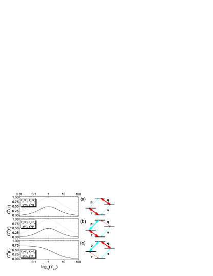
Figure 3: (Color online) The solid black lines give the values of the concurrence for optimized delays, $\mathcal{C}^{M}$, as a function of the ratio $\Upsilon_{\chi,\chi^{\prime}}=\Gamma_{\chi}/\Gamma_{\chi^{\prime}}$ and for different constraints. (a) $\Gamma_{s}=\Gamma_{p}$ and $\Gamma_{r}=\Gamma_{q}$, with $(\chi,\chi^{\prime})=(q,p)$; (b) $\Gamma_{s}=\Gamma_{q}$ and $\Gamma_{r}=\Gamma_{p}$, with $(\chi,\chi^{\prime})=(p,q)$; (c) $\Gamma_{q}=\Gamma_{p}$ and $\Gamma_{s}=\Gamma_{r}$, with $(\chi,\chi^{\prime})=(p,r)$. The dashed lines are the values of the upper limits for the concurrence $\mathcal{C}_{0}$, corresponding to a complete cancelation of the which-path information. Photon emission rates that are set equal are denoted by arrows of equal thickness in the level schemes on the right-hand side of each plot.

In the general case, one can substitute the above equations in Eq. (16), thus obtaining $\mathcal{C}^{M}({\bf\Gamma})$. In order to maximize the concurrence, we look for the values of $\Gamma_{\chi}$ that satisfy the equations: $\partial\mathcal{C}^{M}/\partial\Gamma_{\chi}=0$. No value of ${\bf\Gamma}$ simultaneously fulfils these conditions. Therefore, we numerically compute $\mathcal{C}^{M}({\bf\Gamma})$ for a wide range of relaxation-rates values: $\Upsilon_{m}<\Upsilon_{qp},\Upsilon_{rp},\Upsilon_{sp}<\Upsilon_{M}$. The global maximum of the concurrence corresponds to $\Gamma_{p}\!=\!\Gamma_{q}$ and $\Gamma_{r}\!=\!\Gamma_{s}$, with the latter rates much larger than the former ones:

$$\mathcal{C}_{opt}=\lim_{\Upsilon_{pr}\rightarrow 0}\mathcal{C}^{M}({\bf\Gamma})\simeq 0.736.$$ (19)

In order to gain some further understanding, we plot the dependence of $\mathcal{C}$ on $\Gamma_{q}$ and $\Gamma_{s}$, for three different values of $\Gamma_{r}$, all in units of $\Gamma_{p}$ (see Fig. 2). On average, $\mathcal{C}$ increases with increasing values of $\Gamma_{r}/\Gamma_{p}$ [from panel (a) to (c)]. For $\Gamma_{r}\!<\!\Gamma_{p}$ [panel (a)], the maximum is localized close to the point $\Upsilon_{sp}\!=\!\Upsilon_{qp}\!=\!1$. The optimum delays in this case [$\log(\Upsilon_{rp})\!=\!-1.2$] are no longer identical. In particular, they are given by: $\delta_{ps}^{M}\simeq 0.80/\Gamma_{p}$ and $\delta_{qr}^{M}\simeq 2.2/\Gamma_{p}$. If the $X_{H}$ exciton relaxation rate is larger than the biexciton one [see panel (c), where $\log(\Upsilon_{rp})\!=\!-1.2$], the maximum of $\mathcal{C}$ is localized close to the point $\Upsilon_{sp}\!=\!1.2$, $\Upsilon_{qp}\!=\!1$. The corresponding delays are reduced to: $\delta_{ps}^{M}\!=\!\delta_{qr}^{M}\simeq 0.061/\Gamma_{p}$. The above examples show that the best values of the delays strongly depend on the relaxation rates. As to the dependence of $\mathcal{C}$ on ${\bf\Gamma}$, the above plots suggest that the two biexciton (exciton) relaxation rates should coincide (are correlated).

As already mentioned, the exciton and biexciton relaxation rates can, to some extent, be engineered in the growth process. Wimmer et al. (2006) A further tuning can be achieved by coupling the dot with an optical microcavity, through the Purcell effect. pelton In the following, we further consider the dependence of the concurrence optimized with respect to the delays, $\mathcal{C}^{M}({\bf\Gamma})$, after introducing specific relations between the parameters $\Gamma_{\chi}$. These will either be realizable by suitable dot-cavity couplings, starting from a situation where $\Gamma_{\chi}\simeq\Gamma$ [cases $(i)$ and $(ii)$], or correspond to a region of specific relevance for the maximization of $\mathcal{C}$ $(iii)$.

$(i)$ In the first case, the two decay processes with equal frequencies share the same value of the emission rates: $\Gamma_{p}\!\!=\!\!\Gamma_{s}$ and $\Gamma_{q}\!\!=\!\!\Gamma_{r}$. This condition might be fulfilled by coupling the QD with a suitable microcavity. In particular, the MC should possess a mode doubly degenerate with respect to polarization, and in resonance with two QD transitions (e.g., $p$ and $s$), while sufficiently off-resonance with the remaining two. The Purcell effect would then result in an effective, frequency-selective enhancement of the emission rates $\Gamma_{\chi}$. The optimum values of the delays reduce to: $\delta_{ps}^{M}=(1/\Gamma_{q})\ln(\Gamma_{q}/\Gamma_{p}+1)$ and $\delta_{qr}^{M}=(1/\Gamma_{p})\ln(\Gamma_{p}/\Gamma_{q}+1)$. After substituting these expressions in Eq. (16), we obtain [black curve, Fig. 3 (a)]:

$$\mathcal{C}^{M}({\bf\Gamma}|\Upsilon_{ps},\Upsilon_{qr}\!\!=\!\!1)=\frac{4\Upsilon_{qp}^{1+\Upsilon_{qp}/2}}{(1+\Upsilon_{qp})^{2+\Upsilon_{qp}/2+1/(2\Upsilon_{qp})}}.$$ (20)

The extrema of such function are identified by the zeros of its derivative with respect to $\Upsilon_{qp}$. The constrained maximum of the concurrence is: $\mathcal{C}^{M}({\bf\Gamma}|\Upsilon_{ps},\Upsilon_{qr}\!\!=\!\!1)$, which is $\mathcal{C}_{opt}({\bf\Gamma}|\Upsilon_{ps},\Upsilon_{ps}\!\!=\!\!1)\!=\!1/2$, for $\Upsilon_{qp}\!\!=\!\!=1/2$. This value corresponds to half of upper limit for the concurrence, $\mathcal{C}_{0}$, in the case $\rho_{HH}\!\!=\!\!\rho_{VV}\!\!=\!\!1/2$ (gray curve).

$(ii)$ In the second case, the relaxation rates depend only on polarization: $\Gamma_{p}\!\!=\!\!\Gamma_{r}$ and $\Gamma_{q}\!\!=\!\!\Gamma_{s}$. Such situation can be induced by a cavity with a linearly polarized mode, sufficiently broadened in frequency so as to couple to both the QD transitions of a given linear polarization ($H$ or $V$), while remaining uncoupled with the other one. Given these constraints, the delays become: $\delta_{ps}^{M}=(1/\Gamma_{p})\ln(\Gamma_{p}/\Gamma_{q}+1)$ and $\delta_{qr}^{M}=(1/\Gamma_{q})\ln(\Gamma_{q}/\Gamma_{p}+1)$. This results in an expression for the concurrence that coincides with that of above case $(i)$ [Fig. 3 (b)]. In fact, from Eqs. (16), (18a), (18b) one can see that $\mathcal{C}_{M}^{(\Gamma)}$ is invariant under the simultaneous exchange $\Gamma_{p}\longleftrightarrow\Gamma_{q}$, and $\Gamma_{r}\longleftrightarrow\Gamma_{s}$: $\mathcal{C}^{M}(\Gamma_{q},\Gamma_{p},\Gamma_{s},\Gamma_{r})=\mathcal{C}^{M}(\Gamma_{p},\Gamma_{q},\Gamma_{r},\Gamma_{s})$ . We incidentally note that this is not true in general for arbitrary values of the delays, i.e. if $(\delta_{ps},\delta_{qr})\neq(\delta_{ps}^{M},\delta_{qr}^{M})$. For $\Upsilon_{pq}\neq 1$, the upper limit $\mathcal{C}_{0}<1$ (gray curve): thus, the two-photon concurrence cannot attain its maximum value even for a complete cancelation of the which-path information, simply because of the asymmetric branching ratio between the $H$ and $V$ paths. The difference between $\mathcal{C}$ and $\mathcal{C}_{0}$, instead, can be ascribed to the distinguishability between the wavepackets relevant to the two polarizations. Therefore neither the energy [panel (a)], nor the polarization-selective tuning [panel (b)] of the QD photon-emission rates allow to achieve high values of the concurrence, and specifically to cancel the which-path information required in the AG scheme.

$(iii)$ In the third case, the biexciton and the exciton relaxation rates are independent on the polarization: $\Gamma_{p}\!\!=\!\!\Gamma_{q}$ and $\Gamma_{r}\!\!=\!\!\Gamma_{s}$. The optimum delays then read: $\delta_{qr}^{M}\!=\!\delta_{ps}^{M}\!=\!(1/\Gamma_{p})\ln(1+\Gamma_{p}/\Gamma_{r})$, resulting in (black curve)

$$\mathcal{C}^{M}({\bf\Gamma}|\Upsilon_{pq},\Upsilon_{rs}\!\!=\!\!1)=2(\Upsilon_{pr}+1)^{-(1+1/\Upsilon_{pr})}.$$ (21)

The above expression is a decreasing function of $\Upsilon_{pr}$; it tends to $\mathcal{C}_{M}\!=\!2/e$ for $\Upsilon_{pr}\rightarrow 0$, i.e., in the limit of biexciton relaxation much slower than the exciton one. This limiting value coincides with the global maximum that we find for the unconstrained case. Therefore, as already reported above and in Fig. 2, the most favorable region in the parameter space ${\bf\Gamma}$ corresponds to the biexciton and exciton relaxation rates being independent on polarization, with the former ones much smaller than the latter ones. Unfortunately, the present case seems to be the least feasible. In fact, within the AG approach (where $\omega_{p}\!\!=\!\!\omega_{s}\!\!\neq\!\!\omega_{q}\!\!=\!\!\omega_{r}$), the transitions $B\!\rightarrow\!X_{H/V}$ cannot be resolved from the $X_{H/V}\!\rightarrow\!G$ ones, neither spectrally nor through polarization. This impedes to optimize the relaxation rates through the Purcell effect induced by dot-cavity coupling, and forces to rely on the engineering of the QD oscillator strengths alone. We finally note that the case $(\Gamma_{p},\Gamma_{r})=(\Gamma_{q},\Gamma_{s})$ is the one considered throughout Ref. Avron et al., 2008. There, analogous conclusions are drawn with respect to the dependence of the two-photon entanglement on the ratio $\Gamma_{p}/\Gamma_{r}$. However, we find that the optimized delays differ from those suggested by Avron and coworkers, apart from the limiting case $\Gamma_{r}\gg\Gamma_{p}$, where $\delta_{qr}^{M}\!=\!\delta_{ps}^{M}\rightarrow 1/\Gamma_{r}$.

IV Conclusions

We have theoretically investigated the generation of energy-polarization entanglement of two-photons emitted by the cascade decay QD within the AG approach. As in the case of the WG scheme, the two-photon entanglement is limited by dephasing and imperfect dot initialization. Unlike that case, the concurrence $\mathcal{C}$ is also limited by the opposite emission order of the $\omega_{1}$ and $\omega_{2}$ photons along the $H$ and $V$ paths (see Fig. 1). A unitary erasure of the which-path information can be performed by time reordering. Avron et al. (2008) Here, we have analytically computed $\mathcal{C}$ as a function of the parameter that determine the time-reordering (i.e., the delays $\delta_{\chi}$) and characterize the two-photon source (i.e., the photon-emission rates $\Gamma_{\chi}$). We have maximized $\mathcal{C}$ with respect to $\delta_{\chi}$, as a function of $\Gamma_{\chi}$, thus optimizing the erasure process for an arbitrary source. The optimized concurrence $\mathcal{C}({\bf\Gamma})$ has then been maximized with respect to the emission rates, thus providing indications on the desirable source engineering. We find that both the energy and polarization selective enhancement of the emission rates, that could be induced by suitably coupling the QD with an optical microcavity (Purcell effect), are of limited usefulness. In fact, the maximum value $\mathcal{C}=0.5$ corresponds to identical rates ($\Gamma_{\chi}=\Gamma$). On the other hand, the absolute maximum of the concurrence, $\mathcal{C}=2/e\simeq 0.736$, corresponds to biexciton and exciton relaxation rates independent on polarization, with the former ones much smaller than the latter ones ($\Gamma_{p}=\Gamma_{q}\ll\Gamma_{r}=\Gamma_{s}$). However, within the AG approach (where $\omega_{p}\!\!=\!\!\omega_{s}\!\!\neq\!\!\omega_{q}\!\!=\!\!\omega_{r}$), the transitions $B\!\rightarrow\!X_{H/V}$ cannot be resolved from the $X_{H/V}\!\rightarrow\!G$ ones, neither spectrally nor through polarization. This impedes to access the above regime through the Purcell effect.

This work has been partly supported by Italian MIUR under FIRB Contract No. RBIN01EY74; by the spanish MEC under the contracts QOIT-Consolider-CSD2006-0019, MAT2005-01388, NAN2004-09109-C04-4; and by CAM under contract S-0505/ESP-0200.

APPENDIX A: DYNAMICS AND QUANTUM-REGRESSION THEOREM

Given the initial conditions $\rho_{QD}(0)=|4\rangle\langle 4|$, the time evolution of the QD density matrix induced by the Liouvillian $\dot{\rho}_{QD}(t)=i[\rho_{QD},H]+\sum_{\chi}\mathcal{L}_{\chi}\rho_{QD}\equiv\mathcal{L}_{QD}(t)\rho_{QD}(0)$ is the following:

$$\langle 4|\rho_{QD}|4\rangle = e^{-(\Gamma_{p}+\Gamma_{q})t},$$

$$\langle 3|\rho_{QD}|3\rangle = \frac{\Gamma_{q}}{\Gamma_{s}-\Gamma_{p}-\Gamma_{q}}\left[e^{-\Gamma_{s}t}-e^{-(\Gamma_{p}+\Gamma_{q})t}\right],$$

$$\langle 2|\rho_{QD}|2\rangle = \frac{\Gamma_{p}}{\Gamma_{r}-\Gamma_{p}-\Gamma_{q}}\left[e^{-\Gamma_{r}t}-e^{-(\Gamma_{p}+\Gamma_{q})t}\right],$$

$$\langle 1|\rho_{QD}|1\rangle = 1-\sum_{k=2}^{4}\langle k|\rho_{QD}|k\rangle.$$ (22)

The Liouvillian $\mathcal{L}_{QD}$ doesn’t couple the diagonal terms of $\rho_{QD}$ with the off-diagonal ones. Therefore, for the above initial conditions, these are identically zero.

In order to compute the two-time expectation values $G_{\alpha\alpha\alpha\alpha}^{ij}$ ($\alpha=H,V$), we apply the quantum regression theorem (see, e.g., Ref. scully). This states that if, for some operator $O$, the time dependence of the expectation value is given by

$$\langle O(t+\tau)\rangle=\sum_{j}a_{j}(\tau)\langle O_{j}(t)\rangle,$$ (23)

then

$$\langle A(t)O(t+\tau)B(t)\rangle=\sum_{j}a_{j}(\tau)\langle A(t)O_{j}(t)B(t)\rangle.$$ (24)

In the case of $G_{\alpha\alpha\alpha\alpha}^{ij}$, after performing the substitutions reported in Eqs. (II), the above operators are: $O=\sigma^{\dagger}_{\chi}\sigma_{\chi}$, $A=\sigma^{\dagger}_{\chi^{\prime}}$, $B=\sigma_{\chi^{\prime}}$, with $(\chi,\chi^{\prime})=(r,p)$ for $\alpha=H$ and $(\chi,\chi^{\prime})=(s,q)$ for $\alpha=V$. Besides, $O_{j}=|k(j)\rangle\langle l(j)|$ (with $k,l=1,2,3,4$ denoting the QD state); their expectation values $\langle O_{j}\rangle=\rho_{l,k}$ correspond to the elements of the quantum-dot density matrix.

In Eq. (23), the expectation values $\langle O_{j}(t)\rangle$ give the initial conditions of dot state. Therefore, the two-time expectation value in Eq. (24) corresponds to the single-time expectation value of $O$, for initial conditions $\rho_{m,n}^{\prime}(t)=\langle A(t)O_{j}(t)B(t)\rangle=\langle m|A(t)|k(j)\rangle\langle l(j)|B(t)|n\rangle$. This provides an intuitive explanation of why most of the matrix elements of $\rho_{ph}$ vanish identically. The element $\langle H1,V2|\rho_{ph}|H1,V2\rangle$, for example, corresponds to the expectation value of $\sigma_{q}^{\dagger}\sigma_{q}=|4\rangle\langle 4|$, for a system initialized in the state $\rho_{QD}^{\prime}=\sigma_{p}\rho_{QD}(t)\sigma^{\dagger}_{p}\propto|2\rangle\langle 2|$. Such expectation value is zero at any $\tau$ for $\mathcal{L}_{QD}(\tau)|2\rangle\langle 2|$: if the dot state is initialized to the exciton level $X_{H}$ at time $t$, it will never be found in the biexciton state at any time $t+\tau$.

The procedure is the analogous for the calculation of the correlation functions $G_{HHVV}(t,\tau)$. After performing the substitutions reported in Eqs. (II), however, this becomes a four-time expectation value: $G_{HHVV}^{ij}=\langle\sigma^{\dagger}_{p}(t_{1})\sigma^{\dagger}_{r}(t_{2})\sigma_{s}(t_{3})\sigma_{q}(t_{4})\rangle$ (where, e.g., $t_{1}<t_{4}<t_{2}<t_{3}$). This is computed by applying three times the quantum regression theorem, with $O=\sigma_{s}$

$$A^{(1)}\!=\!\sigma^{\dagger}_{p},\ A^{(2)}\!=\!{I},\ A^{(3)}\!=\!\sigma^{\dagger}_{r}$$

$$B^{(1)}\!=\!{I},\ B^{(2)}\!=\!\sigma_{q},\ B^{(3)}\!=\!{I}$$ (25)

($I$ is the identity operator).

APPENDIX B: TWO-PHOTON DENSITY MATRIX

In the present conditions, where the QD is initialized into the biexciton state $|4\rangle$ and undergoes a single cascade decay, the probability that of detecting a photon in the $\alpha 1$ mode and a photon in the $\alpha 2$ mode is given by the time integrals of the second-order correlation functions $G^{12}_{\alpha\alpha\alpha\alpha}(t,\tau)$. The identification of such integrals with the diagonal elements of the two-photon density matrix, $\langle\alpha 1,\alpha 2|\rho_{ph}|\alpha 1,\alpha 2\rangle$, results from the fact these have the same physical interpretation.

For the off-diagonal terms the validity of Eq. (2) is less intuitive. Such corresponds results from the two following points. $(i)$ The correlation functions $G_{\alpha\beta\gamma\delta}^{ij}(t,\tau)$ and the two-photon matrix elements $\langle\gamma 1,\delta 2|\rho_{ph}|\alpha 1,\beta 2\rangle$ transform according to the same equations under the change of polarization basis in the 1 and 2 modes. $(ii)$ The off-diagonal correlation-functions, such as $G^{12}_{HHVV}(t,\tau)$, can be expressed as linear combinations of diagonal ones, namely $G^{12}_{\alpha\beta\beta\alpha}(t,\tau)$, where $\alpha$ and $\beta$ vary over 4 independent photon polarizations (including $H$ and $V$). These are, in fact, the relations that are exploited in polarization quantum tomography. tomography Therefore,

$$\mathcal{G}_{HHVV} = \sum_{\alpha\beta}\Lambda^{HV}_{\alpha\beta}\int G^{12}_{\alpha\beta\beta\alpha}(t,\tau)\,dt\,d\tau$$ (26)

$$= \sum_{\alpha\beta}\Lambda^{HV}_{\alpha\beta}\langle\alpha 1,\beta 2|\rho_{ph}|\alpha 1,\beta 2\rangle$$

$$= \langle V1,V2|\rho_{ph}|H1,H2\rangle.$$

where $\mathcal{G}_{HHVV}\equiv\int G^{12}_{HHVV}(t,\tau)\,dt\,d\tau$ and $\Lambda^{HV}$ being the transformation changing the polarization basis.

References

• Benson et al. (2000) O. Benson, C. Santori, M. Pelton, and Y. Yamamoto, Phys. Rev. Lett. 84, 2513 (2000).
• Stace et al. (2003) T. M. Stace, G. J. Milburn, and C. H. W. Barnes, Phys. Rev. B 67, 085317 (2003).
• Fattal et al. (2004) D. Fattal, K. Inoue, J. Vuckovic, C. Santori, G. S. Solomon, and Y. Yamamoto, Phys. Rev. Lett. 92, 037903 (2004).
• Benyoucef et al. (2004) M. Benyoucef, S. M. Ulrich, P. Michler, J. Wiersig, F. Jahnke, and A. Forchel, New Journal of Phys. 6, 91 (2004).
• Akopian et al. (2006) N. Akopian, N. H. Lindner, E. Poem, Y. Berlatzky, J. Avron, D. Gershoni, B. D. Gerardot, and P. M. Petroff, Phys. Rev. Lett. 96, 130501 (2006).
• Stevenson et al. (2006) R. M. Stevenson, R. J. Young, P. Atkinson, K. Cooper, D. A. Ritchie, and A. J. Shields, Nature 439, 179 (2006).
• Young et al. (2006) R. J. Young, R. M. Stevenson, P. Atkinson, K. Cooper, D. A. Ritchie, and A. J. Shields, New Journal Phys. 8, 29 (2006).
• Hohenester et al. (2007) U. Hohenester, G. Pfanner, and M. Seliger, Phys. Rev. Lett. 99, 047402 (2007).
• Troiani et al. (2006) F. Troiani, J. I. Perea, and C. Tejedor, Phys. Rev. B 74, 235310 (2006).
• Hudson et al. (2007) A. J. Hudson, R. M. Stevenson, A. J. Bennett, R. J. Young, C. A. Nicoll, P. Atkinson, K. Cooper, D. A. Ritchie, and A. J. Shields, Phys. Rev. Lett. 99, 266802 (2007).
• Jundt et al. (2008) G. Jundt, L. Robledo, A. Högele, S. Fält, and A. Imamoglu, Phys. Rev. Lett. 100, 177401 (2008).
• (12) J. Finley, private communication.
• Reimer et al. (2007) M. E. Reimer, M. Korkusinski, J. Lefevre, J. Lapointe, P. J. Poole, G. C. Aers, D. Dalau, W. R. McKinnon, S. Frederick, P. Hawrylak, et al., quant-ph/0706.1075 (2007).
• Avron et al. (2008) J. Avron, G. Bisker, D. Gershoni, N. H. Lindner, E. A. Meirom, and R. J. Warburton, Phys. Rev. Lett. 100, 120501 (2008).
• Meirom et al. (2007) E. A. Meirom, N. H. Lindner, Y. Berlatky, E. Poem, N. Akopian, J. Avron, and D. Gershoni, quant-ph/0707.1511 (2007).
• Wimmer et al. (2006) M. Wimmer, S. V. Nair, and J. Shumway, Phys. Rev. B 73, 165305 (2006).