Pairing in spin polarized two-species fermionic mixtures with mass asymmetry

Abstract

We discuss on the pairing mechanism of fermions with mismatch in their fermi momenta due to a mass asymmetry. Using a variational ansatz for the ground state we also discuss the BCS -BEC crossover of this system. It is shown that the breached pairing solution with a single fermi surface is stable in the BEC regime. We also include the temperatures effect on the fermion pairing within an approximation that is valid for temperatures much below the critical temperature.

I Introduction

In recent times, pairing in degenerate fermi gas of atoms demarco has attracted lot of attention. This is the outcome of the rapid advancement in the experimental techniques to study and manipulate systems of ultracold atoms. With these techniques, it is possible to cool and trap one or more hyperfine states of an element and control the population in each of these states. Furthermore, the interaction strength as well as the sign of the interaction between two components can be tuned over a wide range, using the techniques of Feshbach resonance regal . When the coupling is weak and attractive, the fermion system can be successfully described with the Bardeen-Cooper- Schrieffer (BCS) theory. The clinching evidences are the experimental measurement of the gap energy chin and observations of vortices zwierlein . Typically, in such situations the coherence length is much larger than the interparticle separation. However, the picture changes as the coupling strength is increased. The Cooper pairs are more localized and the superfluidity is realized by Bose Einstein condensation (BEC) of molecular boson comprising of a pair of fermions. It is further expected that such a phenomenon is a cross over between the BCS and BEC regimes. These studies have been extended to include two fermion species with imbalanced populations. In such cases, instead of a crossover, the system is expected to show a very interesting and rich phase structure with the appearance of exotic superfluids. These include the existence of interior gap superfluidity with one fermi surface, breached pairing with two fermi surfaces. It is also possible to have inhomogeneous phases like Larkin-Ovchhinnikov-Fulde-Ferrel (LOFF) phase wherein the Cooper pairs have nonzero net momentum nardulli , superfluidity with deformed Fermi surfaces sedrakian or a phase separated state caldas . These exotic phases emerge when pairing occurs between two species whose Fermi surfaces do not match. This can happen when the number densities of the two species are different or there is a mismatch in their masses or both wilczek ; shin ; sheehy ; parisha ; yip ; parishb . Till date, the two fermion species experiments are with the two hyperfine states of the same alkali atom forming the condensate ketterle . Very recently two fermion species of different masses, lithium and potassium, were laser cooled and trapped to degeneracy taglieber . And another recent work reports the observations of Feshbach resonances wille with the same system. Thus achievement of superfluidity with this mass difference could be the next frontier of ongoing experiments in ultracold fermions.

In this paper, we attempt to describe such a system by constructing a variational ground state explicitly and the gap function in the analysis is determined by minimization of the thermodynamic potential with the constraints of fixed particle number densities for the two species. Minimization of the thermodynamic potential decides which phase is preferred at the given densities of pairing species. This method has earlier been considered to describe cold fermionic atoms with equal masses for homogeneous rapid as well as inhomogeneous pairing amhmloff . This method has also been applied to relativistic system like cold quark matter and color superconductivity amhmq . In the present work, we discuss the possible structures with homogeneous pairing both with density asymmetry as well as mass asymmetry for the two condensing species.

We organize the present work as follows. In section II we discuss the ansatz for the ground state and the Hamiltonian in terms of the Four fermi point interaction to model the superfluidity for the two species of fermionic atoms. In section III we evaluate the thermodynamic potential by minimizing the thermodynamic potential with respect to the functions in the ansatz for the “ground state”. In section IV we discuss the results regarding asymmetric fermionic populations and the gapless phases. Finally we summarize and conclude our results in section V .

II Ansatz for the ground state and the Hamiltonian

To examine the superfluidity for fermionic atoms, we consider a Hamiltonian describing two interacting fermionic species with four-fermion point interaction given as

$$H = \sum_{i}\Psi_{r}^{i^{\dagger}}(\mathbf{z})\left(-\frac{\hbar^{2}{\vec{\nabla}}^{2}}{2m_{i}}\right)\Psi_{r}^{i}(\mathbf{z})$$ (1)

$$+ \sum_{r,s}g\Psi_{r}^{1^{\dagger}}(\mathbf{z})\Psi_{r}^{1}(\mathbf{z})\Psi_{s}^{2^{\dagger}}(\mathbf{z})\Psi_{s}^{2}(\mathbf{z}),$$

where $r$ and $s$ are the spin indices and $i$ denotes the species with mass $m_{i}$. The constant $g$ is the bare interaction strength between the two species and is related to the $s$-wave scattering length $a$. To describe pairing between two different fermionic species, we consider the ansatz for the ground state rapid ; amhmloff of the system as

$$|\Omega\rangle=e^{(B^{\dagger}-B)}|0\rangle,$$ (2)

where $B^{\dagger}=\int d\mathbf{k}\epsilon^{ij}\Psi_{r}^{i^{\dagger}}(\mathbf{k})f(k)\Psi_{-r}^{j^{\dagger}}(-\mathbf{k})$. Here $\epsilon^{ij}$ is the Levi-Cevita tensor, with $i$ and $j$ denoting two different fermionic species. The function $f(k)$ is the variational function related to the order parameter, as will be seen later. In the case of equal population and for negative weak coupling, this ansatz corresponds to the standard BCS wave function. The two ground states, $|0\rangle$ and $|\Omega\rangle$, are related by the unitary transformation operator $U=e^{(B^{\dagger}-B)}.$ Hence the field operators transform as $\Psi^{\prime}=U\Psi U^{\dagger}$ where as $\Psi^{\prime}$ is the annihilation operator for $|\Omega\rangle$. To include the effect of temperature and density, we use the method of thermo-field dynamics (TFD) that is particularly useful while dealing with operators and states. Here, the thermal “ground state” is obtained from $|\Omega\rangle$ through a Bogoliubov transformation in an extended Hilbert space associated with thermal doubling of operators. Explicitly, $|\Omega,\beta,\mu\rangle$, the ground state at finite temperature and density is given as

$$|\Omega,\beta,\mu\rangle=\exp(B_{\beta,\mu}^{\dagger}-B_{\beta,\mu})|\Omega\rangle$$ (3)

where,

$$B_{\beta,\mu}^{\dagger}=\int\left[\Psi^{\prime}({\bf{k}})^{\dagger}\theta_{-}^{i}({\bf{k}},\beta,\mu)\underline{\Psi^{\prime}}(-{\bf{k}})\right]d{\bf{k}}.$$ (4)

In Eq.(4), the function $\theta^{i}$, as we shall see later, will be related to the distribution function of the $i^{\rm{th}}$ species and the underlined operators are the operators in the extended Hilbert space associated with thermal doubling. All the functions in the ansatz in Eq.(3), the condensate function $f({\bf{k}})$, the thermal functions $\theta^{i}({\bf{k}},\beta,\mu)$ shall be determined by extremizing the thermodynamic potential. We carry out this extremization in the next section.

III Evaluation of Thermodynamic potential and the gap equation

Having defined the ground state as in eq.(3), we next evaluate the thermodynamic potential corresponding to the Hamiltonian given in Eq.(1). To calculate, e.g., the energy density, one can take the expectation value of the Hamiltonian. Noting that the variational state in Eq.(3) arises from successive Bogoliubov transformations, one can calculate the expectation values of the various operators. Thus we have, with $\langle\hat{O}\rangle$ representing the expectation value of an operator $\hat{O}$ in the new ground state of the system $\langle\Omega,\beta,\mu)|\hat{O}|\Omega,\beta,\mu\rangle$,

$$\left\langle\Psi_{r}^{1\dagger}(\mathbf{k}_{1})\Psi_{s}^{1}(\mathbf{k}_{2})\right\rangle = \left[\cos^{2}(f(k_{1}))\sin^{2}(\theta_{1}(k_{1}))+\sin^{2}(f(k_{1}))\right.$$ (5)

$$\left.\cos^{2}(\theta_{2}(k_{1}))\right]\delta_{rs}\delta\left(\mathbf{k}_{1}-\mathbf{k}_{2}\right)$$

$$\left\langle\Psi_{r}^{2\dagger}(\mathbf{k}_{1})\Psi_{s}^{2}(\mathbf{k}_{2})\right\rangle = \left[\cos^{2}(f(k_{1}))\sin^{2}(\theta_{2}(k_{1}))-\sin^{2}(f(k_{1}))\right.$$ (6)

$$\left.\cos^{2}(\theta_{1}(k_{1}))\right]\delta_{rs}\delta(\bm{k}_{1}-\bm{k}_{2}),$$

$$\left\langle\Psi_{r}^{1}(\mathbf{k}_{1})\Psi_{s}^{2}(\mathbf{k}_{2})\right\rangle = -\frac{\sin(2f(k_{1}))}{2}[1-\sin^{2}(\theta_{1}(k_{1}))$$ (7)

$$- \sin^{2}(\theta_{2}(k_{1}))]\delta_{r-s}\delta(\bm{k}_{1}+\bm{k}_{2}),$$

$$\left\langle\Psi_{r}^{1\dagger}(\mathbf{k}_{1})\Psi_{s}^{2\dagger}(\mathbf{k}_{2})\right\rangle = \frac{\sin(2f(k_{1}))}{2}\left[1-\sin^{2}(\theta_{1}(k_{1}))\right.$$ (8)

$$- \left.\sin^{2}(\theta_{2}(k_{1}))\right]\delta_{r-s}\delta(\bm{k}_{1}+\bm{k}_{2}).$$

Note that the thermodynamic potential is given by

$$\Omega=\epsilon-\frac{s}{\beta}-\mu_{i}\rho^{i},$$ (9)

where, $\epsilon=\langle H\rangle_{\beta,\mu}=T+V$ is the energy density, with $T$ and $V$ as the kinetic and potential energy contributions respectively, $s$ is the entropy density and $\mu_{i}$ is the chemical potential for the species $`i`$. The diagonal part of the potential in Eq. (9) is given by

$$T-\mu N = \sum_{i}\Psi^{i\dagger}(\mathbf{z})(\varepsilon_{i}-\mu_{i})\Psi^{i}(\mathbf{z})$$ (10)

$$= \frac{1}{(2\pi)^{3}}\int d^{3}k\left[\xi^{\prime}_{1}[\cos^{2}(f)\sin^{2}(\theta_{1})\right.$$

$$+ \sin^{2}(f)\cos^{2}(\theta_{2})]+\xi^{\prime}_{2}\left[\cos^{2}(f)\sin^{2}(\theta_{2})\right.$$

$$+ \left.\left.\sin^{2}(f)\cos^{2}(\theta_{1})\right]\right],$$

where, $\xi_{i}^{{}^{\prime}}=\hbar^{2}k^{2}/2m_{i}-\mu_{i}$ is the kinetic energy with respect to the chemical potential, of the $i^{\rm th}$ species. Similarly the expectation of the term $H_{\rm int}$ is simplified using the Wick’s theorem

$$V\equiv\langle H_{\rm int}\rangle=g\rho_{1}\rho_{2}+gI_{D}^{2},$$ (11)

$I_{D}$ is related to the condensate defined as $I_{D}=\delta_{r-s}\left\langle\Psi_{r}^{1\dagger}(\mathbf{k})\Psi_{s}^{2\dagger}(\mathbf{-k})\right\rangle$ and is given as

$$I_{D}=\frac{1}{(2\pi)^{3}}\int d{\bf{k}}\sin 2f({\bf{k}})\left(\cos^{2}\theta_{1}-\sin^{2}\theta_{2}\right).$$ (12)

Further, the species densities $\rho_{i}=\left\langle\Psi_{r}^{i\dagger}(\mathbf{k})\Psi_{s}^{i}(\mathbf{k})\right\rangle\delta_{rs}$ for the fermions are given as

$$\rho_{1} = \frac{1}{(2\pi)^{3}}\int d^{3}k\left[\cos^{2}(f)\sin^{2}(\theta_{1})\right.$$ (13)

$$\left.+\sin^{2}(f)\cos^{2}(\theta_{2})\right],$$

$$\rho_{2} = \frac{1}{(2\pi)^{3}}\int d^{3}k\left[\cos^{2}(f)\sin^{2}(\theta_{2})\right.$$ (14)

$$\left.+\sin^{2}(f)\cos^{2}(\theta_{1})\right].$$

Finally the entropy density for the two species fermionic mixture is tfd

$$s = -\sum_{i=1,2}\frac{1}{(2\pi)^{3}}\int d^{3}k\left[n_{i}(k)\log(n_{i}(k))+\right.$$ (15)

$$\left.(1-n_{i}(k))\log(1-n_{i}(k))\right],$$

where $n_{i}(k)=\sin^{2}(\theta_{i})$ is the density distribution of the $i^{\rm{th}}$ species. Combining Eqs.(10), (11), and (15), one can then calculate the expectation value of the thermodynamic potential in the ansatz state given in Eq.(3). The thermodynamic potential is a functional of three functions, the condensate function, $f(k)$ and the two thermal distribution functions $\theta_{i}(k)$ for the two species. These functions are determined by functional minimization of the thermodynamic potential of Eq.(9) which we shall analyse in the next subsection.

III.1 Gap equation

Functional minimization of the thermodynamic potential $\Omega$ with respect to $f(k)$ gives

$$\tan(2f(k))=-\frac{2gI_{D}}{(\varepsilon_{1}+\varepsilon_{2})-(\nu_{1}+\nu_{2})}\equiv\frac{\Delta}{\bar{\epsilon}-\bar{\nu}},$$ (16)

where $\nu_{i}=\mu_{i}-g\epsilon^{ij}\left|\rho_{j}\right|$ is the chemical potential with the mean field correction. We have also defined in the above, the superconducting gap $\Delta=-gI_{D}$ and $\bar{\epsilon}=(\epsilon_{1}+\epsilon_{2})/2$, $\bar{\nu}=(\nu_{1}-\nu_{2})/2$ as the average kinetic energy and chemical potential respectively. Let us note that, the condensate function depends on the average kinetic energy and the average chemical potentials of the two condensing species. Substituting the solution for the condensate function from Eq.(16) in the definition of $I_{D}$ given by Eq.(12), we obtain the gap equation

$$\Delta=-\frac{g}{(2\pi)^{3}}\int d^{3}k\frac{\Delta}{2\omega}\left[1-\sin^{2}(\theta_{1})-\sin^{2}(\theta_{2})\right].$$ (17)

Similarly, one obtains the densities for the two fermion species as

$$\rho_{1} = \frac{1}{(2\pi)^{3}}\int d^{3}k\left[\frac{1}{2}\left(1+\frac{\xi}{\omega}\right)\sin^{2}(\theta_{1})\right.$$ (18)

$$+ \left.\frac{1}{2}\left(1-\frac{\xi}{\omega}\right)\cos^{2}(\theta_{2})\right],$$

$$\rho_{2} = \frac{1}{(2\pi)^{3}}\int d^{3}k\left[\frac{1}{2}\left(1+\frac{\xi}{\omega}\right)\sin^{2}(\theta_{2})\right.$$ (19)

$$+ \left.\frac{1}{2}\left(1-\frac{\xi}{\omega}\right)\cos^{2}(\theta_{1})\right],$$

where, we have denoted $\xi=\epsilon-\nu$. The other variational extremisation conditions $\delta\langle\Omega\rangle/\delta\theta_{i}(k)=0$ determine $\theta_{i}(k)$ to be related to the distribution functions for the ith fermion species as

$$\sin^{2}(\theta_{i}(k,\mu))=\frac{1}{\exp(\beta\omega_{i})+1}.$$ (20)

In the above, the quasiparticle energies are given as $\omega_{1}=\omega+\delta_{\xi}$ and $\omega_{2}=\omega-\delta_{\xi}$ where $\delta_{\xi}=[(\varepsilon_{1}-\nu_{1})-(\varepsilon_{2}-\nu_{2})]/2$.

Next we examine the gap equation Eq.(17), which for nonzero $\delta$ can be written as

$$-\frac{1}{g}=\frac{1}{(2\pi)^{3}}\int d^{3}k\frac{1}{2\omega}\left[1-\sin^{2}(\theta_{1})-\sin^{2}(\theta_{2})\right].$$ (21)

This equation is ultraviolet divergent which is characteristic of the contact interaction. It is rectified by subtracting the contribution at $T=0$ and $\mu=0$ and relating this renormalized coupling to the s-wave scattering length $a$ randeria ; rapid . Thus regularized gap equation is

$$-\frac{\tilde{m}}{4\pi\hbar^{2}a} = \frac{1}{(2\pi)^{3}}\int d^{3}k\left(\frac{1}{2\omega}\left[1-\sin^{2}(\theta_{1})\right.\right.$$ (22)

$$- \left.\left.\sin^{2}(\theta_{2})\right]-\frac{1}{2\varepsilon_{k}}\right),$$

where $\tilde{m}$ is the reduced mass.

III.2 Stability condition

The stability of the pairing state is decided by comparing the thermodynamic potential of the superconducting matter with that of the normal matter. Thus the relevant quantity is the difference of the thermodynamic potential between the paired and normal phases. The thermodynamic potential of the paired fermionic mixture is

$$\Omega = \frac{1}{(2\pi)^{3}}\int d^{3}k\left[\xi-\omega-\frac{1}{\beta}\sum_{i}\ln\left(1+\exp\left(-\beta\omega_{i}\right)\right)\right].$$ (23)

$$-\frac{\Delta^{2}}{g}-g\rho_{1}\rho_{2}.$$

Subtracting the thermodynamic potential for normal matter $\left(\Delta=0\right)$ from the above equation, we have the difference in the thermodynamic potential between the condensed and the normal matter as

$$\delta\Omega = \frac{1}{(2\pi)^{3}}\int d^{3}k\left[\left|\xi\right|-\omega-\frac{1}{\beta}\sum_{i}\ln\left(1+\exp\left(-\beta\omega_{i}\right)\right)\right.$$ (24)

$$\left.+\frac{1}{\beta}\sum_{i}\ln\left(1+\exp\left(-\beta\omega_{0i}\right)\right)\right]-\frac{\Delta^{2}}{g}.$$

Here $\omega_{i}=\omega\pm\delta_{\xi}$ and $\omega_{0i}=\left|\xi\right|\pm\delta_{\xi}$. This difference in the thermodynamic potential, $\delta\Omega$ has to be negative for the stability of the paired state. Further one can use the gap equation to eliminate the coupling $g$ in Eq.(24) to obtain

$$\delta\Omega = \frac{1}{(2\pi)^{3}}\int d^{3}k\left[\left|\xi\right|-\omega+\frac{\Delta^{2}}{2\omega}-\frac{1}{\beta}\sum_{i}\ln\left(1+\right.\right.$$ (25)

$$\left.\exp\left(-\beta\omega_{i}\right)\right)+\frac{1}{\beta}\sum_{i}\ln\left(1+\exp\left(-\beta\omega_{0i}\right)\right)$$

$$\left.-\frac{\Delta^{2}}{2\omega}\left[\sin^{2}(\theta_{1})+\sin^{2}(\theta_{2})\right]\right].$$

This expression is free of any ultraviolet divergence and will be used to determine the stability of the given paired state.

III.3 Zero temperature limit

In the limit of zero temperature, the quasi-particle density distribution of the two atomic species

$$n_{i}(k)=\lim_{\beta\rightarrow\infty}\frac{1}{\exp(\beta\omega_{i})+1}=\Theta(-\omega_{i}),$$ (26)

where $\Theta(\ldots)$ is the Heaviside step function. The gap equation in this limit is given as

$$-\frac{\tilde{m}}{4\pi\hbar^{2}a} = \frac{1}{(2\pi)^{3}}\int d^{3}k\left[\frac{1}{2\omega}\big{(}1-\Theta(-\omega_{1})-\Theta(-\omega_{2})\big{)}\right.$$ (27)

$$\left.-\frac{1}{2\varepsilon_{k}}\right].$$

The densities of the two atomic species are

$$\rho_{1} = \frac{1}{(2\pi)^{3}}\int d^{3}k\left[\frac{1}{2}\left(1+\frac{\xi}{\omega}\right)\Theta(-\omega_{1})\right.$$ (28)

$$+ \left.\frac{1}{2}\left(1-\frac{\xi}{\omega}\right)(1-\Theta(-\omega_{2}))\right]$$

$$\rho_{2} = \frac{1}{(2\pi)^{3}}\int d^{3}k\left[\frac{1}{2}\left(1+\frac{\xi}{\omega}\right)\Theta(-\omega_{2})\right.$$ (29)

$$+ \left.\frac{1}{2}\left(1-\frac{\xi}{\omega}\right)(1-\Theta(-\omega_{1}))\right].$$

For numerical calculations, it is useful to express the equations Eqs. (25) and (27)–(29) in terms of dimensionless quantities. Hence we make the substitutions $k=k_{F}x,$ $\Delta=\epsilon_{F}\hat{\Delta},$ $\nu=\epsilon_{F}\hat{\nu},$ $\delta_{\nu}=\epsilon_{F}\hat{\delta_{\nu}}$ and $\omega=\epsilon_{F}\hat{\omega}$ where $k_{F}$ is the Fermi momentum defined as $k_{F}^{3}=3\pi^{2}(\rho_{1}+\rho_{2})$ and $\epsilon_{F}=\hbar^{2}k_{F}^{2}/2\tilde{m}.$ In terms of the dimensionless quantities

$$-\frac{\pi}{k_{F}a}=\int_{0}^{\infty}\frac{x^{2}dx}{\hat{\omega}}\left[1-\Theta(-\hat{\omega}_{1})-\Theta(-\hat{\omega}_{2})-\frac{1}{2}\right],$$ (30)

$$\frac{\rho_{1}}{k_{F}^{3}} = \frac{1}{2\pi^{2}}\int_{0}^{\infty}x^{2}dx\left[\frac{1}{2}\left(1+\frac{\hat{\xi}}{\hat{\omega}}\right)\Theta(-\hat{\omega}_{1})\right.$$ (31)

$$\left.+\frac{1}{2}\left(1-\frac{\hat{\xi}}{\hat{\omega}}\right)(1-\Theta(-\hat{\omega}_{2}))\right]$$

$$\frac{\rho_{2}}{k_{F}^{3}} = \frac{1}{2\pi^{2}}\int_{0}^{\infty}x^{2}dx\left[\frac{1}{2}\left(1+\frac{\hat{\xi}}{\hat{\omega}}\right)\Theta(-\hat{\omega}_{2})\right.$$ (32)

$$\left.+\frac{1}{2}\left(1-\frac{\hat{\xi}}{\hat{\omega}}\right)(1-\Theta(-\hat{\omega}_{1}))\right].$$

The Eqs.(30)-(32) are the governing equations of the paired state for two component fermionic mixture at zero temperature, when the components are homogeneous and not equal in density. These three equations are to be solved self consistently. In the zero temperature limit, the difference in the thermodynamic potential

$$\delta\Omega = \frac{1}{(2\pi)^{3}}\int d^{3}k\left[|\xi|-\omega+\frac{\Delta^{2}}{2\omega}\right]+\frac{1}{(2\pi)^{3}}\int d^{3}k\Bigg{[}\Bigg{(}\omega_{1}$$ (33)

$$-\frac{\Delta^{2}}{2\omega}\Bigg{)}\Theta(-\omega_{1})+\left(\omega_{2}-\frac{\Delta^{2}}{2\omega}\right)\Theta(-\omega_{2})\Bigg{]}$$

$$-\frac{1}{(2\pi)^{3}}\int d^{3}k\Bigg{[}\omega_{01}\Theta(-\omega_{01})+\omega_{02}\Theta(-\omega_{02})\Bigg{]}.$$

In the above, $\omega_{1}=\omega+\delta_{\xi},$ $\omega_{2}=\omega-\delta_{\xi},$ $\omega_{01}=\left|\xi\right|+\delta_{\xi}$ and $\omega_{02}=\left|\xi\right|-\delta_{\xi}.$

III.4 Breached Pair solution

For the symmetric case of two fermionic species of equal masses, having equal densities, $\delta_{\xi}$ is zero. Then, $\omega_{1}=\omega_{2}=\omega$ and the $\Theta(-\omega_{i})$ in the equations are zero as $\omega_{i}\geq 0$ always. This is the standard BCS phase. In the general case when $\delta_{\xi}$ is nonzero, one of the $\Theta(\ldots)$ functions in the equations has a nonzero contribution. This can occur when there is a difference between the densities or a difference in the masses of the two fermion species. Without loss of generality, let us consider the case when $\delta_{\xi}$ is negative. In this case $\omega_{2}=\omega-\delta_{\xi}$ is always positive and $\Theta\left(-\omega_{2}\right)$ will be zero. However, $\omega_{1}(=\omega+\delta_{\xi})$ is negative when $\omega<|\delta_{\xi}|$ and in this domain $\Theta\left(-\omega_{1}\right)$ is nonzero. The quasi particle excitations become gapless at momenta $k_{\rm max}$ and $k_{\rm min}$ given as

$$\hbar^{2}k_{\rm max/min}^{2} = (m_{1}\nu_{1}+m_{2}\nu_{2})$$ (34)

$$\pm \sqrt{(m_{1}\nu_{1}-m_{2}\nu_{2})^{2}-4m_{1}m_{2}\Delta^{2}}.$$

The fermionic mixture supports a gapless mode in the momentum domain $(k_{\rm min}^{2},k_{\rm max}^{2})$, in scaled units $x_{\rm min}=k_{\rm min}/k_{F}$ and $x_{\rm max}=k_{\rm max}/k_{F}$.

It is convenient to reduce the density equations to the total and the difference of the densities. Using these, one can define the experimentally relevant parameter polarization $P=(\rho_{1}-\rho_{2})/(\rho_{1}+\rho_{2})$, the measure of population difference of the two fermionic species. Since only $\Theta(-\omega_{1})$ is nonzero, the difference of the densities

$$\frac{2\pi^{2}(\rho_{1}-\rho_{2})}{k_{F}^{3}}=\int_{x_{\rm min}}^{x_{\rm max}}x^{2}dx=\frac{1}{3}(x_{\rm max}^{3}-x_{\rm min}^{3}).$$ (35)

Rearranging the above equation, we get

$$\delta\rho=\rho_{1}-\rho_{2}=\frac{k_{F}^{3}}{6\pi^{2}}(x_{\rm max}^{3}-x_{\rm min}^{3}).$$ (36)

The total density in dimensionless units

$$\frac{\rho}{k_{F}^{3}} = \frac{1}{2\pi^{2}}\int x^{2}dx\left[\Theta(-\hat{\omega}_{1})+\left(1-\right.\right.$$ (37)

$$\left.\left.\frac{(x^{2}/2-\hat{\nu})}{\sqrt{(x^{2}/2-\hat{\nu})^{2}+\hat{\Delta}^{2}}}\right)(1-\Theta(-\hat{\omega}_{1}))\right].$$

To solve Eqs.(30)–(37), the parameters of the interacting fermions: scattering length $a$, density of atoms $\rho$ and masses of the atoms $m_{i}$ are to be chosen appropriately. This can be achieved using the dimensionless quantity $k_{F}a$ with the definition $\overline{\rho}/k_{F}^{3}=1/3\pi^{2}$. Then the total density

$$\frac{2}{3} = \int_{0}^{\infty}x^{2}dx\left(1-\frac{x^{2}/2-\hat{\nu}}{\sqrt{(x^{2}/2-\hat{\nu})^{2}+\hat{\Delta}^{2}}}\right)$$ (38)

$$+ \int_{x_{\rm min}}^{x_{\rm max}}x^{2}dx\frac{x^{2}/2-\hat{\nu}}{\sqrt{(x^{2}/2-\hat{\nu})^{2}+\hat{\Delta}^{2}}}.$$

For the value of $\rho/k_{F}^{3}$ defined earlier, the polarization

$$P=\frac{x_{\rm max}^{3}-x_{\rm min}^{3}}{2}.$$ (39)

This is an important relation as $P$ is a control parameter in experiments, which can be varied over a wide range with fine control. Further, to study the mixture of fermionic atoms with unequal masses, we define the dimensionless quantities $\alpha=(m_{1}+m_{2})/2\tilde{m}$, $\beta=(m_{1}-m_{2})/2\tilde{m}$, and $\gamma=m_{1}m_{2}/\tilde{m}^{2}$. In terms of these quantities $k_{\rm max/min}=k_{F}x_{\rm max/min}$, which are given as

$$x_{\rm max/min}^{2}=(\alpha\hat{\nu}+\beta\hat{\delta}_{\nu})\pm\sqrt{(\beta\hat{\nu}+\alpha\hat{\delta}_{\nu})^{2}-\gamma\hat{\Delta}^{2}}.$$ (40)

While studying mixtures of different mass ratios, it is also convenient to use the mass ratio $q=m_{1}/m_{2}$ as a generic parameter. To study finite temperature effects, temperature is expressed in units of fermi temperature $T_{F},$ defined as $k_{B}T_{F}=\epsilon_{F}.$

IV Results and Discussions

Let us note that the dimensionless parameters which describe the fermionic mixture are the dimensionless coupling $(k_{F}a)^{-1}$, polarization $P$, temperature $T$ in units of $T_{F}$ and mass ratio $q$. The gap equation, Eq.(30), together with the number density equations, that is, the average density given by Eq.(38) and polarization given by Eq.(39), are solved self consistently to obtain order parameter $\hat{\Delta}$, and chemical potentials $\hat{\nu}$ and $\hat{\delta}_{\nu}$. The thermodynamic potential, Eq. (24) is then calculated using these parameters.

Figure 1: $\hat{\Delta}$ is plotted against coupling $(k_{F}a)^{-1}$ at zero temperature without population imbalance.

We first consider the zero polarization case. Figure 1 shows the variation of $\Delta$ with coupling $(k_{F}a)^{-1}.$ In the BCS regime where $(k_{F}a)^{-1}<-1,$ $\Delta$ is exponentially small in agreement with analytic solution as given in ref. stoof ; amhmloff . The variation of chemical potential $\nu$ is shown in the figure 2. The chemical potential $\nu$ decreases as the coupling $(k_{F}a)^{-1}$ increases and it is zero at $(k_{F}a)^{-1}\approx 0.55$. It is negative at higher values of $(k_{F}a)^{-1}$, which indicates the formation of Bose-Einstein condensation of diatomic molecules of fermionic atoms.

Figure 2: $\hat{\nu}$ is plotted against coupling $(k_{F}a)^{-1}$ at zero temperature without population imbalance.

Next we consider the case of nonzero polarization, however, for symmetric mass case i.e. with $m_{1}=m_{2}$. In such a case, the breached pair phase shall have fermionic gapless modes. The gapless modes occur when $\omega_{i}=0.$ Without loss of generality, we shall assume here $\delta_{\xi}$ as negative. For mass symmetric case, $q=1$ and hence $\delta_{\xi}=-\delta_{\nu}.$ In this case only $\omega_{1}$ can become zero. Thus gapless mode means $\omega=|\delta_{\xi}|.$ Depending on the chemical potentials, breached pair solution can exist either with one ($\nu_{2}<0$) or two ($\nu_{1},\nu_{2}>0$) fermi surfaces referred to as BP1 and BP2 phase respectively wilczek .

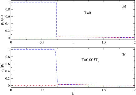
Figure 3: The momentum space density profile for mass symmetric case $q=1$ at (a) $T=0$ (b) $T=0.005T_{\rm F}.$ Here $(k_{F}a)^{-1}=2$ and $P=0.2.$ The profile corresponds to BP1 phase.

The figure 3 shows the density profile for mass symmetric case at zero and finite temperatures in the BEC regime of interaction. The density profile here corresponds to $(k_{F}a)^{-1}=2$ and $P=0.2$ and has the characteristic of BP1 phase of a single fermi surface. We also verify here that the thermodynamic potential difference between the paired phase and the normal matter is negative indicating its stability. The critical polarization $P_{c}$ up to which this phase is stable for this coupling is $P_{c}=0.52.$ As the coupling increases, the critical polarization $P_{c}$ increases and finally reaches $P_{c}=1$ at $(k_{f}a)^{-1}\approx 2.3$. The upper and lower curves correspond to zero temperature and $T/T_{F}=0.005$. Finite temperature effects smoothen the distribution functions.

We also observe that, at unitarity ($(k_{f}a)^{-1}$=0), breached pair solution exists with two fermi surfaces (BP2). However it is thermodynamically unstable i.e. $\delta\Omega$ is positive. The density profile in momentum space is shown in the Fig. 4. We have also shown the effect of temperature in the density profiles within the present mean field calculation. As before, the density profiles get smoothened for finite temperatures as quasi-particle density distribution is no longer a $\Theta(\ldots)$ function.

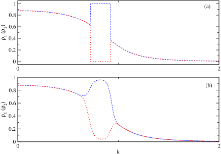
Figure 4: The momentum space density profile for mass symmetric case $q=1$ at (a) $T=0$ (b) $T=0.005T_{\rm F}.$ Here $(k_{F}a)^{-1}=0$ and $P=0.2.$ The profile corresponds to BP2 phase. This phase, however, is unstable.

We next consider the mass asymmetric case with the mass ratio $q=m_{1}/m_{2}$ differing from unity. Specifically, we have taken the mass ratio $q=0.15$. This ratio corresponds to ⁶Li-⁴⁰K mixture, which has been cooled to degeneracy recently taglieber , with ⁶Li chosen as the majority population. The momentum space density profile for this system at $(k_{F}a)^{-1}=0.1$ and $P=0.2.$ is shown in the Fig. 6. Though the coupling strength is close to unitarity, the phase corresponds to the gapless modes with one fermi surface (BP1). The critical polarization turns out to be $P_{c}\approx 0.35.$

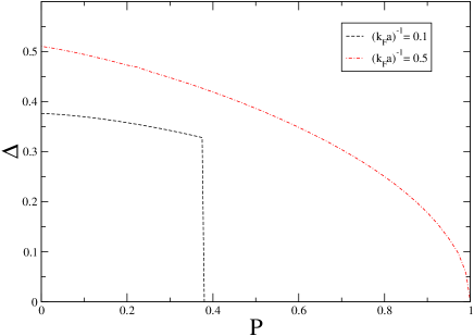
Figure 5: The variation of $\Delta$ against polarization is shown for $m_{1}/m_{2}=0.15$ at couplings $(k_{F}a)^{-1}=0.1$ (dashed) and $(k_{F}a)^{-1}=0.5$ (dot-dashed).

We see the breached pairing solution here with one fermi surface in the deep BEC regime. For example for $(k_{F}a)^{-1}=8$, we find the stable BP1 state up to the critical polarization $P_{c}\approx 0.22.$

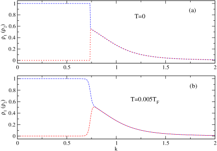
Figure 6: The momentum space density profile for mass asymmetric case $q=0.15$ at (a) $T=0$ (b) $T=0.005T_{\rm F}.$ Here $q=m_{1}/m_{2}$, $(k_{F}a)^{-1}=0.1$ and $P=0.2.$ The profile corresponds to BP2 phase. This is stable phase.

V summary and conclusions

We have considered here a variational ground state for the system of nonrelativistic fermions with a four fermion point interaction to model the phase structure of the cold atomic mixture near the Feshbach resonance. The ansatz functions including the thermal distribution functions describing the variational ground state are determined through the minimization of the thermodynamic potential. The stability of the solutions is decided by comparing the thermodynamic potentials of the paired state and normal matter.

We find that gapless modes with a single fermi surface solutions are possible within in the BEC region of the coupling constant when there is a difference of number densities of the two species. We have in particular looked into the number density difference of the two species differing in their masses. There is a critical polarization for a given coupling which can sustain pairing. Beyond this value for polarization the pairing state becomes unstable. We have not calculated the Meissner masses kitazawa or the number susceptibility gubankova to discuss the stability of different phases. Instead, we have solved the gap equations and the number density equations self consistently and have compared the thermodynamic potentials. In certain regions of couplings, we have multiple solutions of the gap equations. In such cases we have chosen the one which has the least value for the thermodynamic potential.

The present results however are limited by the simplified ansatz as considered here in terms of fermion condensates. To look into the thermal effects we have considered rather small temperatures. At higher temperature, particularly near the critical temperature, the effects of fluctuations involving corrections arising from collective modes will play an important role, particularly for strong coupling. Further, considering a realistic potential rather than the point interaction as considered here as well as the calculation of some of the transport properties in the different phases of cold atomic gas, will be very interesting to investigate and can be studied within the present framework. Some of these calculations are in progress and will be reported elsewhere.

- (1) B. DeMarco and D. S. Jin, Science 285, 1703 (1999); A. G. Truscott et al., Science 291, 2570 (2001)
- (2) C.A. Regal, M. Greiner and D.S. Jin, Phys. Rev. Lett. 92, 040403 (2004); M. Bartenstein et al, Phys. Rev. Lett. 92, 120401 (2004); M. W. Zwierlein et al, Phys. Rev. Lett. 92, 120403 (2004); J. Kianast et al, Phys. Rev. Lett. 92, 150402 (2004); T. Bourdel et al, Phys. Rev. Lett. 93, 050401 (2005).
- (3) C. Chin, M. Bartenstein, A. Altmeyer, S. Riedl, S. Jochim, J. Hecker Denschlag, and R. Grimm, Science 305, 1128 (2004)
- (4) M. W. Zwierlein, J. R. Abo-Shaeer, A. Schirotzek, C. H. Schunk, and W. Ketterle, Nature 435, 1047 (2005).
- (5) e.g. see review R. Casalbuoni and G. Nardulli, Rev. Mod. Phys. 76, 263 (2004)
- (6) A. Sedrakian, J. Mur-Petit, A. Polls, and Muther, arXiv:cond-mat/0404577v2; A. Sedrakian, J. Mur-Petit, A. Polls, and Muther, Phys. Rev. A 72, 013613 (2005).
- (7) P. F. Bedaque, H. Caldas, and G. Rupak, Phys. Rev. Lett. 91, 247002 (2003); Heron Caldas,Phys. Rev. A 69, 063602 (2004).
- (8) W.V. Liu and F. Wilczek,Phys. Rev. Lett. 90, 047002 (2003),E. Gubankova, W.V. Liu and F. Wilczek, Phys. Rev. Lett. 91, 032001 (2003).
- (9) Shin-Tza Wu and C.-H. Pao, Phys. Rev. B 74, 224504 (2006)
- (10) D. E. Sheehy and L. Radzihovsky, Phys. Rev. Lett. 96, 060401 (2006)
- (11) M. M. Parish, F. M. Marchetti, A. Lamacraft, and B. D. Simons, Nature Phys. 3, 124 (2007).
- (12) Shin-Tza Wu, C.-H. Pao, and S.-K. Yip Phys. Rev. B 74, 224504 (2006)
- (13) M. M. Parish, F. M. Marchetti, A. Lamacraft, and B. D. Simons, Phys. Rev. Lett. 98, 160402 (2007)
- (14) M.W. Zweierlein, A. Schirotzek, C.H. Schunck and W. Ketterle, Science,311,492 (2006); G.B. Patridge, W. Li, R.I Kamar, Y. Liao and R.G. Hulet, Science, 311, 503 (2006).
- (15) M. Taglieber, A.-C. Voigt, T. Aoki, T.W. Hänsch, and K. Dieckmann, Phys. Rev. Lett. 100, 010401 (2008).
- (16) E. Wille et al., Phys. Rev. Lett. 100, 053201 (2008).
- (17) C.A.R. Sa de Melo, M. Randeria and J.R. Engelbrecht, Phys. Rev. Lett. 71, 3202 (1993).
- (18) B. Deb, A.Mishra, H. Mishra and P. Panigrahi, Phys. Rev. A 70,011604(R), 2004.
- (19) A. Mishra and H. Mishra, arXiv:cond-mat/0611058.
- (20) Amruta Mishra and Hiranmaya Mishra, Phys. Rev. D 69, 014014 (2004); Phys. Rev. D 71, 074023 (2005); Phys. Rev. D 74, 054024 (2006)
- (21) H. Umezawa, H. Matsumoto and M. Tachiki Thermofield dynamics and condensed states (North Holland, Amsterdam, 1982) ; P.A. Henning, Phys. Rep.253, 235 (1995).
- (22) H. T. C. Stoof, M. Houbiers, C. A. Sackett, and R. G. Hulet, Phys. Rev. Lett. 76, 10 - 13 (1996)
- (23) M. Kitazawa, D. Rischke and I. Shovkovy, Phys Lett B637, 367, 2006.
- (24) E. Gubankova, A. Schmitt, F. Wilczek, Phys. Rev. B74, 064505 (2006).