Serially-regulated biological networks fully realize a constrained set of functions

Abstract

We show that biological networks with serial regulation (each node regulated by at most one other node) are constrained to direct functionality, in which the sign of the effect of an environmental input on a target species depends only on the direct path from the input to the target, even when there is a feedback loop allowing for multiple interaction pathways. Using a stochastic model for a set of small transcriptional regulatory networks that have been studied experimentally Guet et al. (2002), we further find that all networks can achieve all functions permitted by this constraint under reasonable settings of biochemical parameters. This underscores the functional versatility of the networks.

A driving question in systems biology in recent years has been the extent to which the topology of a biological network determines or constrains its function. Early works have suggested that the function follows the topology Shen-Orr et al. (2002); Mangan and Alon (2003); Guet et al. (2002); Kollmann et al. (2005), and this continues as a prevailing view even though later analyses (at least in a small corner of biology) have questioned the paradigm Wall et al. (2005); Ziv et al. (2007). It remains unknown if a small biochemical or regulatory network can perform multiple functions, and whether the function set is limited by the network’s topological structure. To this extent, in this paper, we develop a mathematical description of the functionality of a certain type of biological network, and show that the answer to both questions is “yes”: the networks can perform many, but not all possible functions, and the set of attainable functions is constrained by the topology. We illustrate these results in the context of an experimentally realized system Guet et al. (2002).

Following Guet et al. (2002) and our earlier work Ziv et al. (2007), we focus on the steady-state functionality of transcriptional regulatory networks. In this case, the input is the “chemical environment,” that is a binary vector of presence/absence of small molecules that affect the regulation abilities of the transcription factors; and the output is the steady-state expression of a particular gene, hereafter called the reporter. Different functions of the network correspond then to different ways to map the small molecule concentrations into the reporter expression.

In our setup, the effect of introducing a small molecule S_j specific to a transcription factor X_j is to modify the affinity of X_j to its binding site. Equivalently one can think of S_j as modulating or renormalizing the transcription factor concentration $X_{j}$ by some factor $s_{j}$, making the effective concentration $\chi_{j}=\chi_{j}(X_{j},s_{j})$. A simple example of such a modulation function is

$$\chi_{j}(X_{j},s_{j})\equiv X_{j}/s_{j},$$ (1)

in which the presence of the small molecule reduces the effective concentration of transcription factor by the factor $s_{j}$.

The function of the circuit will depend on how the steady-state expression $G^{*}$ of the reporter gene G changes as the modulation factor $s_{j}$ is varied from some “off” value $s_{j}^{-}$ to some “on” value $s_{j}^{+}$:

$$\frac{\Delta G^{*}}{\Delta s_{j}}=\frac{G^{*}(s_{j}^{+})-G^{*}(s_{j}^{-})}{\Delta s_{j}}=\frac{1}{\Delta s_{j}}\int_{s_{j}^{-}}^{s_{j}^{+}}\frac{dG^{*}}{ds_{j}}\,ds_{j},$$ (2)

where $\Delta s_{j}=s_{j}^{+}-s_{j}^{-}$. For example, if $\chi_{j}=X_{j}/s_{j}$, then $s_{j}^{-}=1$, indicating that the small molecule is absent, and $s_{j}^{+}>1$ is the factor by which effective concentration is reduced when the small molecule is present.

If the sign of $dG^{*}/ds_{j}$ does not change for $s_{j}\in[s_{j}^{-},s_{j}^{+}]$, then the sign of $\Delta G^{*}$ is fixed. For networks with only serial regulation, i.e. each gene is regulated by at most one other gene, we will show that the sign of $dG^{*}/ds_{j}$ is unique and in accord with the direct path from S_j to G, a property we term direct functionality. This constrains the possible responses and hence the functionality of serial networks. Importantly, we will then show that all admissible functions indeed can be attained by all the networks we studied operating at different parameter values. While throughout this work we focus on the setup pioneered experimentally by Guet et al. Guet et al. (2002), we also show that the constraint to direct functionality holds for any network with serial regulation.

I Direct functionality in small networks

As in Guet et al. Guet et al. (2002), we consider networks with $N$ = 4 genes (three transcription factors plus a reporter G), in which each gene is regulated by exactly one other gene. This admits three topologies and a total of 24 networks, as described in Fig. 1. All three topologies consist of a cycle and a cascade that begins in the cycle and ends at the reporter gene G. Once outside the cycle, there is only one path to G, so it suffices to study a topology consisting of an $n$-gene cycle with a gene G immediately outside (Fig. 1c is an example with $n=3$), and extensions to topologies where the cycle is connected to the reporter by a linear cascade are trivial.

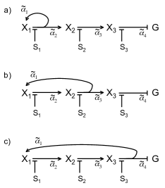
Figure 1: Four-gene networks (3 transcription factors X_i plus 1 reporter gene G) in which each gene is regulated by one other gene, as studied in Guet et al. (2002); Ziv et al. (2007). Transcription factor efficacies are influenced by small molecules S_i. Regulation functions $\tilde{\alpha}_{i}$ are assigned to the edges. The three edges $\tilde{\alpha}_{1}$, $\tilde{\alpha}_{2}$, and $\tilde{\alpha}_{3}$ can be up-regulating or down-regulating, giving $3\times 2^{3}=24$ possibilities; the reporter gene is repressed in all cases.

In this section, we will perform the steady-state analysis of such single-cycle networks to lay the groundwork for understanding the effect of topology on allowed functionality.

The process of protein expression has been modeled with remarkable success by combining transcription and translation into one step and directly coupling genes by a deterministic dynamics Elowitz and Leibler (2000); Gardner et al. (2000); Hasty et al. (2001). Accordingly we model mean expressions $\bar{X}_{i}$ (we later distinguish between entire probability distributions $P(X_{i})$ and the means of these distributions $\bar{X}_{i}$; cf. Appendix) with the system of ordinary differential equations

$$\frac{d\bar{X}_{1}}{dt} = \tilde{\alpha}_{1}(\bar{\chi}_{n})-r_{1}\bar{X}_{1},$$ (3)

$$\frac{d\bar{X}_{i}}{dt} = \tilde{\alpha}_{i}(\bar{\chi}_{i-1})-r_{i}\bar{X}_{i}\quad(2\leq i\leq n),$$ (4)

$$\frac{d\bar{G}}{dt} = \tilde{\alpha}_{n+1}(\bar{\chi}_{n})-r_{n+1}\bar{G},$$ (5)

where the $\tilde{\alpha}_{i}$ are creation rates for the species X_i (and $X_{n+1}\equiv G$), each monotonically regulated by the effective concentration $\bar{\chi}_{\pi_{i}}$ of its parent $\pi_{i}$, and the $r_{i}$ are the decay rates. Note that we have set

$$\pi_{1} = n,$$ (6)

$$\pi_{i} = i-1\quad(2\leq i\leq n+1)$$ (7)

to create the $n$-gene cycle with one gene immediately outside. The regulation functions $\tilde{\alpha}_{i}$ will be up- or down-regulating according to the network topology. A common example is the familiar Hill functions,

$$\tilde{\alpha}(\bar{\chi}) = a_{0}+a\frac{\bar{\chi}^{h}}{K^{h}+\bar{\chi}^{h}}\quad\textrm{(up-regulating)},$$ (8)

$$\tilde{\alpha}(\bar{\chi}) = a_{0}+a\frac{K^{h}}{K^{h}+\bar{\chi}^{h}}\quad\textrm{(down-regulating)},$$ (9)

with basal and maximal expression levels $a_{0}$ and $a_{0}+a$ respectively, Michaelis-Menten constants $K$, and cooperativities $h$. Although we use the functional forms in Eqns. (8-9), as well as the functional form for the modulation function in Eqn. (1), for our numerical experiment (cf. Numerical Results), the analytic result derived in this section will be valid for any monotonic functions $\tilde{\alpha}(\bar{\chi})$ and any function $\bar{\chi}(\bar{X},s)$.

Fixed points of the dynamical system in Eqns. (3-5) satisfy

$$\bar{X}_{1}^{*} = \alpha_{1}(\bar{\chi}_{n}^{*}),$$ (10)

$$\bar{X}_{i}^{*} = \alpha_{i}(\bar{\chi}_{i-1}^{*})\quad(2\leq i\leq n),$$ (11)

$$\bar{G}^{*} = \alpha_{n+1}(\bar{\chi}_{n}^{*}),$$ (12)

where we define

$$\alpha_{i}\equiv\tilde{\alpha}_{i}/r_{i}.$$ (13)

We may now, as in Kholodenko et al. (1997, 2002), use the chain rule to calculate the derivative of $\bar{G}^{*}$ with respect to a particular input factor $s_{j}$. For illustration, we will do so first for the concrete example in Fig. 1c, in which $n=3$. Let us consider the derivative of $\bar{G}^{*}$ with respect to $s_{1}$:

$$\frac{d\bar{G}^{*}}{ds_{1}}=\frac{\partial\alpha_{4}}{\partial\bar{X}_{3}}\frac{\partial\alpha_{3}}{\partial\bar{X}_{2}}\left[\frac{\partial\alpha_{2}}{\partial s_{1}}+\frac{\partial\alpha_{2}}{\partial\bar{X}_{1}}\frac{d\bar{X}_{1}^{*}}{ds_{1}}\right],$$ (14)

where all derivatives are evaluated at the fixed point, and it is understood that $\alpha_{i}$ depends on either $\bar{X}_{\pi_{i}}$ or $s_{\pi_{i}}$ through $\bar{\chi}_{\pi_{i}}$, that is, that

$$\frac{\partial\alpha_{i}}{\partial\bar{X}_{\pi_{i}}}=\frac{\partial\alpha_{i}}{\partial\bar{\chi}_{\pi_{i}}}\frac{\partial\bar{\chi}_{\pi_{i}}}{\partial\bar{X}_{\pi_{i}}}\quad{\rm and}\quad\frac{\partial\alpha_{i}}{\partial s_{\pi_{i}}}=\frac{\partial\alpha_{i}}{\partial\bar{\chi}_{\pi_{i}}}\frac{\partial\bar{\chi}_{\pi_{i}}}{\partial s_{\pi_{i}}}.$$ (15)

If we introduce the notation

$$\alpha_{i}^{\prime} \equiv \partial\alpha_{i}/\partial\bar{X}_{\pi_{i}},$$ (16)

$$\dot{\alpha_{i}} \equiv \partial\alpha_{i}/\partial s_{\pi_{i}},$$ (17)

then Eqn. (14) becomes

$$\frac{d\bar{G}^{*}}{ds_{1}}=\alpha^{\prime}_{4}\alpha^{\prime}_{3}\left[\dot{\alpha}_{2}+\alpha^{\prime}_{2}\frac{d\bar{X}_{1}^{*}}{ds_{1}}\right].$$ (18)

The first term reflects the direct chain to G from S₁, and the second term incorporates further contributions around the cycle and will need to be evaluated self-consistently.

For a cycle of arbitrary length $n$ and for an arbitrary input factor $s_{j}$ ($1\leq j\leq n$), Eqn. (18) generalizes to

$$\frac{d\bar{G}^{*}}{ds_{j}}=\left[\dot{\alpha}_{j+1}+\alpha^{\prime}_{j+1}\frac{d\bar{X}_{j}^{*}}{ds_{j}}\right]\prod_{k=j+2}^{n+1}\alpha^{\prime}_{k},$$ (19)

where we use the convention that

$$\prod_{k=a}^{b}[\cdot]=1\quad{\rm if}\quad a>b.$$ (20)

We may also use the chain rule for $d\bar{X}_{j}^{*}/ds_{j}$,

$$\frac{d\bar{X}_{j}^{*}}{ds_{j}} = \left[\dot{\alpha}_{(j\,{\rm mod}\,n)+1}+\alpha^{\prime}_{(j\,{\rm mod}\,n)+1}\frac{d\bar{X}_{j}^{*}}{ds_{j}}\right]$$ (21)

$$\times\frac{\prod_{k=1}^{n}\alpha^{\prime}_{k}}{\alpha^{\prime}_{(j\,{\rm mod}\,n)+1}}$$

and now we may solve for $d\bar{X}_{j}^{*}/ds_{j}$ self consistently:

$$\frac{d\bar{X}_{j}^{*}}{ds_{j}}=\frac{\dot{\alpha}_{(j\,{\rm mod}\,n)+1}}{\alpha^{\prime}_{(j\,{\rm mod}\,n)+1}}\frac{\prod_{k=1}^{n}\alpha^{\prime}_{k}}{1-\prod_{l=1}^{n}\alpha^{\prime}_{l}}.$$ (22)

For the special case of $j=n$, where $(j\,{\rm mod}\,n)+1=1$, substituting Eqn. (22) into Eqn. (19) obtains

$$\frac{d\bar{G}^{*}}{ds_{n}} = \left[\frac{1}{1-\prod_{l=1}^{n}\alpha^{\prime}_{l}}\right]$$ (23)

$$\times\left[\dot{\alpha}_{n+1}+(\dot{\alpha}_{1}\alpha^{\prime}_{n+1}-\dot{\alpha}_{n+1}\alpha^{\prime}_{1})\prod_{k=2}^{n}\alpha^{\prime}_{k}\right]$$

$$= \left[\frac{1}{1-\prod_{l=1}^{n}\alpha^{\prime}_{l}}\right]\dot{\alpha}_{n+1},$$ (24)

where the second step follows from

$$\dot{\alpha}_{1}\alpha^{\prime}_{n+1} = \left(\frac{d\alpha_{1}}{d\bar{\chi}_{n}}\frac{\partial\bar{\chi}_{n}}{\partial s_{n}}\right)\left(\frac{d\alpha_{n+1}}{d\bar{\chi}_{n}}\frac{\partial\bar{\chi}_{n}}{\partial\bar{X}_{n}}\right)$$ (25)

$$= \left(\frac{d\alpha_{1}}{d\bar{\chi}_{n}}\frac{\partial\bar{\chi}_{n}}{\partial\bar{X}_{n}}\right)\left(\frac{d\alpha_{n+1}}{d\bar{\chi}_{n}}\frac{\partial\bar{\chi}_{n}}{\partial s_{n}}\right)$$ (26)

$$= \alpha^{\prime}_{1}\dot{\alpha}_{n+1},$$ (27)

in which the first step recalls Eqn. (15). For $1\leq j\leq n-1$, where $(j\,{\rm mod}\,n)+1=j+1$, substituting Eqn. (22) into Eqn. (19) obtains

$$\frac{d\bar{G}^{*}}{ds_{j}}=\left[\frac{1}{1-\prod_{l=1}^{n}\alpha^{\prime}_{l}}\right]\dot{\alpha}_{j+1}\prod_{k=j+2}^{n+1}\alpha^{\prime}_{k},$$ (28)

which, upon inspection of Eqn. (24), is valid for $j=n$ as well.

Stability of the fixed point $\bar{X}^{*}_{j}$ requires that the Jacobian of Eqns. (3-4),

$$J=\left[\begin{array}[]{cccccc}-r_{1}&&&&&\tilde{\alpha}^{\prime}_{1}\\ \tilde{\alpha}^{\prime}_{2}&-r_{2}&&&&\\ &\tilde{\alpha}^{\prime}_{3}&-r_{3}&&&\\ &&\ddots&\ddots&&\\ &&&\tilde{\alpha}^{\prime}_{n-1}&-r_{n-1}&\\ &&&&\tilde{\alpha}^{\prime}_{n}&-r_{n}\\ \end{array}\right],$$ (29)

be negative definite or, since the determinant is the product of the eigenvalues, that

$$0 < (-1)^{n}\det(J)$$ (32)

$$=\prod_{k=1}^{n}r_{k}-\prod_{l=1}^{n}\tilde{\alpha}^{\prime}_{l}$$

$$=\prod_{k=1}^{n}r_{k}\left(1-\prod_{l=1}^{n}\alpha^{\prime}_{l}\right).$$

Since the decay rates $r_{k}$ are positive, Eqn. (32) says that the term inside the brackets in Eqn. (28) is positive for stable fixed points.

For the networks in Fig. 1, where in the 1- and 2-cycles the reporter is attached by means of intermediates, the analog of Eqn. (28) is calculated similarly to be

$$\frac{d\bar{G}^{*}}{ds_{j}}=\left[\frac{1}{1-\theta(n-j)\prod_{l=1}^{n}\alpha^{\prime}_{l}}\right]\dot{\alpha}_{j+1}\prod_{k=j+2}^{N}\alpha^{\prime}_{k},$$ (33)

where $N=4$ is the number of genes, $1\leq j\leq N-1$ for each of the 3 possible small molecule inputs, and $n$ is the length of the cycle ($1\leq n\leq N-1$). Here $\theta$ is the Heaviside function, for which we use the convention $\theta(0)=1$. Its presence reduces the bracketed term to 1 when the input S_j is outside the cycle, leaving only the contribution corresponding to the cascade from S_j to G, as must be the case.

In Eqn. (33), the term outside the brackets represents the direct (i.e., the shortest) path from S_j to G and fixes the sign of $d\bar{G}^{*}/ds_{j}$ (since the term inside the brackets is positive at a stable fixed point). If the creation rates are monotonic (which is the usual model for transcriptional regulation, but may be violated in protein signaling due to competitive inhibition and other effects), this sign is unique and fixes the sign of $\Delta\bar{G}^{*}/\Delta s_{j}$ via Eqn. (2). Importantly, this says that the feedback in each of the topologies in Fig. 1 is irrelevant in determining the sign of $\Delta\bar{G}^{*}/\Delta s_{j}$ for a steady-state analysis. As an example, for the network in Fig. 2a (inset), $\bar{G}^{*}$ changes with increasing $s_{1}$ according to $\dot{\alpha}_{2}\alpha^{\prime}_{3}\alpha^{\prime}_{4}$, which, since S₁ inhibits the activation, is negative $\times$ positive $\times$ negative $=$ positive, just as one would expect if the feedback was ignored.

I.1 Direct functionality corresponds to specific orderings of output states

Consider the case in which there are only two small molecule inputs, S₁ and S₂, as in Fig. 2a (inset). Since each input can be absent or present, $S_{1},S_{2}\in\{-,+\}$, there are four chemical input states $c=S_{1}S_{2}\in\{--,-+,+-,++\}$. Direct functionality admits only two orderings of the four output states $\bar{G}^{*}_{c}$, and hence the functionality of the network is severely limited by its serial topology. To see this, note that for Fig. 2a (inset) we have

$$\Delta\bar{G}^{*}/\Delta s_{1}\geq 0 \Rightarrow \bar{G}^{*}_{+-}\geq\bar{G}^{*}_{--}\textrm{ and}$$ (34)

$$\bar{G}^{*}_{++}\geq\bar{G}^{*}_{-+};$$

$$\Delta\bar{G}^{*}/\Delta s_{2}\geq 0 \Rightarrow \bar{G}^{*}_{-+}\geq\bar{G}^{*}_{--}\textrm{ and}$$ (35)

$$\bar{G}^{*}_{++}\geq\bar{G}^{*}_{+-}.$$

These conditions permit only the following output orderings, irrespective of biochemical parameters:

$$\bar{G}^{*}_{--} \leq \bar{G}^{*}_{-+}\leq\bar{G}^{*}_{+-}\leq\bar{G}^{*}_{++}\textrm{ or}$$

$$\bar{G}^{*}_{--} \leq \bar{G}^{*}_{+-}\leq\bar{G}^{*}_{-+}\leq\bar{G}^{*}_{++}.$$ (36)

These two orderings nevertheless allow the realization of a significant subset of all possible logical functions that one can build with two binary inputs, depending on the distinguishability of the four output states, as described in the next section. Quantifying the distinguishability demands careful treatment of the noise with a stochastic equivalent of our deterministic dynamical system, as described in the Appendix.

II Numerical results

We numerically solved the system in Eqns. (3-5) [with stochastic effects given by Eqn. (61)] with many parameter settings for all 24 networks represented in Fig. 1. In addition to verifying the restriction to direct functionality, we find that all networks can achieve all possible direct functions, suggesting that the networks are still quite versatile within the functional constraint.

For all networks, we consider the case of two small molecule inputs S₁ and S₂, as in the experimental setup of Guet et al. Guet et al. (2002), and as shown for an example network in Fig. 2a (inset). We take $s_{j}$ to be a multiplicative factor by which the transcription factor concentration $\bar{X}_{j}$ is effectively scaled, i.e.

$$\bar{\chi}_{j}(\bar{X}_{j},s_{j})\equiv\bar{X}_{j}/s_{j}.$$ (37)

Then $s_{j}^{-}\equiv 1$ for the “off” settings, and the $s_{j}^{+}>1$ are free parameters for the “on” settings.

We model the regulation using the familiar Hill form (which is monotonic and thus satisfies the direct functionality conditions)

$$\tilde{\alpha}(\bar{\chi}) = a_{0}+a\frac{\bar{\chi}^{h}}{K^{h}+\bar{\chi}^{h}}\quad\textrm{(up-regulating)},$$ (38)

$$\tilde{\alpha}(\bar{\chi}) = a_{0}+a\frac{K^{h}}{K^{h}+\bar{\chi}^{h}}\quad\textrm{(down-regulating)},$$ (39)

with basal and maximal expression levels $a_{0}$ and $a_{0}+a$ respectively, Michaelis-Menten constants $K$, and cooperativities $h$. For the 4-gene networks in Fig. 1, with only two small molecule inputs S₁ and S₂, this gives 22 parameters in total (cf. Table 1).

Parameters	Range
decay rates, $r_{i}$	$10^{-4}-10^{-3}$
Michaelis-Menten constants, $K_{i}$	$10^{0}-10^{3}$
basal expression levels, $a_{0,i}$	$10^{-3}-10^{-2}$
expression level ranges, $a_{i}$	$10^{0}-10^{2}$
cooperativities, $h_{i}$	$10^{0}-10^{1}$
“on” input factors, $s_{j}^{+}$	$10^{2}-10^{3}$

Table 1: Parameters and ranges from which each is randomly drawn, with $1\leq i\leq 4$ for the four genes, and $1\leq j\leq 2$ for the two small molecule inputs. Ranges are representative of typical cell conditions Elowitz and Leibler (2000); Braun et al. (2005).

For a given parameter set, we numerically solve Eqns. (3-5) (using Matlab’s ode15s) for each input state $c\in\{--,-+,+-,++\}$ to find mean steady-state concentrations $\bar{G}^{*}_{c}$. We then solve Eqn. (61) to find fluctuations around these means, giving probability distributions $P(G^{*}|c)$ (cf. Appendix). The function is defined by the ranking of the conditional distributions $P(G^{*}|c)$. That is, if two distributions are distinguishable, then the one with the larger mean is ranked higher. We consider two distributions to be indistinguishable when their means are separated by less than the smaller of their standard deviations (alternative definitions do not change our results qualitatively), in which case they both take on the average of their two ranks. When there are only two distinguishable output states, this rank-based classification reduces to that defining the familiar binary logical functions AND, OR, XOR etc. (see, for example, Fig. 2b, (ii-v)). More generally, for one, two, three, and four distinguishable responses, there are 75 total rankings (as listed on the horizontal axis of Fig. 2a). However, only 12 of these satisfy the ordering constraints for each network analogous to those in Eqn. (36) and therefore correspond to direct functions (for the newtork in Fig. 2a these 12 are shown in green on the horizontal axis).

We ran 50,000 trials for each of the 24 networks, in which the parameters were randomly selected (using a distribution uniform in log-space) from the ranges in Table 1. We found the steady-state reporter expression distributions $P(G^{*}|c)$ and classified the responses by ranking. All 24 networks displayed only direct functions. However, every network was able to achieve all 12 of its direct functions with parameters selected via Table 1, meaning that the networks fully realized all the functionality allowed by the constraint. This suggests that the networks studied are both constrained and versatile, and that a cell may still use a serial network to perform multiple logical functions by varying biochemical parameters, despite the restriction to direct functionality. Fig. 2 shows a histogram of functions and an example of each type of direct function for a representative network.

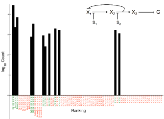
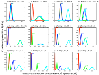
Figure 2: Direct functionality in a representative network with serial regulation (network shown in the inset in (a)). (a) Histogram of logical functions, as defined by the ranking of the output distributions $P(G^{*}|c)$ (cf. Numerical Results). Binary logic names are included after rankings when applicable, with ‘A’ and ‘B’ corresponding to inputs S₁ and S₂ respectively. Direct functions are labeled in green, indirect functions in red. Note that only direct functions are observed, and that all direct functions can be attained by the network. (b) An example of each direct function. Two distributions are considered indistinguishable in rank when their means are separated by less than the smaller of their standard deviations. For example, in (ix), the distributions for the first and second states ($--$ and $-+$ respectively) are indistinguishable, so they are tied in rank at 1.5 (the average of ranks 1 and 2). Note that all functions satisfy the ordering constraints in Eqn. (36).

We note that Guet et al. experimentally observed both direct and indirect functions Guet et al. (2002). However, they explicitly call the indirect functions into question, citing several possible unanticipated effects including RNA polymerase read-through. We have not incorporated such effects into the current model.

III Multiple fixed points

For the 12 networks in which the overall sign of the feedback cycle is positive, there are parameter settings that support multiple stable fixed points. In this section we evaluate the extent to which the presence of multiple fixed points affects the constraint to direct functionality, and we find that violation of the constraint is possible but unlikely.

While the function of a network has been defined in terms of $P(G^{*}|c)$, the linear noise approximation (cf. Appendix) only gives us access to $P(G^{*}|c,\bar{\bf X}^{*}_{m})$, the distribution expanded around a particular fixed point $\bar{\bf X}^{*}_{m}$. The two are related by a weighted sum,

$$P(G^{*}|c)=\sum_{m}\pi_{m}P(G^{*}|c,\bar{\bf X}^{*}_{m}),$$ (40)

where the probabilities $\pi_{m}$ of being near the $m$th fixed point will depend on the basins of attraction and curvatures near the fixed points. Numerical solution for $P(G^{*}|c)$ directly is possible in principle, although computationally difficult. Whether the statistical steady state distribution is calculated numerically or is approximated as in this manuscript, if we continue to define the function of the network by the ranking of the means of the $P(G^{*}|c)$, we have

$$\frac{d\bar{G}^{*}}{ds_{j}} = \frac{d}{ds_{j}}\int dG^{*}G^{*}P(G^{*}|c)$$ (41)

$$= \sum_{m}\frac{d}{ds_{j}}\pi_{m}\int dG^{*}G^{*}P(G^{*}|c,\bar{\bf X}^{*}_{m})$$ (42)

$$= \sum_{m}\left(\pi_{m}\frac{d\bar{G}^{*}_{m}}{ds_{j}}+\frac{d\pi_{m}}{ds_{j}}\bar{G}^{*}_{m}\right).$$ (43)

The expressions for the individual $d\bar{G}^{*}_{m}/ds_{j}$ are given by Eq. (33), so the first term in Eqn. (43) exhibits direct functionality. If the weights $\pi_{m}$ do not depend appreciably on the $s_{j}$, the second term will be small, and the restriction to direct functionality will be maintained. If, on the other hand, the weights do change appreciably (an obvious case might be the presence of a bifurcation at a particular value of $s_{j}$), then the second term may overpower the first enough to change the sign of $\Delta\bar{G}^{*}/\Delta s$ and violate the restriction to direct functionality.

We investigate this effect in two ways. First, we show analytically that, in the case of a 1-cycle, crossing a bifurcation does not violate direct functionality. Second, we subject all positive-feedback networks to a numerical test to estimate the dependence of the weights $\pi_{m}$ on the $s_{j}$. The results of both techniques suggest that the likelihood of a violation of direct functionality due to the presence of multiple fixed points is low.

III.1 Bifurcations do not violate direct functionality (1-D)

Consider the case of a positive 1-cycle with a gene G immediately outside, as shown in Fig. 3a (inset). For $n=1$, Eqns. (10-12) become

$$\bar{X}^{*} = \alpha_{1}(\bar{\chi}^{*}),$$ (44)

$$\bar{G}^{*} = \alpha_{2}(\bar{\chi}^{*}),$$ (45)

where unnecessary subscripts are dropped and $\bar{\chi}=\bar{X}/s$ as in Eqn. (37). With $\alpha_{1}$ of the form in Eqn. (38), there are at most two stable fixed points $\bar{X}_{1}^{*}$ and $\bar{X}_{2}^{*}$, with $\bar{X}_{1}^{*}<\bar{X}_{2}^{*}$, as illustrated by an example in Fig. 3a. As shown in Fig. 3b, bifurcations occur at $s_{1}$ and $s_{2}$ such that only $\bar{X}_{2}^{*}$ exists when $s<s_{1}$, only $\bar{X}_{1}^{*}$ exists when $s>s_{2}$, and $\bar{X}_{1}^{*}$ and $\bar{X}_{2}^{*}$ are found with (unknown) probabilities $\tilde{\pi}_{1}(s)$ and $\tilde{\pi}_{2}(s)=1-\tilde{\pi}_{1}(s)$ respectively when $s_{1}<s<s_{2}$. These statements can be combined such that

$$\pi_{1}(s)=\theta(s-s_{1})\theta(s_{2}-s)\tilde{\pi}_{1}(s)+\theta(s-s_{2})$$ (46)

and $\pi_{2}(s)=1-\pi_{1}(s)$ define the probabilities of approaching $\bar{X}_{1}^{*}$ and $\bar{X}_{2}^{*}$ respectively for any $s$. Here $\theta$ is the Heaviside function.

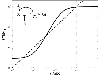
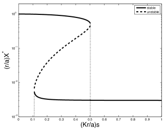
Figure 3: (a) Solid: plot of regulation function $\alpha_{1}=\tilde{\alpha}_{1}/r$ (refer to inset network), as defined in Eqns. (38) and (37), with parameters $h=2$, $a_{0}=0.03$, $a=10$, $K=2$, and $r=1$. Dashed line shows $\alpha_{1}=\bar{X}$ such that dotted lines indicate locations of stable fixed points $\bar{X}_{1}^{*}$ and $\bar{X}_{2}^{*}$ (take $\bar{X}_{2}^{*}>\bar{X}_{1}^{*}$). (b) Stable fixed points $\bar{X}_{m}^{*}$ (solid) and unstable fixed points (dashed) as a function of $s$, with $a_{0}/a=0.003$ as in (a). Dotted lines indicate locations of bifurcation points $s_{1}$ and $s_{2}$ such that only $\bar{X}_{2}^{*}$ exists when $s<s_{1}$, only $\bar{X}_{1}^{*}$ exists when $s>s_{2}$, and both $\bar{X}_{1}^{*}$ and $\bar{X}_{2}^{*}$ exist for $s_{1}<s<s_{2}$.

As we go from an “off” value $s^{-}$ to an “on” value $s^{+}$, let us assume that we hit both bifurcations, such that $s^{-}<s_{1}<s_{2}<s^{+}$. To test for direct functionality, we investigate the sign of

$$\frac{\Delta\bar{G}^{*}}{\Delta s} = \frac{1}{\Delta s}\int_{s^{-}}^{s^{+}}\sum_{m}\pi_{m}\frac{d\bar{G}^{*}_{m}}{ds}\,ds$$ (47)

$$+\frac{1}{\Delta s}\int_{s^{-}}^{s^{+}}\sum_{m}\frac{d\pi_{m}}{ds}\bar{G}^{*}_{m}\,ds$$

$$\equiv T_{1}+T_{2},$$ (48)

obtained using Eqns. (2) and (43). The first term $T_{1}$ depends on

$$\frac{d\bar{G}^{*}_{m}}{ds}=\frac{\dot{\alpha_{2}}}{1-\alpha^{\prime}_{1}}$$ (49)

(from Eqn. (28); $\alpha^{\prime}\equiv\partial\alpha/\partial\bar{X}$ and $\dot{\alpha}\equiv\partial\alpha/\partial s$ as before, both evaluated at the $m$th fixed point), which, as previously discussed, is always of the sign of $\dot{\alpha}_{2}$, consistent with direct functionality.

The second term $T_{2}$ can be written

$$T_{2} = \frac{1}{\Delta s}\int_{s^{-}}^{s^{+}}\left(\frac{d\pi_{1}}{ds}\bar{G}^{*}_{1}+\frac{d\pi_{2}}{ds}\bar{G}^{*}_{2}\right)\,ds$$ (50)

$$= \frac{1}{\Delta s}\int_{s^{-}}^{s^{+}}-\frac{d\pi_{1}}{ds}(\bar{G}^{*}_{2}-\bar{G}^{*}_{1})\,ds,$$ (51)

and since

$$\frac{d\pi_{1}}{ds} = \theta(s_{2}-s)\tilde{\pi}_{1}(s)\delta(s-s_{1})$$ (52)

$$+\left[1-\theta(s-s_{1})\tilde{\pi}_{1}(s)\right]\delta(s-s_{2})$$

$$+\theta(s-s_{1})\theta(s_{2}-s)\frac{d\tilde{\pi}_{1}}{ds},$$

(where $\delta$ is the Dirac delta function) we have

$$T_{2} = \frac{1}{\Delta s}\left\{-\left[\tilde{\pi}_{1}(\bar{G}^{*}_{2}-\bar{G}^{*}_{1})\right]_{s_{1}}-\left[\tilde{\pi}_{2}(\bar{G}^{*}_{2}-\bar{G}^{*}_{1})\right]_{s_{2}}\right.$$ (53)

$$\left.-\int_{s_{1}}^{s_{2}}\frac{d\tilde{\pi}_{1}}{ds}(\bar{G}^{*}_{2}-\bar{G}^{*}_{1})\,ds\right\}.$$

The first two terms in Eqn. (53) represent the contributions from crossing the bifurcations at $s_{1}$ and $s_{2}$ respectively. Using Eqn. (45) we may write them as

$$T_{2} = \frac{1}{\Delta s}\left\{\sum_{m=1}^{2}\left[\tilde{\pi}_{m}\left(-\frac{\Delta\alpha_{2}}{\Delta\bar{\chi}^{*}}\right)\Delta\bar{\chi}^{*}\right]_{s_{m}}\right.$$ (54)

$$\left.-\int_{s_{1}}^{s_{2}}\frac{d\tilde{\pi}_{1}}{ds}(\bar{G}^{*}_{2}-\bar{G}^{*}_{1})\,ds\right\},$$

where $\Delta\alpha_{2}=\alpha_{2}(\bar{\chi}_{2}^{*})-\alpha_{2}(\bar{\chi}_{1}^{*})$ and $\Delta\bar{\chi}^{*}=\bar{\chi}_{2}^{*}-\bar{\chi}_{1}^{*}=(\bar{X}_{2}^{*}-\bar{X}_{1}^{*})/s>0$. Since $\alpha_{2}$ is monotonic in $\bar{X}$, $-\Delta\alpha_{2}/\Delta\bar{\chi}^{*}$ at fixed $s$ is of the same sign as $-\alpha^{\prime}_{2}$, which is of the same sign as $\dot{\alpha}_{2}$ since $s$ effectively reduces $X$ (Eqn. (37)). Therefore the contributions to $\Delta\bar{G}^{*}/\Delta s$ from crossing the bifurcations do not violate direct functionality. A violation, at least in the case of a 1-cycle, can only come from variations in the probabilities $\tilde{\pi}_{m}$ within the region $s_{1}<s<s_{2}$, as described by the last term in Eqn. (54). Next we describe a numerical test that suggests such violations are rare.

III.2 Numerics suggest violations from multiple fixed points are rare

For each of the 12 positive-feedback networks, we numerically found the steady state of the dynamical system with randomly sampled parameters as before (cf. Numerical Results). However now for each parameter set we solved the system many times with randomly selected initial conditions. When multiple fixed points were found, the fraction of trials approaching the $m$th fixed point was used for the weight $\pi_{m}$. This assumes the $\pi_{m}$ are determined only by the basins of attraction of each fixed point, and by the distribution of the initial conditions. However, different distributions of initial conditions do not result in qualitative different results.

For each network, $2,000$ parameter sets were selected (uniform randomly in log-space), at which the system was solved $100$ times with initial protein counts selected uniform randomly from $0$ to $1,000$ proteins per cell. Over all positive-feedback networks, $37\%$ of the parameter sets supported multiple fixed points for at least one of the settings of S₁ and S₂. However only $0.46\%$ of parameter sets produced violations of direct functionality. Moreover this number is likely an overestimate, as no distinguishability criterion was imposed as was done in the single-fixed point case (cf. Numerical Results). It is likely that this fraction would remain low if the estimation of the $\pi_{m}$ was refined to incorporate the curvatures of the fixed points, or if alternative distributions were used for the sampling.

IV All networks with serial regulation exhibit only direct functionality

In this section, we extend our analytic constraint as derived in the context of the system studied experimentally by Guet et al. Guet et al. (2002) to show that any network with only serial regulation—each node having 0 or 1 parent—exhibits only direct functionality, i.e.  any target node X_i changes with any input S_j according to the direct path between them.

We first consider a connected directed graph in which every node has in-degree 1, called a contrafunctional graph Harary (1965). One can show that a contrafunctional graph has exactly one cycle, each of whose nodes is the root of a tree if the cycle edges are ignored Harary (1965). Now consider changing one node’s in-degree to 0, or equivalently, removing an edge. If the edge is in the cycle, the graph remains connected and becomes a tree. If the edge is not in the cycle, the graph is cut into two components: a contrafunctional graph and a tree.

A tree exhibits only direct functionality since there is at most one path from an input S_j to a gene X_i, which is therefore the direct path.

In a contrafunctional graph, we first consider the case where the target node X_i is inside the cycle. Only inputs S_j that are inside the cycle can affect X_i because the rest of the graph consists of trees that all point away from the cycle. Since we can start labeling nodes at any point in the cycle, we may take $i\leq j$ without loss of generality. Then, using the chain rule,

$$\frac{d\bar{X}_{i}^{*}}{ds_{j}} = \left[\dot{\alpha}_{(j\,{\rm mod}\,n)+1}+\alpha^{\prime}_{(j\,{\rm mod}\,n)+1}\frac{d\bar{X}_{j}^{*}}{ds_{j}}\right]$$ (56)

$$\times\frac{\prod_{k=1}^{n}\alpha^{\prime}_{k}}{\prod_{l=i}^{j}\alpha^{\prime}_{(l\,{\rm mod}\,n)+1}}$$

$$= \left[\frac{1}{1-\prod_{m=1}^{n}\alpha^{\prime}_{m}}\right]$$

$$\times\dot{\alpha}_{(j\,{\rm mod}\,n)+1}\frac{\prod_{k=1}^{n}\alpha^{\prime}_{k}}{\prod_{l=i}^{j}\alpha^{\prime}_{(l\,{\rm mod}\,n)+1}},$$

where the second step follows from Eqn. (22).

We next consider the case where the target node is outside the cycle. An input S_j can only affect the node if it is either in the cycle or above the node in its tree. The portion of the path in the tree will exhibit direct functionality. Therefore in looking for possible indirect functionality we may, without loss of generality, take the node to be immediately outside the cycle, as we did for G in the previous section. $d\bar{G}^{*}/ds_{j}$ is then given by Eqn. (28).

In both Eqns. (56) and (28), the term outside the brackets represents the direct path from S_j to the target node, and the term inside the brackets is positive for stable fixed points. Therefore, a contrafunctional graph exhibits only direct functionality. Since each connected component of a network in which every node has in-degree 0 or 1 is either a contrafunctional graph or a tree, such networks exhibit only direct functionality. Thus, in general, the possible logical functions of topologies with at most one regulator per node are severely constrained.

V Appendix: The stochastic model

The dynamical system in Eqns. (3-5) provides a deterministic description of mean expression levels but fails to capture fluctuations around these means. A full stochastic description is given by the chemical master equation. For $N$ species participating in $R$ elementary reactions in a system with volume $\Omega$, the master equation reads

$$\frac{dP({\bf n},t)}{dt}=\Omega\sum_{j=1}^{R}\left(\prod_{i=1}^{N}E^{-Z_{ij}}-1\right)f_{j}({\bf X},\Omega)P({\bf n},t),$$ (57)

where $P({\bf n},t)$ is the probability of having the copy number vector ${\bf n}=\Omega{\bf X}=\Omega(X_{1},\dots,X_{N})$ at time $t$, $Z_{ij}$ is the $N\times R$ stochiometric matrix, $E^{-Z_{ij}}$ is the step operator which acts by removing $Z_{ij}$ molecules from $n_{i}$, and $f_{j}$ is the rate for reaction $j$. The $f_{j}$ are the $\tilde{\alpha}_{j}$ and $r_{j}X_{j}$ of Eqns. (3-5) in the macroscopic limit.

As in previous work Ziv et al. (2007), we employ the much-used linear noise approximation Elf et al. (2003); Paulsson (2004); Elf and Ehrenberg (2003); van Kampen (1992) to make Eqn. (57) tractable by expanding in orders of $\Omega^{-1/2}$. Introducing ${\bf\xi}$ such that $n_{i}=\Omega X_{i}+\Omega^{1/2}\xi_{i}$ and treating ${\bf\xi}$ as continuous, the first two terms in the expansion yield the macroscopic rate equations (e.g. Eqns. (3-5) in our case) and the linear Fokker-Plank equation, respectively:

$$\sum_{i=1}^{N}\frac{\partial\bar{X}_{i}}{\partial t}\frac{\partial P({\bf\xi},t)}{\partial\xi_{i}}=\sum_{i=1}^{N}\sum_{j=1}^{R}Z_{ij}f_{j}({\bf\bar{X}})\frac{\partial P({\bf\xi},t)}{\partial\xi_{i}},$$ (58)

$$\frac{\partial P({\bf\xi},t)}{\partial t}=-\sum_{i,k}J_{ik}\frac{\partial(\xi_{k}P)}{\partial\xi_{i}}+\frac{1}{2}\sum_{i,k}D_{ik}\frac{\partial^{2}P}{\partial\xi_{i}\partial\xi_{k}},$$ (59)

where $J_{ik}=\sum_{j=1}^{R}Z_{ij}(\partial f_{j}/\partial X_{k})$ is the Jacobian matrix (e.g. Eqn. (29)) and $D_{ik}=\sum_{j=1}^{R}Z_{ij}Z_{kj}f_{j}({\bf X})$ is a diffusion-like matrix. The steady-state solution to Eqn. (59) is the multivariate Gaussian

$$P({\bf\xi})=\left[(2\pi)^{N}\det\Xi\right]^{-1/2}\exp\left(-\frac{-\xi^{T}\Xi\xi}{2}\right),$$ (60)

where the covariance matrix $\Xi$ satisfies

$$J\Xi+\Xi J^{T}+D=0.$$ (61)

We solve for $\Xi$ using standard matrix Lyapunov equation solvers (e.g., Matlab’s lyap). Thus fluctuations are captured to leading order by Gaussian distributions with means $\bar{X}_{i}$ given by the macroscopic equation and variances given by the diagonal entries of $\Xi$. For example, Gaussian distributions $P(G^{*}|c)$ are shown in Fig. 2b for the steady-state concentration of the reporter gene G under chemical input states $c$. In Ziv et al. (2007) we have compared the distributions $P(G^{*}|c)$ obtained using the linear noise approximation to those obtained via direct stochastic simulations Gillespie (1977) and found the results almost indistinguishable for molecular copy number above 10-20.

References

• Guet et al. (2002) C. C. Guet, M. B. Elowitz, W. Hsing, and S. Leibler, Science 296, 1466 (2002).
• Shen-Orr et al. (2002) S. S. Shen-Orr, R. Milo, S. Mangan, and U. Alon, Nat Genet 31, 64 (2002).
• Mangan and Alon (2003) S. Mangan and U. Alon, Proc Natl Acad Sci USA 100, 11980 (2003).
• Kollmann et al. (2005) M. Kollmann, L. Løvdok, K. Bartholomé, J. Timmer, and V. Sourjik, Nature 438, 504 (2005).
• Wall et al. (2005) M. E. Wall, M. J. Dunlop, and W. S. Hlavacek, J Mol Biol 349, 501 (2005).
• Ziv et al. (2007) E. Ziv, I. Nemenman, and C. H. Wiggins, PLoS ONE 2, e1077 (2007).
• Elowitz and Leibler (2000) M. B. Elowitz and S. Leibler, Nature 403, 335 (2000).
• Gardner et al. (2000) T. S. Gardner, C. R. Cantor, and J. J. Collins, Nature 403, 339 (2000).
• Hasty et al. (2001) J. Hasty, D. McMillen, F. Isaacs, and J. J. Collins, Nat Rev Genet 2, 268 (2001).
• Kholodenko et al. (1997) B. N. Kholodenko, J. B. Hoek, H. V. Westerhoff, and G. C. Brown, FEBS Lett 414, 430 (1997).
• Kholodenko et al. (2002) B. N. Kholodenko, A. Kiyatkin, F. J. Bruggeman, E. Sontag, H. V. Westerhoff, and J. B. Hoek, Proc Natl Acad Sci USA 99, 12841 (2002).
• Harary (1965) F. Harary, Structural models: an introduction to the theory of directed graphs (New York: John Wiley & Sons, 1965).
• Elf et al. (2003) J. Elf, J. Paulsson, O. G. Berg, and M. Ehrenberg, Biophys J 84, 154 (2003).
• Paulsson (2004) J. Paulsson, Nature 427, 415 (2004).
• Elf and Ehrenberg (2003) J. Elf and M. Ehrenberg, Genome Res 13, 2475 (2003).
• van Kampen (1992) N. G. van Kampen, Stochastic processes in physics and chemistry (Amsterdam: North-Holland, 1992).
• Gillespie (1977) D. T. Gillespie, J Phys Chem 81, 2340 (1977).
• Braun et al. (2005) D. Braun, S. Basu, and R. Weiss (2005), URL http://www.princeton.edu/~rweiss/papers/braun-2005.pdf.