One-dimensional anyons with competing $\delta$-function and derivative $\delta$-function potentials

Abstract

We propose an exactly solvable model of one-dimensional anyons with competing $\delta$-function and derivative $\delta$-function interaction potentials. The Bethe ansatz equations are derived in terms of the $N$-particle sector for the quantum anyonic field model of the generalized derivative nonlinear Schrödinger equation. This more general anyon model exhibits richer physics than that of the recently studied one-dimensional model of $\delta$-function interacting anyons. We show that the anyonic signature is inextricably related to the velocities of the colliding particles and the pairwise dynamical interaction between particles.

, and

1 Introduction

Anyons – which interpolate between bosons and fermions – may exist in two dimensions (2D), obeying fractional statistics. Fractional statistics have recently been observed in experiments on the quasiparticle excitations of a 2D electron gas in the fractional quantum Hall (FQH) regime [1]. The anyonic quasiparticles have profound implications for topological quantum states of matter [2]. For example, non-Abelian topological order can be studied through manipulating FQH states in a 2D electron gas. As a consequence, the concept of anyons has become important in topological quantum computation [3, 4]. In one dimension (1D) anyons acquire a step-function-like phase when two identical particles exchange their positions. Different aspects of anyons in 1D have been considered [5, 6, 7]. Among these an anyonic extension [8] of the 1D integrable Bose gas with $\delta$-function interaction [9, 10] has attracted recent attention, including the basic construction of the anyon model [11, 12, 13]. Many new results have been obtained for this model, including the connection with Haldane [14] exclusion statistics [15, 16], correlation functions [12, 17, 18, 19], entanglement [20] and expanding anyonic fluids [21].

A key feature of 1D anyons is that they retain fractional statistics in quasi-momentum space and the anyonic signature of the exchange interaction – the topological anyonic interaction and dynamical interaction are inextricably related. 1D anyons show an intriguing sensitivity of the boundary condition of their wave function on the specific position of the particles [11, 12, 23]. Therefore the study of exactly solvable interacting anyons in 1D should give insight into understanding topological effects in many-body physics.

In this communication we propose a 1D model of anyons with $\delta$-function and derivative $\delta$-function interaction and solve the model by means of the co-ordinate Bethe ansatz. The model contains an additional independent interaction parameter so that in principle one can study anyonic signatures through tuning the interactions. For this more general model we show that the anyonic signature is inextricably related to the velocities of the colliding particles and the pairwise dynamical interaction between identical particles.

2 The model

We consider creation and annihilation operators $\Psi^{\dagger}(x)$ and $\Psi(x)$ at point $x$, which satisfy the anyonic commutation relations

$$\Psi(x)\Psi^{\dagger}(y) = {\mathrm{e}}^{-\rmi\kappa w(x,y)}\Psi^{\dagger}(y)\Psi(x)+\delta(x-y)$$

$$\Psi^{\dagger}(x)\Psi^{\dagger}(y) = {\mathrm{e}}^{\rmi\kappa w(x,y)}\Psi^{\dagger}(y)\Psi^{\dagger}(x)$$

$$\Psi(x)\Psi(y) = {\mathrm{e}}^{\rmi\kappa w(x,y)}\Psi(y)\Psi(x).$$ (1)

The multi-step function $w(x,y)$ appearing in the phase factors satisfies $w(x,y)=-w(y,x)=1$ for $x>y$, with $w(x,x)=0$. In terms of these operators the hamiltonian describing $N$ anyons of atomic mass $m$ confined in a length $L$ is

$$H = \frac{\hbar^{2}}{2m}\int_{0}^{L}\rmd x\,\Psi^{\dagger}_{x}(x)\Psi_{x}(x)+\frac{1}{2}\,g\int_{0}^{L}\rmd x\,\Psi^{\dagger}(x)\Psi^{\dagger}(x)\Psi(x)\Psi(x)$$ (2)

$$+\rmi\epsilon\int_{0}^{L}\rmd x\,[\Psi^{\dagger}(x)\Psi^{\dagger}(x)\Psi(x)\Psi_{x}(x)-\Psi_{x}^{\dagger}(x)\Psi^{\dagger}(x)\Psi(x)\Psi(x)]$$

where we also impose periodic boundary conditions.

The tunable parameters in the model are (i) $g={\hbar^{2}c}/{m}$, the dynamical interaction strength which drives the particles in elastic scattering through zero range contact interaction, where $c$ is the coupling constant, (ii) the nonlinear dispersion coupling constant $\epsilon$, which describes a delta shift in collisions, and (iii) the statistical parameter $\kappa$ which varies the statistics of the particles from pure Bose statistics ($\kappa=0$) to pure Fermi statistics ($\kappa=\pi$). The model differs from the interacting 1D Bose gas [9, 10] and 1D interacting anyons [8] due to the presence of the nonlinear dispersion $\epsilon$, i.e., the s-wave scattering is disturbed by a delta shift in collisions. Effectively, the 1D scattering length is increased or decreased in individual pairwise collisions by this dispersion. It follows that the model contains well known models as special cases in certain limits. For $\kappa=0$, hamiltonian (2) reduces to that of the generalized nonlinear Schrödinger model [24, 26, 27], which has been studied by means of scattering Bethe ansatz in the context of soliton physics. For $\epsilon=0$, it describes the model of 1D interacting anyons. For $\kappa=\epsilon=0$, it reduces to the model of 1D interacting bosons, while for $\kappa=c=0$ it reduces to quantum derivative nonlinear Schrodinger model [28]. As we shall see, the general model (2) exhibits more exotic dynamics than the two models corresponding to the special cases $\kappa=0$ and $\epsilon=0$.

For convenience, we hereafter set $\hbar=2m=1$. We also use a dimensionless coupling constant $\gamma=c/n$ to characterize different physical regimes of the anyon gas, where $n=N/L$ is the linear density.

3 Bethe Ansatz

We first present the corresponding equation of motion $-\rmi\,\partial_{t}\Psi(x,t)=\left[H,\Psi(x,t)\right]$ via the time-dependent quantum fields, i.e., the nonlinear Schrödinger equation is given by

$$\rmi\Psi_{t}=-\Psi_{xx}+g\Psi^{\dagger}\Psi\Psi+4\rmi\epsilon\,\Psi^{\dagger}\Psi\Psi_{x}.$$ (3)

We note that this is an anyonic version of the generalized nonlinear Schrödinger equation. Restricting to its $N$-particle sector we can reduce the eigenvalue problem of the hamiltonian (2) to a quantum many-body problem. To this end, we define a Fock vacuum state $\Psi(x)|0\rangle=0$. Thus we can prove that the number operator $N$ and momentum operator $P$ are conserved, where

$$N = \int_{0}^{L}\rmd x\,\Psi^{\dagger}(x)\Psi(x)$$ (4)

$$P = \rmi\int_{0}^{L}\rmd x\,\Psi_{x}^{\dagger}\Psi(x).$$ (5)

In order to properly assign the anyonic phase $w(x_{i},x_{j})$ [8, 15, 11, 12] in the domain $x_{1}<x_{2}<\ldots<x_{N}$, we write the $N$-particle eigenstate as

$$\mid\!\Phi\rangle=\int_{0}^{L}\rmd x^{N}{\rme}^{-\rmi\frac{1}{2}{\kappa N}}\chi(x_{1}\ldots x_{N})\Psi^{\dagger}(x_{1})\ldots\Psi^{\dagger}(x_{N})\!\mid\!0\rangle$$ (6)

where the wavefunction amplitude is of the form

$$\chi(x_{1}\ldots x_{N}) = {\rme}^{-\rmi\frac{1}{2}\kappa\sum_{x_{i}<x_{j}}^{N}w(x_{i},x_{j})}\sum_{P}A(k_{P1}\cdots k_{PN}){\rme}^{\rmi(k_{P1}x_{1}+\ldots+k_{PN}x_{N})}.$$ (7)

Here the sum extends over all $N!$ permutations $P$. The choice of the sign of the anyonic phase factor in equation (7) can be arbitrary and may lead to different boundary conditions [12]. Here we prefer to a fix a boundary condition where we count the anyonic phase factor in equation (7) through the order of the particles in the scattering states [11]. By acting on the eigenstate (6) with hamiltonian (2) the eigenvalue problem for hamiltonian (2), namely

$$H\mid\!\Phi\rangle=\int_{0}^{L}\rmd x^{N}{\mathrm{e}}^{-\rmi\frac{1}{2}{\kappa N}}H_{N}\chi(x_{1}\ldots x_{N})\Psi^{\dagger}(x_{1})\ldots\Psi^{\dagger}(x_{N})\!\mid\!0\rangle$$ (8)

can be reduced to solving the quantum mechanical problem

$$H_{N}\chi(x_{1}\ldots x_{N})=E\chi(x_{1}\ldots x_{N})$$ (9)

where

$$H_{N} = -\sum_{i=1}^{N}\frac{\partial^{2}}{\partial x_{i}^{2}}+g\sum_{1\leq i<j\leq N}\delta(x_{i}-x_{j})$$ (10)

$$+\,\rmi\,2\epsilon\sum_{1\leq i<j\leq N}\delta(x_{i}-x_{j})(\partial_{x_{i}}+\partial_{x_{j}}).$$

This anyon model turns out to be Bethe ansatz solvable with independent values of $c$, $\epsilon$ and $\kappa$. Changing the coordinates to centre of mass coordinates $X=({x_{j}+x_{k}})/{2}$ and $Y=x_{j}-x_{k}$ leads to the eigenvalue equation (9) in the form

$$\left\{\left(-\frac{\partial^{2}}{\partial x_{1}^{2}}\cdots-\frac{1}{2}\frac{\partial^{2}}{\partial X^{2}}-2\frac{\partial^{2}}{\partial Y^{2}}\cdots-\frac{\partial^{2}}{\partial x_{N}^{2}}\right)\right.$$

$$\left.\phantom{\frac{\partial^{2}}{\partial x_{1}^{2}}}+2c\delta(Y)+\rmi\,4\epsilon\delta(Y)\partial_{X}-E\right\}\chi(\ldots x_{i}\ldots x_{j}\ldots)=0.$$ (11)

Integrating both sides of this equation with respect to $Y$ from $-e$ to $+e$ and taking the limit ${e\to 0}$ gives the discontinuity condition

$$\left(\partial_{x_{j}}-\partial_{x_{i}}\right)\chi(x_{1},\ldots,x_{i},x_{j},\ldots,x_{N})|_{x_{j}=x_{i}+e}$$

$$-\left(\partial_{x_{j}}-\partial_{x_{i}}\right)\chi(x_{1},\ldots,x_{j},x_{i},\ldots,x_{N})|_{x_{j}=x_{i}-e}$$

$$=[2c+\rmi\,2\epsilon(\partial_{x_{i}}+\partial_{x_{j}})]\chi(x_{1},\ldots,x_{i},x_{j},\ldots,x_{N})|_{x_{i}=x_{j}}$$ (12)

on the derivative of the wavefunction. This equation gives a relation between the coefficients $A(k_{P1}\ldots k_{PN})$ of the form

$$A(\ldots k_{j},k_{i}\ldots)=\frac{k_{j}-k_{i}+\rmi(c^{\prime}-\epsilon^{\prime}(k_{j}+k_{i}))}{k_{j}-k_{i}-\rmi(c^{\prime}-\epsilon^{\prime}(k_{j}+k_{i}))}A(\ldots k_{i},k_{j}\ldots)$$ (13)

which is the two-body scattering relation. This relation gives rise to a functional scalar scattering matrix which factorizes three-body scattering processes into the product of three two-body scattering matrices [24]. In this sense the Yang-Baxter equation is trivially satisfied, guaranteeing no diffraction in the scattering process [10, 24]. Consequently the $N$-particle scattering amplitude can be factorized into the products of two-particle amplitudes. Another way to establish the integrability of the model is to explicitly construct an infinite number of higher order conserved quantities, as shown for the 1D Bose gas in Ref. [25].

The effective interaction strengths $c^{\prime}$ and $\epsilon^{\prime}$ appearing in the solution are given by

$$c^{\prime}=\frac{c}{\cos(\kappa/2)}\qquad{\rm and}\qquad\epsilon^{\prime}=\frac{\epsilon}{\cos(\kappa/2)}.$$ (14)

In this model these effective coupling constants implement the transmutation between statistical and dynamical interactions.

To complete the solution in terms of the Bethe ansatz we impose the periodic boundary condition $\chi(x_{1}=0,x_{2}\ldots,x_{N})=\chi(x_{2},\ldots,x_{N},x_{1}=L)$ on the anyonic wavefunction in the fundamental region $0\leq x_{1}<x_{2}<\ldots<x_{N}\leq L$. As in the solution of the interacting anyon model ($\epsilon=0$), this leads to the appearance of various phase factors [11, 12]. The wave functions for other regions can be determined through application of the anyonic symmetry. The periodic boundary condition can also be imposed on other wavefunction arguments $x_{i}$, in each case leading to the same anyonic phase factor in the Bethe ansatz equations (BAE) [11, 12]. For this model, the energy is given by

$$E=\sum_{i=1}^{N}k_{i}^{2}$$ (15)

where the quasi-momenta $k_{j}$ satisfy the BAE

$${\mathrm{e}}^{\rmi k_{j}L}=-{\mathrm{e}}^{\rmi\kappa(N-1)}\prod^{N}_{\ell=1}\frac{k_{j}-k_{\ell}+\rmi\,(c^{\prime}-\epsilon^{\prime}(k_{j}+k_{\ell}))}{k_{j}-k_{\ell}-\rmi\,(c^{\prime}-\epsilon^{\prime}(k_{j}+k_{\ell}))}$$ (16)

for $j=1,\ldots,N$. The total momentum is

$$p=\sum_{i=1}^{N}k_{i}=N(N-1)\kappa/L.$$ (17)

In minimizing the energy we consider $\kappa(N-1)=\nu$ (mod $2\pi$) in the phase factor.

The Bethe ansatz solution provides in principle the full physics of the model. For the case $\kappa=0$, the BAE (16) are consistent with the scattering states constructed for the generalized nonlinear Schrödinger model [24, 26]. It is also clear to see from the BAE (16) that the phase shift

$$\theta_{j,\ell}=\ln\left[\frac{k_{j}-k_{\ell}+\rmi\,(c^{\prime}-\epsilon^{\prime}(k_{j}+k_{\ell}))}{k_{j}-k_{\ell}-\rmi\,(c^{\prime}-\epsilon^{\prime}(k_{j}+k_{\ell}))}\right]$$ (18)

depends essentially on the anyon parameter $\kappa$, the dynamical interaction strength $c$ and the nonlinear dispersion of velocity $\epsilon$ through the effective interactions (14). Among the competing interactions, the nonlinearity parameter $\epsilon$ is essential in determining the bound states. The $\delta$-function interaction strength $c$ plays the role of a driving force in collisions. However, the anyonic parameter $\kappa$ determines the statistical signature of the particles.

4 Preliminary analysis

The asymptotic behaviour of the BAE (16) reveals that bound states exist for $c<0$ and $c<2\epsilon\nu/L$. In general, the form of the bound states appears to be extremely complicated. For example, for $N=2$ and $L(c-p\epsilon)\gg 1$, we have the bound state $\left\{\frac{1}{2}p\pm\rmi\frac{1}{2}(c-p\epsilon)\right\}$. In this communication we focus on the repulsive regime, where $c>0$ and $|\epsilon|<c/(2p)$, for which the Bethe roots are real.

In the weak coupling limit $\gamma\ll\cos(\kappa/2)$, the leading term for the ground state energy, obtained from the BAE (16), is

$$\frac{E_{0}}{N}\approx\frac{(N-1)}{L}\left(c^{\prime}-2\epsilon^{\prime}\nu/L\right)+\,\frac{\nu^{2}}{L^{2}}.$$ (19)

To this order, for $\kappa=0$ the ground state energy is independent of the nonlinear dispersion $\epsilon$ and reduces to that of weakly interacting bosons. However, the quasimomentum distribution

$$g((k_{j}+k_{j+1})/2)=\frac{1}{L(k_{j+1}-k_{j})}.$$ (20)

deviates from the usual semicircle law [9, 30, 31] at $\epsilon=0$ (see figure 1). For $\epsilon>0$, the high density distribution drifts to the right hand side and the front becomes steeper as the nonlinear dispersion $\epsilon$ increases. For $\epsilon<0$, the high density part drifts to the left hand side. The nature of this kind of quantum drift in quasimomentum space is due to the delta shift or equivalently the nonlinear dispersion of velocity, which effectively increases or decreases the 1D scattering length in individual pairwise collisions.

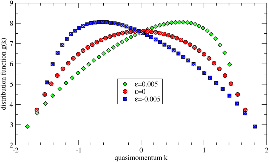
Figure 1: Typical figure showing the quantum drift effect of the nonlinear dispersion $\epsilon$ on the quasimomentum distribution function. Here $\kappa=0$, $c=0.04$, $L=2$ and $N=45$. Drifts to the left and right are symmetric with respect to the sign of $\epsilon$.

When the total momentum is non zero, i.e. $p\neq 0$, the left and right drifts are no longer symmetric with respect to the sign of $\epsilon$. Here the anyonic parameter $\kappa$ also introduces quantum drifts in quasimomentum space. A particular example is illustrated in figure 2. For $\epsilon>0$, the front of the distribution become very steep and the width becomes narrower as $\epsilon$ increases. The energy decreases as $\epsilon$ increases. However, for $\epsilon<0$, the distribution becomes flatter. In this case, the energy increases as $|\epsilon|$ increases.

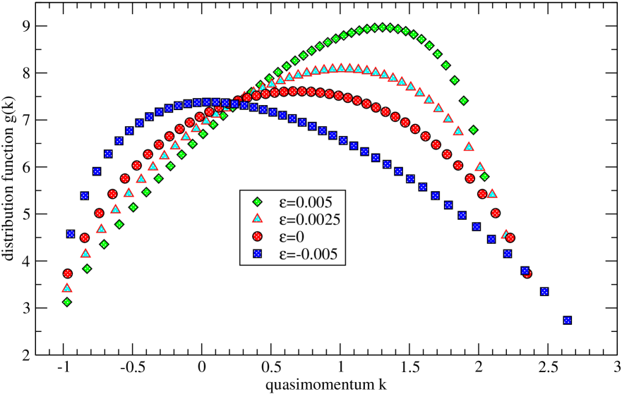
Figure 2: Typical figure showing the quantum drift effect in the quasimomentum distribution function with nonlinear dispersion $\epsilon$ and anyonic parameter $\kappa$. Here $\kappa={\pi}/{100}$, $c=0.04$, $L=2$ and $N=45$. The drifts is no longer symmetric with respect to the sign of $\epsilon$.

In the strong coupling limit $Lc\gg 1$, one can perform the strong coupling expansion with the BAE (16). In this limit the ground state of the model becomes that of the Tonks-Girardeau gas. This is mainly because in the strong repulsive limit, the particles behave like fermions in thermalized states. As a result the effect induced by the nonlinear dispersion of velocity is suppressed. To obtain the explicit result for the ground state energy, let all quasimomenta $k_{j}$ shift to $\lambda_{j}=k_{j}-\nu/L$ and for simplicity, choose $N$ to be odd. In this limit, the quasimomenta are given explicitly by

$$\lambda_{j} \approx \left[\frac{2n_{j}\pi}{L}\left(1-\frac{4n_{j}\epsilon^{\prime}\pi}{(Lc^{\prime}-\epsilon^{\prime}\nu)^{2}}\right)+\frac{2\epsilon^{\prime}N(N^{2}-1)\pi^{2}}{3L(Lc^{\prime}-\epsilon^{\prime}\nu)^{2}}\right]\left(1+\frac{2N}{(Lc^{\prime}-\epsilon^{\prime}\nu)}\right)^{-1}$$ (21)

where $n_{j}=-(N-1)/2,\ldots,(N-1)/2$. This result indicates that $\sum_{j=1}^{N}\lambda_{j}=0$. The corresponding ground state energy is given by

$$\frac{E_{0}}{N}\approx\frac{(N^{2}-1)\pi^{2}}{3L^{2}}\left(1+\frac{2N}{(Lc^{\prime}-\epsilon^{\prime}\nu)}\right)^{-2}+\,\frac{\nu^{2}}{L^{2}}.$$ (22)

It can be seen from the Bethe roots (21) that the flat fermion-like distribution becomes inclined as $|\epsilon|$ becomes large. The distribution almost linearly increases or decreases depending on the direction of the current and the parameters $\kappa$ and $\epsilon$. The system is strongly collective in the Tonks-Girardeau limit.

5 Concluding remarks

We have presented an exactly solved model of 1D anyons with general $\delta$-function and derivative $\delta$-function interaction. The Bethe ansatz solution has been obtained by means of the coordinate Bethe ansatz. We have seen that the anyonic signature is inextricably related to the nonlinear dispersion of velocity and the pairwise dynamical interaction between identical particles. Competing interactions among the anyonic parameter $\kappa$ and the strengths of the $\delta$-function interaction $c$ and the nonlinear dispersion of velocity $\epsilon$ result in more subtle bound states and scattering states. Preliminary analysis of the Bethe Ansatz solution in the weak and strong coupling limits has revealed drifts in the quasimomentum distribution as a function of the nonlinear dispersion and the anyonic parameter.

The quasimomentum distribution may provide a plausible way to observe anyonic behaviour in a general model with $\delta$-function and derivative $\delta$-function interaction. In particular, it suggests the possibility of observing anyonic behaviour via the generalized nonlinear Schrödinger equation, perhaps with regard to the propagation of solitons in nonlinear media. On the other hand, the observed quantum drifts in distribution may perhaps also be seen in experiments with trapped ultracold atoms in and out of equilibrium [32, 33]. The Bethe ansatz solution should also provide an accessible way to explore the dynamics in time evolution of the generalized nonlinear Schrödinger equation (3), just as the time-dependent dynamics of the 1D boson model has recently been investigated [34]. In addition, the investigation of fractional exclusion statistics [14, 15, 16, 35, 36, 37, 38] in this generalized 1D anyon gas would provide insight into the influence on the statistical signature of both dynamical interaction and nonlinear dispersion.

References

References

- [1] Camino F E, Zhou W and Goldman V J 2005 Phys. Rev.B 72 075342 Kim E-A, Lawler Vishveshwara M S and Fradkin E 2005 Phys. Rev. Lett.95 176402 Bonderson P, Kitaev A and Shtengel K 2006 Phys. Rev. Lett.96 016803
- [2] Halperin B I 1984 Phys. Rev. Lett.52 1583 Wilczek F ed. Fractional Statistics and Anyon Superconductivity (World Scientific, Singapore, 1990)
- [3] Das Sarma S, Freedman M and Nayak C 2005 Phys. Rev. Lett.94 166802 Bonesteel N E, Hormozi L and Zikos G 2005 Phys. Rev. Lett.95 140503
- [4] Weeks C, Rosenberg G Seradjeh B and Franz M 2007 Nature Phys. 3 796
- [5] Amico L, Osterloh A and Eckern U 1998 Phys. Rev.B 58 R1703 Osterloh A, Amico L and Eckern U 2000 J. Phys. A: Math. Gen.33 L487
- [6] Dukelsky J, Esebbag C and Schuck P 2001 Phys. Rev. Lett.87 066403
- [7] Liguori A and Mintchev M 2000 Nucl. Phys.B 569 577
- [8] Kundu A 1999 Phys. Rev. Lett.83 1275
- [9] Lieb E H and Liniger W 1963 Phys. Rev.130 1605
- [10] McGuire J B 1964 J. Math. Phys.5 622
- [11] Batchelor M T and Guan X-W and He J-S 2007 J. Stat. Mech. P03007
- [12] Patu O I, Korepin V E and Averin D V 2007 J. Phys. A: Math. Theor. 40 14963
- [13] Zhu R-G and Wang A-M, Theoretical construction of 1D anyon models, arXiv:0712.1264
- [14] Haldane F D M 1991 Phys. Rev. Lett.67 937
- [15] Batchelor M T, Guan X-W and Oelkers N 2006 Phys. Rev. Lett.96 210402
- [16] Batchelor M T and Guan X-W 2006 Phys. Rev.B 74 195121
- [17] Patu O I, Korepin V E and Averin D V 2008 J. Phys. A: Math. Theor. 41 145006 Patu O I, Korepin V E and Averin D V 2008 J. Phys. A: Math. Theor. 41 255205
- [18] Santachiara R and Calabrese P 2008 J. Stat. Mech. P06005
- [19] Calabrese P and Mintchev M 2007 Phys. Rev.B 75 233104
- [20] Santachiara R, Stauffer R F and Cabra D 2007 J. Stat. Mech. L05003
- [21] del Campo A Fermionization and bosonization of expanding 1D anyonic fluids, arXiv:0805.3786
- [22] Hao Y, Zhang Y and Chen S Ground-state properties of one-dimensional anyon gases, arXiv:0805.1988
- [23] Averin D V and Nesteroff J A 2007 Phys. Rev. Lett.99 096801
- [24] Gutkin E 1987 Ann. Phys. 176 22
- [25] Gutkin E 1988 Phys. Rep. 167 1
- [26] Shnirman A G, Malomed B A and Ben-Jacob E 1994 Phys. Rev.A 50 3453
- [27] Basu-Mallick B, Bhattacharyya T and Sen D 2005 Phys. Lett.A 341 371
- [28] Kundu A and Basu-Mallick B 1993 J. Math. Phys.34 1252
- [29] Girardeau M D 2006 Phys. Rev. Lett.97 210401
- [30] Gaudin M La fonction d’Onde de Bethe (Masson, Paris, 1983)
- [31] Batchelor M T, Guan X-W and McGuire J B 2004 J. Phys. A: Math. Gen.37 L497
- [32] Paredes B, Widera A, Murg V, Mandel O, Folling S, Cirac I, Shlyapnikov GV, Hansch TW, Bloch I 2004 Nature 429 277
- [33] Kinoshita T, Wenger T and Weiss D S 2006 Science 305 1125 Kinoshita T, Wenger T and Weiss D S 2006 Nature 440 900
- [34] Buljan H, Pezer R and Gasenzer T 2008 Phys. Rev. Lett.100 080406
- [35] Wu Y-S 1994 Phys. Rev. Lett.73 922 Bernard D and Wu Y-S in New Developments of Integrable Systems and Long-Ranged Interaction Models Ge M-L and Wu Y-S eds (World Scientific, Singapore, 1995) p 10
- [36] Ha Z N C 1994 Phys. Rev. Lett.73 1574
- [37] Nayak C and Wilczek F 1994 Phys. Rev. Lett.73 2740
- [38] Wadati M 1985 J. Phys. Soc. Japan 54 3727 Wadati M 1995 J. Phys. Soc. Japan 64 1552