Nucleon Form Factors to Next-to-Leading Order

with Light-Cone Sum Rules

K. Passek-Kumerički^a,b, G. Peters^a

^aInstitut für Theoretische Physik, Universität Regensburg

D-93040 Regensburg, Germany

^bTheoretical Physics Division, Rudjer Bošković Institute

P.O.Box 180, HR-10002 Zagreb, Croatia

Abstract

We have calculated the leading-twist next-to-leading order (NLO), i.e., ${\cal O}(\alpha_{s})$, correction to the light-cone sum rules prediction for the electromagnetic form factors of the nucleon. We have used the Ioffe nucleon interpolation current and worked in $M_{N}=0$ approximation, with $M_{N}$ being the mass of the nucleon. In this approximation, only the Pauli form factor $F_{2}$ receives a correction and the calculated correction is quite sizable (cca 60%). The numerical results for the proton form factors show the improved agreement with the experimental data. We also discuss the problems encountered when going away from $M_{N}=0$ approximation at NLO, as well as, gauge invariance of the perturbative results. This work presents the first step towards the NLO accuracy in the light-cone sum rules for baryon form factors.

PACS numbers: 13.40.Gp, 14.20.Dh, 12.38.Lg, 12.38.Bx

Keywords: nucleon form factors, light–cone sum rules, next–to–leading order corrections

1 Introduction

Exclusive processes offer challenging ground for quantum chromodynamics (QCD) and, especially the ones involving hadron form factors, provide us with valuable insight in the internal structure of composite particles. The simplest probe is the photon and thus obtained electromagnetic form factors characterise hadron’s spatial charge and current distributions.

The framework for analyzing exclusive processes at large-momentum transfer within the context of perturbative QCD (pQCD) has been developed in the late seventies [1, 2, 3, 4, 5, 6, 7, 8, 9]. It was demonstrated, to all orders in perturbation theory, that exclusive amplitudes involving large-momentum transfer, i.e., so-called, hard-scattering amplitudes, factorize into a convolution of a process-independent and perturbatively incalculable soft part, i.e., distribution amplitude (one for each hadron involved in the amplitude), with a process-dependent and perturbatively calculable elementary hard-scattering amplitude. In the leading-twist approximation of the standard hard-scattering approach, hadron is regarded as consisting only of valence Fock states, and transverse quark momenta are neglected (collinear approximation) as well as quark masses. In this picture each hard gluon exchange brings factor $\alpha_{s}/\pi$, while higher-twist effects are suppressed by $1/Q^{2}$, with $Q^{2}$ being the characteristic large scale of the process (i.e., in the case of electromagnetic form factors, that is the virtuality of the photon). Although this pQCD approach undoubtedly represents an adequate and efficient tool for analyzing exclusive processes at very large momentum transfer, its applicability at experimentally accessible momentum transfers has been long debated and attracted much attention. Even in a moderate energy region (a few GeV) soft contributions (resulting from the competing, so-called, Feynman mechanism) can still be substantial, although the estimation of their size is model dependent. Recently, the concept of generalized parton distributions (GPDs) [10, 11, 12] has been introduced to describe the soft part in various exclusive processes (like deeply-virtual Compton scattering, deeply-virtual electroproduction of mesons …) and make a connection between inclusive and exclusive processes and corresponding characteristic quantities like parton distribution functions (PDFs) and form factors. Although more general, that approach (for details, see reviews [13, 14]) is basically similar to previously described pure pQCD approach, only at, for example, leading-twist the hard-scattering part does not involve all Fock state partons but instead one uses the so-called ”hand-bag” picture.

The QCD sum rule approach [15, 16] applied to the pion form factor supports the conclusion that the soft contributions are dominant at moderate momentum transfers up to $Q^{2}\approx 2-3$ GeV² [17, 18]. The application of the method at higher $Q^{2}$ faces the problem of an ill-behaved series in $Q^{2}/M_{B}^{2}$, where $M_{B}^{2}$ is Borel parameter. Moreover, for nucleon form factors the QCD sum rule approach only works in the region of small momentum transfers $Q^{2}<1$ GeV² [19, 20]. One can find in the literature many approaches and attempts to circumvent these problems.

The light-cone sum rule (LCSR) approach [21, 22], adopted also in this work, can be regarded as a successful technique which combines sum rule principles with pure perturbative QCD approach advocated earlier. The domain of validity extends above few GeV². In LCSR approach the ”soft” contributions to the form factors are calculated in terms of the same DAs that enter the pQCD calculation and there is no double counting. Hence, although LCSRs do involve a certain model dependence, the important advantage of this approach lies in the fact that it is fully consistent with pQCD. In the last years it has been widely applied to mesons, see [23, 24] for reviews. Moreover in Refs. [25, 26] LCSR approach was introduced for the description of nucleon DAs and nucleon form factors, and further analysis followed in Refs. [27, 28] and [29, 30]. The weak decay $\Lambda_{b}\to pl\nu_{l}$ was considered in [31] and the $N\gamma\Delta$ transition form factor was worked out in [32].

As explained in detail in, for example, Ref. [28], the basic object of LCSR approach to, say, nucleon form factors, is a correlation function expressed in terms of the matrix element of the time ordered product of the current of interest (in our case, electromagnetic current) and a suitable nucleon interpolation current. The matrix element is taken not between the vacuum states but between vacuum and nucleon state $\left|N(P)\right>$, which represents the second nucleon in the process. When both the virtuality of the photon $q^{2}=-Q^{2}$ and the momentum flowing through the nucleon interpolation current vertex $P^{\prime 2}=(P-q)^{2}$ are large and negative, one can use the operator product expansion (OPE) on the light cone, i.e., one employs pQCD to evaluate the Wilson coefficients, while the matrix elements of the relevant composite operators correspond to the appropriate moments of the nucleon DAs. This procedure is quite analogous to the determination of the hard-scattering amplitudes in the pure pQCD approach discussed above. Furthermore, in order to access the nucleon form factors, one then makes use of the dispersion relation in $P^{\prime 2}$ and define the nucleon form factor contribution through the, so-called, interval of duality or continuum threshold $s_{0}$. The usual application of Borel transformation facilitates further the calculation.

There are some important features of this approach to be stressed. The leading-order (LO) contribution to the form factor is a purely soft contribution which is represented as a sum of terms ordered by twist of the operators, i.e., nucleon DAs. Moreover, in contrast to the pQCD hard-scattering approach, the contributions of higher-twist DAs are not suppressed by $Q^{2}$ but by powers of $P^{\prime 2}$, i.e., by powers of Borel parameter $M_{B}^{2}\approx 1-2$ GeV². Thus their role is more pronounced. Furthermore, the LCSR expansion contains terms generating also the asymptotic pQCD contributions. For the pion form factor the hard-scattering contributions appear at order $\alpha_{s}$, and in Refs. [33, 34] it was explicitly demonstrated that they are correctly reproduced. For the nucleon form factors they appear at order $\alpha_{s}^{2}$.

Let us now turn to the next-to-leading (NLO) contributions. It is well known that, unlike in QED, the leading-order predictions in pQCD do not have such predictive power, and that higher-order corrections are important. Still, although the LO predictions within the hard-scattering approach (as well as, GPD based approach) have been obtained for many exclusive processes, only a few processes have been analyzed at the NLO – see the detailed account in, for example, Ref. [35], and additionally Refs. [36, 37, 38]. Similarly, as it was stressed in, for example, [26] the LO LCSRs may not be sufficiently accurate. The radiative gluon corrections to LCSRs were calculated for number of processes involving mesons, i.e., pion form factor [33], pion transition form factor [39], the decay $B\to\pi e\nu$ [40, 41], $B$ to $\pi$ ($K$, $\eta$) form factor [42, 43, 44, 45], and $B$ to light-vector meson ($\rho$, $\omega$, $K^{*}$, $\phi$) form factors [46, 47]. The radiative corrections to nucleon form factors have not been evaluated either in hard-scattering picture nor in the LCSR approach.

In this work we took a task of calculating the NLO corrections to LCSRs for nucleon form factors. We follow closely Ref. [28] and extend the formalism to NLO calculation. Even at LO the LCSR formalism for baryons is considerably more cumbersome than for mesons. As we shall show, at NLO this is even more pronounced. For example, while for mesons at next-to-leading twist, i.e., twist-3, the use of asymptotic DAs along with Windzura-Wilczek approximation ensured the cancellation of the collinear singularities without explicitly knowing evolution kernels (see, for example, [45]), the nature of nucleon form factor calculation, nucleon DAs and corresponding asymptotic forms is quite different and does not enable similar simple cancellations. Actually, as we shall show, at the moment, only the approximation $M_{N}=0$, with $M_{N}$ being the nucleon mass, allows fully consistent NLO calculation. Hence, in this work we calculate NLO corrections to leading twist, that is twist-3 in nucleon case, in $M_{N}=0$ approximation, and outline the problems encountered when going away from this approximation. We furthermore analyze the numerical importance of such NLO corrections applying them to the assessment of proton form factors.

The paper is organized as follows. In Sec. 2 we give necessary definitions, introduce LCSR formalism and explain the preliminaries. The general LO formulas and detailed calculation of twist-3 and twist-4 contribution to the correlation function are presented in Sec. 3. The gauge invariance of these LO results is also discussed. The calculation of the NLO corrections to the correlation function is explained in detail in Sec. 4. Section 5 is devoted to developing needed LCSRs, and numerical results are presented and discussed in Sec. 6. We summarize and conclude in Sec. 7. There are five appendices devoted to some more technical details or summary of analytical results. In App. A the Feynman rules derived for the leading-twist calculation and employed in LO and NLO calculation are listed. The discussion of $\gamma_{5}$ ambiguity relevant for our NLO calculation is given in App. B. Appendix C is devoted to the summary of the analytical NLO results used in numerical calculations. The imaginary parts of selected functions needed in evaluating LCSRs are derived in App. D, while the selected LO twist-3 and twist-4 contributions and corresponding LCSRs are reanalyzed and listed in App. E.

2 Definitions and preliminaries

2.1 Nucleon electromagnetic form factors

The nucleon electromagnetic form factors are defined through the matrix element of the electromagnetic current by

$$\left<N(P^{\prime})|j_{\mu}^{\rm em}(0)|N(P)\right> = \bar{N}(P^{\prime})\,\left[\gamma_{\mu}\,F_{1}(Q^{2})-i\frac{\sigma_{\mu\nu}q^{\nu}}{2M_{N}}\,F_{2}(Q^{2})\right]\,N(P)\,,$$ (2.1)

where $F_{1}$ and $F_{2}$ are Dirac and Pauli electromagnetic form factors, respectively. Here, $P^{\prime}=P-q$ is the outgoing nucleon momentum, while $P$ and $q$ are incoming nucleon and photon momenta, respectively. Furthermore, $q^{2}=-Q^{2}$ with $Q^{2}\geq 0$ (for spacelike regime we are interested in, while the sign changes in the timelike region), and for on-shell nucleons $P^{2}=P^{\prime 2}=M_{N}^{2}$.

The Sachs form factors, i.e., electric and magnetic form factors $G_{\rm E}$ and $G_{\rm M}$, are related to $F_{1}$ and $F_{2}$ by

$$G_{\rm E}(Q^{2}) = F_{1}(Q^{2})-\frac{Q^{2}}{4M_{N}^{2}}F_{2}(Q^{2})\,,$$

$$G_{\rm M}(Q^{2}) = F_{1}(Q^{2})+F_{2}(Q^{2})\,.$$ (2.2)

At $Q^{2}=0$ they are normalized to proton and neutron electric charges and anomalous magnetic moments:

$$G_{\rm E}^{p}(0)=F_{1}^{p}(0)=1\,,$$

$$G_{\rm E}^{n}(0)=F_{1}^{n}(0)=0\,,$$ (2.3)

and

$$\begin{array}[]{ll}G_{\rm M}^{p}(0)=\mu_{p}=2.79\,,&F_{2}^{p}(0)=\kappa_{p}=1.79\,,\\ G_{\rm M}^{n}(0)=\mu_{n}=-1.91\,,&F_{2}^{n}(0)=\kappa_{n}=-1.91\,,\end{array}$$ (2.4)

respectively.

2.2 Correlation function

Correlation function, the basic object used in LCSR approach (see Fig. 1 for a schematic representation), is defined by

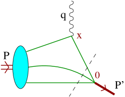
Figure 1: Schematic structure of the light-cone sum rule for nucleon form factors (Ref. [28]). The corresponding correlator function is given in (2.5), and $P^{\prime}=P-q$.

$$T_{\mu}(P,q)=i\!\int\!d^{4}x\,e^{iqx}\left\langle 0\right|T\left[\eta(0)j_{\mu}(x)\right]\left|N(P)\right\rangle\,,$$ (2.5)

with $P$ and $q$ being the nucleon and photon momentum, respectively. Here $j_{\mu}$ is the electromagnetic current

$$j_{\mu}(x)=e_{u}\bar{u}(x)\gamma_{\mu}u(x)+e_{d}\bar{d}(x)\gamma_{\mu}d(x)\,,$$ (2.6)

and in this work we choose the interpolating nucleon current of the form

$$\eta(x)=\varepsilon^{abc}\left[u^{a}(x)\;\Gamma_{1}u^{b}(x)\right]\;\Gamma_{2}\;d^{c}(x)\,,$$ (2.7)

where $a,b,c$ are colour indices. Here the generic expression (2.7) actually corresponds to the proton current, while the neutron current is obtained by replacing $u\leftrightarrow-d$. Specially, for Ioffe current [48]

$$\Gamma_{1}=C\gamma_{\lambda}\,,\qquad\Gamma_{2}=\gamma_{5}\gamma^{\lambda}\,,$$ (2.8)

with $C$ being the charge conjugation matrix. Other choices for $\eta(x)$ were discussed in, for example, Ref. [28], and Ioffe current was singled out as a most promising candidate for reliable sum rules.

2.3 Nucleon matrix element of the three-quark operator

Nucleon distribution amplitudes refer to nucleon-to-vacuum matrix elements of nonlocal operators built of quark and gluon fields at light-like separations, $x^{2}=0$.

We are interested in the three-quark matrix element

$$4\left\langle 0\right|\varepsilon^{abc}u^{a^{\prime}}_{\alpha}(a_{1}x)[a_{1}x,a_{0}x]_{a^{\prime}a}u^{b^{\prime}}_{\beta}(a_{2}x)[a_{2}x,a_{0}x]_{b^{\prime}b}d^{c^{\prime}}_{\gamma}(a_{3}x)[a_{3}x,a_{0}x]_{c^{\prime}c}\left|N(P,\lambda)\right\rangle$$ (2.9)

where

$$[x,y]={\cal P}\mbox{exp}[ig\int_{0}^{1}dt(x-y)_{\mu}A^{\mu}(tx-(1-t)y)]$$ (2.10)

is a gauge factor which we will suppress in the following, while $\alpha$,$\beta$,$\gamma$ are Dirac indices and $P^{2}=M_{N}^{2}$ with $M_{N}$ being the mass of the nucleon, i.e., proton mass for the three-quark matrix element considered above. Neutron case proceeds equivalently ($u\leftrightarrow d$). Actually, in this work all results are expressed in terms of proton quantities but the neutron case is easy to derive from these (in the end results, it comes basically to the replacement $e_{u}\leftrightarrow e_{d}$).

For the general Lorentz decomposition we introduce a convenient shorthand notation [49]

$$4\left\langle 0\right|\varepsilon^{abc}u_{\alpha}^{a}(a_{1}x)u_{\beta}^{b}(a_{2}x)d_{\gamma}^{c}(a_{3}x)\left|N(P,\lambda)\right\rangle=\sum\limits_{i}{\cal F}^{(i)}(\{a_{k}\},P\cdot x)\;X^{(i)}_{\alpha\beta}Y^{(i)}_{\gamma}\,,$$ (2.11)

where ${\cal F}^{(i)}\in\{{\cal S}_{1},{\cal S}_{2},{\cal P}_{1},{\cal P}_{2},{\cal V}_{1},\ldots,{\cal V}_{6},{\cal A}_{1},\ldots,{\cal A}_{6},{\cal T}_{1},\ldots,{\cal T}_{8}\}$ are invariant functions of $P\cdot x$, while $X^{(i)}_{\alpha\beta}$ and $Y^{(i)}_{\gamma}$ are Dirac structures which can be read from Ref. [28].

The structures $Y^{(i)}_{\gamma}$ contain nucleon spinor $N_{\gamma}$ and we note that

$$(X^{(i)})^{T}=\left\{\begin{array}[]{l}X^{(i)}\mbox{ for }{\cal F}^{(i)}\in\{{\cal V}_{j},{\cal T}_{j}\}\\ -X^{(i)}\mbox{ for }{\cal F}^{(i)}\in\{{\cal S}_{j},{\cal P}_{j},{\cal A}_{j}\}\end{array}\right.\,.$$ (2.12)

The functions ${\cal F}^{(i)}$ are not of a definite twist and they satisfy

$${\cal F}^{(i)}(a_{1}P\cdot x,a_{2}P\cdot x,a_{3}P\cdot x)=\left\{\begin{array}[]{l}{\cal F}^{(i)}(a_{2}P\cdot x,a_{1}P\cdot x,a_{3}P\cdot x)\mbox{ for }{\cal F}^{(i)}\in\{{\cal V}_{j},{\cal T}_{j}\}\\ -{\cal F}^{(i)}(a_{2}P\cdot x,a_{1}P\cdot x,a_{3}P\cdot x)\mbox{ for }{\cal F}^{(i)}\in\{{\cal S}_{j},{\cal P}_{j},{\cal A}_{j}\}\end{array}\right.\,.$$ (2.13)

Additional, ${\cal O}(x^{2})$ terms can be added to (2.11) but will not be explicitly considered here (see Ref. [28] instead).

2.3.1 Light-cone kinematics

For the twist classification it is convenient to go to infinite momentum frame and introduce a light-like vector $z_{\mu}$ by the condition

$$q\cdot z=0\,,\qquad z^{2}=0$$ (2.14)

as well as the second light-like vector

$$p_{\mu}=P_{\mu}-\frac{1}{2}\,z_{\mu}\frac{M_{N}^{2}}{P\cdot z}\,,~{}~{}~{}~{}~{}p^{2}=0\,,$$ (2.15)

so that $P\to p$ if the nucleon mass can be neglected, $M_{N}\to 0$. The projector onto the directions orthogonal to $p$ and $z$, is given by

$$g^{\perp}_{\mu\nu}=g_{\mu\nu}-\frac{1}{pz}(p_{\mu}z_{\nu}+p_{\nu}z_{\mu}).$$ (2.16)

In turn, $a_{\perp}$ denotes the generic component of $a_{\mu}$ orthogonal to $z$ and $p$, and thus the photon momentum can be written as

$$q_{\mu}=q_{\bot\mu}+z_{\mu}\frac{P\cdot q}{P\cdot z}\,,$$ (2.17)

where the use has been made of $p\cdot q=P\cdot q$ and $p\cdot z=P\cdot z$.

Assume for a moment that the nucleon moves in the positive ${\bf e_{z}}$ direction, then $p^{+}$ and $z^{-}$ are the only nonvanishing components of $p$ and $z$, respectively. The infinite momentum frame can be visualised as the limit $p^{+}\sim Q\to\infty$ with fixed $P\cdot z=p\cdot z\sim 1$ where $Q$ is the large scale in the process. Expanding the matrix element in powers of $1/p^{+}$ introduces the power counting in $Q$. In this language, twist counts the suppression in powers of $p^{+}$.

Similarly, the nucleon spinor $N_{\gamma}(P,\lambda)$ has to be decomposed in “large” and “small” components as

$$N_{\gamma}(P,\lambda)=(\Lambda^{+}+\Lambda^{-})N_{\gamma}(P,\lambda)=N^{+}_{\gamma}(P,\lambda)+N^{-}_{\gamma}(P,\lambda)\,,$$ (2.18)

where we introduce two projection operators

$$\Lambda^{+}=\frac{\!\not\!{p}\!\!\not\!{z}}{2p\cdot z}\quad,\quad\Lambda^{-}=\frac{\!\not\!{z}\!\!\not\!{p}}{2p\cdot z}$$ (2.19)

that project onto the “plus” and “minus” components of the spinor. Using the explicit expressions for $N(P)$ it is easy to see that $\Lambda^{+}N=N^{+}\sim\sqrt{p^{+}}$ while $\Lambda^{-}N=N^{-}\sim 1/\sqrt{p^{+}}$.

2.3.2 Twist decomposition

The twist decomposition of the nucleon-to-vacuum matrix element can be written in a form

$$4\left\langle 0\right|\varepsilon^{abc}u_{\alpha}^{a}(a_{1}x)u_{\beta}^{b}(a_{2}x)d_{\gamma}^{c}(a_{3}x)\left|N(P,\lambda)\right\rangle=\sum\limits_{i}F^{(i)}(\{a_{k}\},P\cdot x)\;W^{(i)}_{\alpha\beta}V^{(i)}_{\gamma}\,,$$ (2.20)

where $F^{(i)}\in\{S_{1},S_{2},P_{1},P_{2},V_{1},\ldots,V_{6},A_{1},\ldots,A_{6},T_{1},\ldots,T_{8}\}$ represent now nucleon distribution amplitudes (DAs) and functions of definite twist:

twist-3 $$V_{1}$$, ,

twist-4 , , , , , , , ,

twist-5 , , , , , , , ,

twist-6 , ,

(2.21)

The Dirac structures $W^{(i)}_{\alpha\beta}$ and $V^{(i)}_{\gamma}$ can be read from Ref. [28], and $V^{(i)}_{\gamma}$ contain the $N_{\gamma}^{+}$ or $N_{\gamma}^{-}$ projections of the nucleon spinor.

The functions ${\cal F}^{(i)}$ and $F^{(i)}$ are related by [28]

$$\begin{array}[]{ll}{\cal S}_{1}=S_{1}&2P\cdot x{\cal S}_{2}=S_{1}-S_{2}\\ {\cal P}_{1}=P_{1}&2P\cdot x{\cal P}_{2}=P_{2}-P_{1}\\ {\cal V}_{1}=V_{1}&2P\cdot x{\cal V}_{2}=V_{1}-V_{2}-V_{3}\\ 2{\cal V}_{3}=V_{3}&\ldots\\ \ldots&\\ {\cal A}_{1}=A_{1}&2P\cdot x{\cal A}_{2}=-A_{1}+A_{2}-A_{3}\\ 2{\cal A}_{3}=A_{3}&\ldots\\ \ldots&\\ {\cal T}_{1}=T_{1}&2P\cdot x{\cal T}_{2}=T_{1}+T_{2}-2T_{3}\\ \ldots&\end{array}$$ (2.22)

and each DA $F^{(i)}\in V_{j},A_{j},T_{j},S_{j},P_{j}$ can be represented as

$$F^{(i)}(\{a_{k}\},P\cdot x)=\int\!{\cal D}x\,e^{-iP\cdot x\sum_{j}x_{j}a_{j}}F(\{x_{i}\})\,,$$ (2.23)

where the functions $F^{(i)}(x_{i})$ depend on the dimensionless variables $x_{i},\,0<x_{i}<1,\sum_{i}x_{i}=1$ which correspond to the longitudinal momentum fractions carried by the quarks inside the nucleon. The integration measure is defined as

$${}\int\!{\cal D}x=\!\int_{0}^{1}\!\!\!dx_{1}dx_{2}dx_{3}\,\delta(x_{1}+x_{2}+x_{3}-1)\,.\hskip 14.22636pt\phantom{-}$$ (2.24)

Analogously to (2.13), the functions $F^{(i)}(\{x_{k}\})$ poses the following symmetry properties

$$F^{(i)}(x_{1},x_{2},x_{3})=\left\{\begin{array}[]{l}F^{(i)}(x_{2},x_{1},x_{3})\mbox{ for }F^{(i)}\in\{V_{j},T_{j}\}\\ -F^{(i)}(x_{2},x_{1},x_{3})\mbox{ for }F^{(i)}\in\{S_{j},P_{j},A_{j}\}\end{array}\right.\,.$$ (2.25)

According to (2.22), the functions ${\cal F}^{(i)}$ can be written in terms of nucleon DAs $F^{(i)}$ as

$${\cal F}^{(i)}(\{a_{k}\},P\cdot x)=\frac{1}{(2P\cdot x)^{n}}f(F^{(i)}(\{a_{k}\},P\cdot x))\,,\quad n\in\{0,1,2\}\,,$$ (2.26)

where $f$ is a linear combination of $F^{(i)}$. In addition, from (2.11) and Ref. [28] one can read off the dependence of Dirac structures $X^{(i)}$ and $Y^{(i)}$ on $x$-coordinates:

$$X^{(i)}Y^{(i)}\sim 1\mbox{ or }x_{\kappa}\mbox{ or }x_{\kappa}x_{\rho}\,.$$ (2.27)

Taking into account (2.26) and (2.27) the terms from (2.11) can be classified according to

$$n=0$$ and , , , , , , ,

and , , , , , , , , , , ,

and , , ,

(2.28)

After ${\cal F}^{(i)}$ functions are replaced by $F^{(i)}$ and the Fourier transform (2.23) is employed, one ends up with corresponding three types of integrals which in LO take the form:

$$1. \int d^{4}x\;\int\frac{d^{4}k_{\rm in}}{(2\pi)^{4}}\;e^{i(q+k_{\rm in})\cdot x}\int{\cal D}u\;e^{-iP\cdot x\sum_{j}u_{j}a_{j}}\;[F^{(i)}(\{u_{k}\})\ldots]$$

$$2. \int d^{4}x\;\int\frac{d^{4}k_{\rm in}}{(2\pi)^{4}}\;e^{i(q+k_{\rm in})\cdot x}\int{\cal D}u\;e^{-iP\cdot x\sum_{j}u_{j}a_{j}}\;\frac{x_{\kappa}}{(2P\cdot x)}\;[F^{(i)}(\{u_{k}\})\ldots]$$

$$3. \int d^{4}x\;\int\frac{d^{4}k_{\rm in}}{(2\pi)^{4}}\;e^{i(q+k_{\rm in})x}\int{\cal D}u\;e^{-iP\cdot x\sum_{j}u_{j}a_{j}}\;\frac{x_{\kappa}x_{\rho}}{(2P\cdot x)^{2}}\;[F^{(i)}(\{u_{k}\})\ldots]\,,\quad$$ (2.29)

with $k_{in}$ being the momentum of the quark propagator. Similar but slightly more complicated integrals appear at NLO.

The first integral in (2.29), corresponding to the first case in (2.28), simplifies trivially to

$$\int\frac{d^{4}k_{\rm in}}{(2\pi)^{4}}\ \int{\cal D}u\;(2\pi)^{4}\delta^{(4)}(q+k_{\rm in}-P\sum_{j}u_{j}a_{j})[F^{(i)}(\{u_{k}\})\ldots]$$

$$\quad=\int{\cal D}u\;[F^{(i)}(\{u_{k}\})\ldots]_{k_{\rm in}=P\sum_{j}u_{j}a_{j}-q}\;\,,$$ (2.30)

It is convenient to introduce the notation

$$A(u_{1},u_{2},u_{3})\otimes B(u_{1},u_{2},u_{3})=\int{\cal D}u\,A(u_{1},u_{2},u_{3})\,B(u_{1},u_{2},u_{3})\,.$$ (2.31)

and thus such contribution to the correlation function (2.5) can be expressed, both at LO and higher-orders, by a convolution

$$T_{\mu}=\sum\limits_{i}{\cal M}_{\mu}^{(i)}(\{u_{k}\})\otimes F^{(i)}(\{u_{k}\})\,.$$ (2.32)

In order to evaluate the other two integrals from (2.29) one employs

$$\int d^{4}x\;x_{\kappa}\;e^{i(q+k_{\rm in}-P\sum_{j}u_{j}a_{j})\cdot x} = -i\frac{\partial}{\partial k_{\rm in}^{\kappa}}\left((2\pi)^{4}\delta^{(4)}(q+k_{\rm in}-P\sum_{j}u_{j}a_{j})\right)\,,$$

$$\int d^{4}x\;x_{\kappa}x_{\rho}\;e^{i(q+k_{\rm in}-P\sum_{j}u_{j}a_{j})\cdot x} = \frac{\partial}{\partial k_{\rm in}^{\kappa}}\frac{\partial}{\partial k_{\rm in}^{\rho}}\left((2\pi)^{4}\delta^{(4)}(q+k_{\rm in}-P\sum_{j}u_{j}a_{j})\right)\,,\qquad$$ (2.33)

as well as partial integration, but we will leave out here further details.

2.4 Derivation of LCSR

Equating the correlation function (2.5) results in several invariant functions that can be separated by the appropriate projections. Lorentz structures that are most useful for writing the LCSRs are usually those containing the maximum power of the large momentum $p^{+}\sim p\cdot z$. Hence, for the Ioffe current, we define the invariant functions ${\cal A}$ and ${\cal B}$ by

$$z^{\mu}\Lambda_{+}T_{\mu} = (p\cdot z)\left\{M_{N}\mathcal{A}+\!\not\!q_{\perp}\mathcal{B}\right\}N^{+}(P)\,,$$ (2.34)

where $\mathcal{A}$ and $\mathcal{B}$ depend on the Lorentz-invariants $Q^{2}=-q^{2}$ and $P^{\prime 2}=(P-q)^{2}$.

2.4.1 Correlation function versus form factors

Next we relate the correlation function (2.5) to nucleon form factors. The correlation function can be written as

$$T_{\mu}(P,q)=\frac{1}{M_{N}^{2}-P^{\prime 2}}\sum_{s}\left\langle 0\right|\eta(0)\left|N(P^{\prime},s)\right\rangle\left<N(P^{\prime},s)|j_{\mu}^{\rm em}(0)|N(P)\right>+\ldots$$ (2.35)

where the leading term is the nucleon contribution and the dots stand for higher resonances.

Inserting (2.1) and the matrix element of the Ioffe current

$$\left\langle 0\right|\eta(0)\left|N(P)\right\rangle=\lambda_{1}\,M_{N}\,N(P)\,,$$ (2.36)

using $\sum_{s}N(P)\bar{N}(P)=\not\!P+M_{N}$, and taking the projection suitable for our calculation, one obtains

$$\Lambda_{+}\,z_{\mu}\,T^{\mu}=\frac{\lambda_{1}}{M_{N}^{2}-P^{\prime 2}}\left\{2(P\cdot z)\,M_{N}\,F_{1}(Q^{2})\,N^{+}(P)+(P\cdot z)\,F_{2}(Q^{2})\,\not\!q_{\perp}\,N^{+}(P)\right\}+\,\cdots$$ (2.37)

Now, by comparing (2.37) and (2.34) one gets

$$\frac{2\lambda_{1}}{M_{N}^{2}-P^{\prime 2}}F_{1}(Q^{2})+\cdots = {\cal A}(Q^{2},P^{\prime 2})\,,$$

$$\frac{\lambda_{1}}{M_{N}^{2}-P^{\prime 2}}F_{2}(Q^{2})+\cdots = {\cal B}(Q^{2},P^{\prime 2})\,.$$ (2.38)

2.4.2 Light-cone sum rules

We can calculate ${\cal A}$ and ${\cal B}$ perturbatively in terms of quarks and gluons.

Furthermore, (see, for example, Ref. [24]) we can formally write a dispersion relation

$${\cal A}(Q^{2},P^{\prime 2}) = \frac{1}{\pi}\int_{0}^{\infty}ds\,\frac{{\rm Im}{\cal A}(Q^{2},s)}{s-P^{\prime 2}}\,,$$

$${\cal B}(Q^{2},P^{\prime 2}) = \frac{1}{\pi}\int_{0}^{\infty}ds\,\frac{{\rm Im}{\cal B}(Q^{2},s)}{s-P^{\prime 2}}\,.$$ (2.39)

Now, by making use of the quark-hadron duality (analogously to, for example, Ref. [50]) the effects of higher-resonances cancel between the left and right hand side of (2.38) and one ends up with the sum rules

$$\frac{2\lambda_{1}}{M_{N}^{2}-P^{\prime 2}}F_{1}(Q^{2}) = \frac{1}{\pi}\int_{0}^{s_{0}}ds\,\frac{{\rm Im}{\cal A}(Q^{2},s)}{s-P^{\prime 2}}\,,$$

$$\frac{\lambda_{1}}{M_{N}^{2}-P^{\prime 2}}F_{2}(Q^{2}) = \frac{1}{\pi}\int_{0}^{s_{0}}ds\,\frac{{\rm Im}{\cal B}(Q^{2},s)}{s-P^{\prime 2}}\,,$$ (2.40)

where $s_{0}$ is a convenient mass cut-off, which in our case corresponds to the continuum threshold taken at Roper resonance, $s_{0}\approx(1.5{\rm GeV})^{2}$ [28], and which eliminates contributions other than nucleon (continuum subtraction).

In practice, one can imagine to perform a power expansion of expression (2.40) in the variable $P^{\prime 2}$. To improve the convergence of this expansion one then employs Borel transformation

$$\mbox{B}_{X\to M_{B}^{2}}[F(X)]=\lim_{n\to\infty}\frac{(-X)^{n}}{\Gamma(n)}\left[\frac{d^{n}}{dX^{n}}F(X)\right]_{|X|=nM_{B}^{2},\,X\to\infty}\,,$$ (2.41)

and of particular use in further calculation is a Borel transformation (see, for example, [24, 51])

$$\mbox{B}_{X\to M_{B}^{2}}[1/(x-X)]=e^{-x/M_{B}^{2}}/M_{B}^{2}\,.$$ (2.42)

Hence, taking a Borel transformation of the left and right hand-side of Eqs. (2.40) in variables $X=P^{\prime 2}$, one ends up with the sum rules

$$F_{1}(Q^{2}) = \frac{1}{2\lambda_{1}\pi}\int_{0}^{s_{0}}ds\;e^{(-s+M_{N}^{2})/M_{B}^{2}}\;{\rm Im}{\cal A}(Q^{2},s)\,,$$

$$F_{2}(Q^{2}) = \frac{1}{\lambda_{1}\pi}\int_{0}^{s_{0}}ds\;e^{(-s+M_{N}^{2})/M_{B}^{2}}\;{\rm Im}{\cal B}(Q^{2},s)\,.$$ (2.43)

For the Borel mass $M_{B}$ which can be viewed as a matching scale of hadronic and partonic part of the calculation, we, as in Ref. [28], take $M_{B}^{2}=2$ GeV².

We note here that in this draft we adopt the derivation of the sum rules based on the dispersion relations (2.39) and Borel transformation (2.42) which then lead to (2.43). After calculating the needed imaginary parts and performing the necessary integrals it can be shown that this approach is equivalent to the one employed in Ref. [28] but perhaps more suitable for NLO calculations.

The imaginary parts of the functions of interest are listed in App. D.

2.5 $M_{N}$ dependence

Due to calculational difficulties at NLO order, it is convenient to perform an expansion in mass $M_{N}$, i.e., schematically, the contributions to the correlation function can be presented by

$$\frac{A+M_{N}B+CM_{N}^{2}+...}{a+bM_{N}^{2}}=\frac{A}{a}+M_{N}\frac{B}{a}+{\cal O}(M_{N}^{2})\,.$$ (2.44)

The first term corresponds to taking $M_{N}=0$, while the first two terms correspond to taking $M_{N}^{2}=0$ while retaining $M_{N}$ proportional terms in the calculation. In calculating NLO contribution we will try to investigate these two cases. In loop calculations additional $\ln(M_{N}^{2})$ terms appear, and thus in the $M_{N}^{2}=0$ approximation collinear singularities.

The $M_{N}$-dependence of the general Lorentz decomposition of the nucleon matrix element (2.11) can be summarized as

$$M_{N}^{0}$$-proportional , ,

-proportional , , , , , , , ,

-proportional , , , , , , , ,

-proportional , ,

(2.45)

Obviously for $M_{N}=0$ only the terms proportional to ${\cal F}^{(i)}\in\{{\cal V}_{1},{\cal A}_{1},{\cal T}_{1}\}$ will contribute to $T_{\mu}$. But for $M_{N}\neq 0$ the contributions proportional to ${\cal F}^{(i)}\in\{{\cal V}_{1},{\cal A}_{1},{\cal T}_{1}\}$ will contain also $M_{N}^{n}$-proportional ($n\neq 0$) terms.

3 LO contributions

As a preparation and necessary ingredient of the NLO calculation, in this section we discuss in detail LO contributions to correlator function $T_{\mu}$ (2.5). We present the complete twist-3 and twist-4 results and devote the last part of the section to the analysis and discussion of gauge invariance.

3.1 General structure and properties of LO contributions

Using general Lorentz decomposition of the nucleon matrix element of the three-quark operator given in Eq. (2.11) and interpolating nucleon current of the form (2.7), one obtains the general form of the LO contribution to the correlation function (2.5)

$$T_{\mu}^{\rm LO} = -\frac{1}{4}\int d^{4}xe^{iq\cdot x}\int\frac{d^{4}k_{\rm in}}{(2\pi)^{4}}e^{ik_{\rm in}\cdot x}\sum\limits_{i}$$

$$\times\left\{e_{u}\;{\cal F}^{(i)}(P\cdot x,0,0)\;{\rm Tr}\left[X^{(i)}\Gamma_{1}\frac{\not\!k_{\rm in}+m_{u}}{k_{\rm in}^{2}-m_{u}^{2}}\gamma_{\mu}\right]\;\Gamma_{2}Y^{(i)}_{\gamma}\right.$$

$$\left.\quad+e_{u}\;{\cal F}^{(i)}(0,P\cdot x,0)\;{\rm Tr}\left[\left(X^{(i)}\right)^{T}\Gamma_{1}\frac{\not\!k_{\rm in}+m_{u}}{k_{\rm in}^{2}-m_{u}^{2}}\gamma_{\mu}\right]\;\Gamma_{2}Y^{(i)}_{\gamma}\right.$$

$$\left.\quad+e_{d}\;{\cal F}^{(i)}(0,0,P\cdot x)\;{\rm Tr}\left[\left(X^{(i)}\right)^{T}\Gamma_{1}\right]\;\Gamma_{2}\frac{\not\!k_{\rm in}+m_{d}}{k_{\rm in}^{2}-m_{d}^{2}}\gamma_{\mu}Y^{(i)}_{\gamma}\right\}\,,$$

and in following we neglect quark masses $m_{u}=m_{d}=0$. Taking into account the form of $X^{(i)}$ it is easy to see that only the terms proportional to ${\cal F}^{(i)}\in\{{\cal V}_{j},{\cal A}_{j}\}$ contribute if Ioffe current, i.e., $\Gamma_{1}=C\gamma_{\lambda}$ and $\Gamma_{2}=\gamma_{5}\gamma^{\lambda}$, is taken for interpolating nucleon current. Namely, the matrices $X^{(i)}$ (see Ref. [28]) proportional to ${\cal F}^{(i)}\in\{{\cal V}_{j},{\cal A}_{j}\}$ and ${\cal F}^{(i)}\in\{{\cal S}_{j},{\cal P}_{j},{\cal T}_{j}\}$ consist of odd and even number of $\gamma$ matrices, respectively, and hence the traces from (LABEL:eq:LOgen) vanish in latter case.

The contribution corresponding to the first case of (2.28) takes the form

$$T_{\mu}^{{\rm LO}} = -\frac{1}{4}\sum\limits_{i}\int{\cal D}u\,N^{(i)}\,F^{(i)}(\{u_{k}\})$$

$$\times\left\{e_{u}\;{\rm Tr}\left[X^{(i)}\Gamma_{1}\frac{u_{1}\not\!P-\not\!q}{(u_{1}P-q)^{2}}\gamma_{\mu}\right]\;\Gamma_{2}Y^{(i)}_{\gamma}\right.$$

$$\left.\quad+e_{u}\;{\rm Tr}\left[\left(X^{(i)}\right)^{T}\Gamma_{1}\frac{u_{2}\not\!P-\not\!q}{(u_{2}P-q)^{2}}\gamma_{\mu}\right]\;\Gamma_{2}Y^{(i)}_{\gamma}\right.$$

$$\left.\quad+e_{d}\;{\rm Tr}\left[\left(X^{(i)}\right)^{T}\Gamma_{1}\right]\;\Gamma_{2}\frac{u_{3}\not\!P-\not\!q}{(u_{3}P-q)^{2}}\gamma_{\mu}Y^{(i)}_{\gamma}\right\}\,,$$

and using (2.32) we can write

$$T_{\mu}^{{\rm LO}} = \sum\limits_{i}{\cal M}^{{\rm LO},(i)}(\{u_{k}\})\,\otimes\,F^{(i)}(\{u_{k}\})\,,$$ (3.3)

where from comparison with (LABEL:eq:LOcase1) the definition of ${\cal M}^{{\rm LO},(i)}(\{u_{k}\})$ is obvious. As explained in Sec. 2.3.2, for the other two cases listed in (2.28) slightly more involved formulas appear.

For Ioffe current (2.8), there are two twist-3 contributions ($F^{(i)}\in\{V_{1},A_{1}\}$) calculable by (LABEL:eq:LOcase1) with $N^{(i)}=1$, and steaming from

$${\cal F}^{(i)}$$

(3.4)

Furthermore, when using Ioffe current, there are the two twist-4 contributions ($F^{(i)}\in\{V_{3},A_{3}\}$) calculable using (LABEL:eq:LOcase1) with $N^{(i)}=1/2$, and two twist-4 contributions ($F^{(i)}\in\{V_{2},A_{2}\}$) corresponding to the more involved second case of (2.28). These contributions stem from

$${\cal F}^{(i)}$$

(3.5)

Our main interest in this work are LO and NLO contributions to twist-3 contributions and the generalization to other first case contributions. Hence, we do not discuss in detail the calculation of second and third case LO contributions from (2.28), nor higher-twist contributions, but rather refer to [28] and references therein.

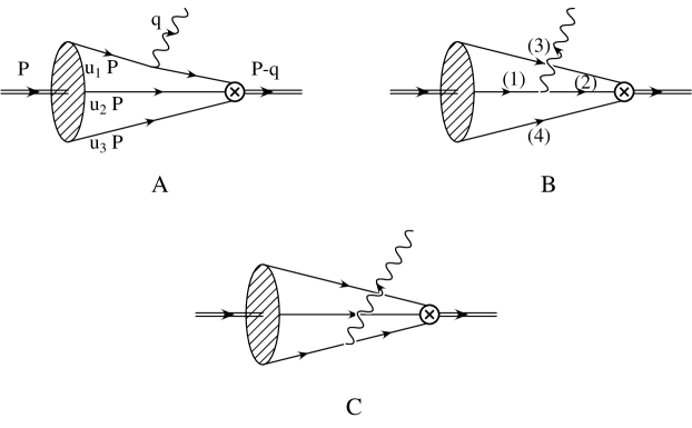
Figure 2: LO diagrams contributing to the correlation function (2.5). On diagram B the nomenclature for NLO diagrams is sketched.

In order to simplify higher-order calculation it is convenient to extract the Feynman rules and perform the calculation in momentum space. The three terms contributing to (LABEL:eq:LOgen) correspond actually to three Feynman diagrams presented on Fig. 2.

The Feynman rules for the contributions corresponding to first case of (2.28) are listed in Appendix A. Using these rules it is trivial to write down the contributions corresponding to the LO diagrams in Fig. 2. As it should, these contributions agree with corresponding terms in Eq. (LABEL:eq:LOcase1) and

$$T_{\mu}^{{\rm LO}} = \sum\limits_{i}\left(T_{\mu}^{A,(i)}+T_{\mu}^{B,(i)}+T_{\mu}^{C,(i)}\right)\,.$$ (3.6)

Taking into account (2.12) it is easy to see that

$${\cal M}_{\mu}^{B,(i)}(u_{1},u_{2},u_{3})=\left\{\begin{array}[]{l}{\cal M}_{\mu}^{A,(i)}(u_{2},u_{1},u_{3})\quad\mbox{for}\quad F^{(i)}\in\{V_{1},V_{3}\}\\ -{\cal M}_{\mu}^{A,(i)}(u_{2},u_{1},u_{3})\quad\mbox{for}\quad F^{(i)}\in\{A_{1},A_{3}\}\\ \end{array}\right.\,.$$ (3.7)

It is also obvious that ${\cal M}^{C,A1}(\{u_{k}\})={\cal M}^{C,A3}(\{u_{k}\})=0$.

Hence for the first case of (2.28) one can write

$${\cal M}^{{\rm LO},(i)}(\{u_{k}\}) = -\frac{1}{4}N^{(i)}$$ (3.8)

$$\times\left\{e_{u}\;{\rm Tr}\left[\left(\frac{u_{1}\not\!P-\not\!q}{(u_{1}P-q)^{2}}\pm\frac{u_{2}\not\!P-\not\!q}{(u_{2}P-q)^{2}}\right)\gamma_{\mu}X^{(i)}(C\gamma_{\lambda})\right]\;\gamma_{5}\gamma^{\lambda}Y^{(i)}_{\gamma}\right.$$

$$\left.+e_{d}\;{\rm Tr}\left[X^{(i)}(C\gamma_{\lambda})\right]\;\gamma_{5}\gamma^{\lambda}\frac{u_{3}\not\!P-\not\!q}{(u_{3}P-q)^{2}}\gamma_{\mu}Y^{(i)}_{\gamma}\right\}\,,$$

where $``+^{\prime\prime}$ sign in the first term corresponds to $F^{(i)}\in\{V_{1},V_{3}\}$ and $``-^{\prime\prime}$ sign to $F^{(i)}\in\{A_{1},A_{3}\}$. Finally, note that, since we are interested in NLO calculation in which dimensional regularization will be employed, one has to use $D=4-2\epsilon$ dimensions also at LO.

3.2 Twist-3 results

Table 1: LO twist-3 contributions corresponding to the diagrams of Fig. 2. The contributions ${\cal M}_{\mu}^{B,(i)}$ can be obtained using (3.7).

${\cal M}_{\mu}^{A,V1}$	$\displaystyle\frac{e_{u}}{Q^{2}+2u_{1}P\cdot q-u_{1}^{2}M_{N}^{2}}\left[P_{\mu}\left(2u_{1}M_{N}-\not\!q\right)-q_{\mu}M_{N}+\gamma_{\mu}\left(P\cdot q-u_{1}M_{N}^{2}\right)\right]$
${\cal M}_{\mu}^{A,A1}$	$\displaystyle\frac{e_{u}}{Q^{2}+2u_{1}P\cdot q-u_{1}^{2}M_{N}^{2}}\left[P_{\mu}\not\!q-q_{\mu}M_{N}-\gamma_{\mu}P\cdot q+\gamma_{\mu}\not\!qM_{N}\right]$
${\cal M}_{\mu}^{C,V1}$	$\displaystyle\frac{e_{d}}{Q^{2}+2u_{3}P\cdot q-u_{3}^{2}M_{N}^{2}}\left[2P_{\mu}\not\!q-2q_{\mu}M_{N}+\gamma_{\mu}\left(-2P\cdot q+u_{3}M_{N}^{2}\right)+\gamma_{\mu}\not\!qM_{N}\right]$
${\cal M}_{\mu}^{C,A1}$	0

In Table 1 we present the LO twist-3 contributions to diagrams displayed on Fig. 2. The complete LO contributions to amplitudes ${\cal M}_{\mu}^{{\rm LO},(i)}$ are given by

$${\cal M}_{\mu}^{{\rm LO},(i)}(u_{1},u_{2},u_{3}) = {\cal M}_{\mu}^{A,(i)}(u_{1},u_{2},u_{3})+{\cal M}_{\mu}^{B,(i)}(u_{1},u_{2},u_{3})+{\cal M}_{\mu}^{C,(i)}(u_{1},u_{2},u_{3})$$

$$= {\cal M}_{\mu}^{A,(i)}(u_{1},u_{2},u_{3})\pm{\cal M}_{\mu}^{A,(i)}(u_{2},u_{1},u_{3})+{\cal M}_{\mu}^{C,(i)}(u_{1},u_{2},u_{3})\,,$$

where $``+^{\prime\prime}$ sign in the second line corresponds to $V_{1}$ contributions and $``-^{\prime\prime}$ sign to $A_{1}$ contributions. The correlation function is given by (3.3) and taking into account the DA symmetry properties (2.25), one obtains

$$\left({\cal M}_{\mu}^{A,(i)}(u_{1},u_{2},u_{3})\pm{\cal M}_{\mu}^{A,(i)}(u_{2},u_{1},u_{3})\right)\otimes F^{(i)}(u_{1},u_{2},u_{3})$$ (3.10)

$$\qquad= 2\,{\cal M}_{\mu}^{A,(i)}(u_{1},u_{2},u_{3})\otimes F^{(i)}(u_{1},u_{2},u_{3})\,,$$

but it is advantageous for NLO calculation to leave full $u_{1}$ and $u_{2}$ dependence of the amplitude ${\cal M}$.

Our LO as well as NLO results for $T_{\mu}$ can be presented in terms of six invariant functions which multiply the Lorentz structures $P_{\mu}M_{N}$, $P_{\mu}\not\!\!q$, $q_{\mu}M_{N}$, $q_{\mu}\not\!\!q$, $\gamma_{\mu}$, and $\gamma_{\mu}\not\!\!qM_{N}$. Thus it is advantageous for future calculations to present the results in a form

$${\cal M}_{\mu}^{X,(i)}(\{u_{k}\}) = C^{X,(i)}_{P_{\mu}M_{N}}(\{u_{k}\})\;P_{\mu}M_{N}+C^{X,(i)}_{P_{\mu}\not q}(\{u_{k}\})\;P_{\mu}\not\!q$$

$$+C^{X,(i)}_{q_{\mu}M_{N}}(\{u_{k}\})\;q_{\mu}M_{N}+C^{X,(i)}_{q_{\mu}\not q}(\{u_{k}\})\;q_{\mu}\not\!q$$

$$+C^{X,(i)}_{\gamma_{\mu}}(\{u_{k}\})\;\gamma_{\mu}+C^{X,(i)}_{\gamma_{\mu}\not qM_{N}}(\{u_{k}\})\;\gamma_{\mu}\not\!qM_{N}\,.$$

The corresponding LO twist-3 coefficients are given in Table 2.

Table 2: LO coefficients (LABEL:eq:Mcoeff) corresponding to $V_{1}$ and $A_{1}$ DAs.

$C^{{\rm LO},V1}_{P_{\mu}M_{N}}$	$\displaystyle\left(\frac{2u_{1}e_{u}}{Q^{2}+2u_{1}P\cdot q-u_{1}^{2}M_{N}^{2}}+(u_{1}\leftrightarrow u_{2})\right)$
$C^{{\rm LO},V1}_{P_{\mu}\not q}$	$\displaystyle\left(\frac{-e_{u}}{Q^{2}+2u_{1}P\cdot q-u_{1}^{2}M_{N}^{2}}+(u_{1}\leftrightarrow u_{2})\right)+\frac{2e_{d}}{Q^{2}+2u_{3}P\cdot q-u_{3}^{2}M_{N}^{2}}$
$C^{{\rm LO},V1}_{q_{\mu}M_{N}}$	$\displaystyle\left(\frac{-e_{u}}{Q^{2}+2u_{1}P\cdot q-u_{1}^{2}M_{N}^{2}}+(u_{1}\leftrightarrow u_{2})\right)+\frac{-2e_{d}}{Q^{2}+2u_{3}P\cdot q-u_{3}^{2}M_{N}^{2}}$
$C^{{\rm LO},V1}_{q_{\mu}\not q}$	$0$
$C^{{\rm LO},V1}_{\gamma_{\mu}}$	$\displaystyle\left(\frac{e_{u}(P\cdot q-u_{1}M_{N}^{2})}{Q^{2}+2u_{1}P\cdot q-u_{1}^{2}M_{N}^{2}}+(u_{1}\leftrightarrow u_{2})\right)+\frac{e_{d}(-2P\cdot q+u_{3}M_{N}^{2})}{Q^{2}+2u_{3}P\cdot q-u_{3}^{2}M_{N}^{2}}$
$C^{{\rm LO},V1}_{\gamma_{\mu}\not qM_{N}}$	$\displaystyle\frac{e_{d}}{Q^{2}+2u_{3}P\cdot q-u_{3}^{2}M_{N}^{2}}$
$C^{{\rm LO},A1}_{P_{\mu}M_{N}}$	$0$
$C^{{\rm LO},A1}_{P_{\mu}\not q}$	$\displaystyle\left(\frac{e_{u}}{Q^{2}+2u_{1}P\cdot q-u_{1}^{2}M_{N}^{2}}-(u_{1}\leftrightarrow u_{2})\right)$
$C^{{\rm LO},A1}_{q_{\mu}M_{N}}$	$\displaystyle\left(\frac{-e_{u}}{Q^{2}+2u_{1}P\cdot q-u_{1}^{2}M_{N}^{2}}-(u_{1}\leftrightarrow u_{2})\right)$
$C^{{\rm LO},A1}_{q_{\mu}\not q}$	$0$
$C^{{\rm LO},A1}_{\gamma_{\mu}}$	$\displaystyle\left(\frac{-P\cdot q\,e_{u}}{Q^{2}+2u_{1}P\cdot q-u_{1}^{2}M_{N}^{2}}-(u_{1}\leftrightarrow u_{2})\right)$
$C^{{\rm LO},A1}_{\gamma_{\mu}\not qM_{N}}$	$\displaystyle\left(\frac{e_{u}}{Q^{2}+2u_{1}P\cdot q-u_{1}^{2}M_{N}^{2}}-(u_{1}\leftrightarrow u_{2})\right)$

Finally, we present the results for the invariant functions ${\mathcal{A}}$ and ${\mathcal{B}}$ defined in (2.34). Multiplying $T_{\mu}$ with $z^{\mu}\Lambda_{+}$ the invariant functions ${\mathcal{A}}$ and ${\mathcal{B}}$ are projected. It is easy to see that these correspond to the invariant functions multiplying $P_{\mu}M_{N}$ and $P_{\mu}\not\!q$, and thus

$${\mathcal{A}}^{\rm twist-3}(Q^{2},(P-q)^{2}) = C^{{\rm LO},V1}_{P_{\mu}M_{N}}(\{u_{k}\})\;\otimes\;V_{1}(\{u_{k}\})+C^{{\rm LO},A1}_{P_{\mu}M_{N}}(\{u_{k}\})\;\otimes\;A_{1}(\{u_{k}\})\,,$$

$${\mathcal{B}}^{\rm twist-3}(Q^{2},(P-q)^{2}) = C^{{\rm LO},V1}_{P_{\mu}\not\!q}(\{u_{k}\})\;\otimes\;V_{1}(\{u_{k}\})+C^{{\rm LO},A1}_{P_{\mu}\not\!q}(\{u_{k}\})\;\otimes\;A_{1}(\{u_{k}\})\,.$$

The results presented here are in agreement with the results from [28].

3.3 Twist-4 results

The twist-4 contributions corresponding to $V_{3}$ and $A_{3}$ are obtained analogously to the twist-3 results discussed in the preceding subsection. The LO coefficients corresponding to (LABEL:eq:Mcoeff) are given in Table 3. Note the dependence on $\epsilon=(4-D)/2$.

Table 3: LO coefficients (LABEL:eq:Mcoeff) corresponding to $V_{3}$ and $A_{3}$ DAs.

$C^{{\rm LO},V3}_{P_{\mu}M_{N}}$	$\displaystyle\left(\frac{-(3-\epsilon)u_{1}e_{u}}{Q^{2}+2u_{1}P\cdot q-u_{1}^{2}M_{N}^{2}}+(u_{1}\leftrightarrow u_{2})\right)+\frac{-2(1-\epsilon)u_{3}e_{d}}{Q^{2}+2u_{3}P\cdot q-u_{3}^{2}M_{N}^{2}}$
$C^{{\rm LO},V3}_{P_{\mu}\not q}$	$0$
$C^{{\rm LO},V3}_{q_{\mu}M_{N}}$	$\displaystyle\left(\frac{(3-\epsilon)e_{u}}{Q^{2}+2u_{1}P\cdot q-u_{1}^{2}M_{N}^{2}}+(u_{1}\leftrightarrow u_{2})\right)+\frac{2(1-\epsilon)e_{d}}{Q^{2}+2u_{3}P\cdot q-u_{3}^{2}M_{N}^{2}}$
$C^{{\rm LO},V3}_{q_{\mu}\not q}$	$0$
$C^{{\rm LO},V3}_{\gamma_{\mu}}$	$\displaystyle\left(\frac{u_{1}M_{N}^{2}e_{u}}{Q^{2}+2u_{1}P\cdot q-u_{1}^{2}M_{N}^{2}}+(u_{1}\leftrightarrow u_{2})\right)+\frac{-\epsilon u_{3}M_{N}^{2}e_{d}}{Q^{2}+2u_{3}P\cdot q-u_{3}^{2}M_{N}^{2}}$
$C^{{\rm LO},V3}_{\gamma_{\mu}\not qM_{N}}$	$\displaystyle\left(\frac{-e_{u}}{Q^{2}+2u_{1}P\cdot q-u_{1}^{2}M_{N}^{2}}+(u_{1}\leftrightarrow u_{2})\right)+\frac{\epsilon e_{d}}{Q^{2}+2u_{3}P\cdot q-u_{3}^{2}M_{N}^{2}}$
$C^{{\rm LO},A3}_{P_{\mu}M_{N}}$	$\displaystyle\left(\frac{u_{1}(1-\epsilon)e_{u}}{Q^{2}+2u_{1}P\cdot q-u_{1}^{2}M_{N}^{2}}-(u_{1}\leftrightarrow u_{2})\right)$
$C^{{\rm LO},A3}_{P_{\mu}\not q}$	$0$
$C^{{\rm LO},A3}_{q_{\mu}M_{N}}$	$\displaystyle\left(\frac{-(1-\epsilon)e_{u}}{Q^{2}+2u_{1}P\cdot q-u_{1}^{2}M_{N}^{2}}-(u_{1}\leftrightarrow u_{2})\right)$
$C^{{\rm LO},A3}_{q_{\mu}\not q}$	$0$
$C^{{\rm LO},A3}_{\gamma_{\mu}}$	$\displaystyle\left(\frac{-(1-\epsilon)u_{1}M_{N}^{2}e_{u}}{Q^{2}+2u_{1}P\cdot q-u_{1}^{2}M_{N}^{2}}-(u_{1}\leftrightarrow u_{2})\right)$
$C^{{\rm LO},A3}_{\gamma_{\mu}\not qM_{N}}$	$\displaystyle\left(\frac{(1-\epsilon)e_{u}}{Q^{2}+2u_{1}P\cdot q-u_{1}^{2}M_{N}^{2}}-(u_{1}\leftrightarrow u_{2})\right)$

Furthermore, without going into much detail, we present also the contributions corresponding to ${\cal V}_{2},{\cal A}_{2}$ – see (3.5). We therefore introduce the shorthand notation

$$V_{123}=V_{1}-V_{2}-V_{3},$$

$$A_{123}=-A_{1}+A_{2}-A_{3}.$$ (3.14)

Furthermore, as in [28], we use the definition

$$\widetilde{F}(u_{l}) \equiv \int_{1}^{u_{l}}dv_{l}\int_{0}^{1-v_{l}}du_{m}\,F(\{v_{l},u_{m},1-v_{l}-u_{m}\})\,.$$ (3.15)

Here $F$ is the nucleon DA or the combination of nucleon DAs that depends on three valence quark momentum fractions, and the integration over one momentum fraction has already been performed using $\delta(1-v_{l}-u_{m}-u_{k})$. Note that in this notation, which follows closely Ref. [28], $\widetilde{F}(u_{l})$ is not a simple function of $u_{l}$ and that the form of the function itself depends on $u_{l}=u_{1}$, $u_{2}$ or $u_{3}$, i.e., whether $u_{l}$ corresponds to the momentum fraction of the first u-quark, second u-quark or d-quark. Note that $\widetilde{F}(u_{1})=\pm\widetilde{F}(u_{2})$ for $F(u_{1},u_{2},u_{3})=\pm F(u_{2},u_{1},u_{3})$, respectively.

The function $\widetilde{F}(u_{i})$ depends on only one momentum fraction and enters the expression analogous to (2.32), but that expression contains the integration with amplitude ${\cal M}(u_{i})$ only over one remaining momentum fraction $u_{i}$. This property holds in LO (where the dependence on $u_{1}$, $u_{2}$ and $u_{3}$ is clearly separated) while in NLO the expressions will be more involved. For tabulated LO contributions see Table 4.

Table 4: LO coefficients analogous to (LABEL:eq:Mcoeff) and corresponding to $\widetilde{V}_{123}(u_{i})$ and $\widetilde{A}_{123}(u_{i})$ (3.14-3.15): $\int_{0}^{1}du_{i}C^{{\rm LO},F_{123}}_{\cdots}(u_{i})\widetilde{F}_{123}(u_{i})$  for $u_{i}\in\{u_{1},u_{2},u_{3}\}$.

$\{C^{{\rm LO},V_{123}}_{P_{\mu}M_{N}}(u_{i})\}$	$\displaystyle\left\{\frac{e_{u}((2-\epsilon)Q^{2}+2(1-\epsilon)u_{1}P\cdot q-(1-\epsilon)M_{N}^{2}u_{1}^{2})}{(Q^{2}+2u_{1}P\cdot q-u_{1}^{2}M_{N}^{2})^{2}}\,,(u_{1}\leftrightarrow u_{2})\,,\right.$
	$\displaystyle\left.-\frac{e_{d}(-2\epsilon\,Q^{2}+4(1-\epsilon)u_{3}P\cdot q+2(\epsilon-1)u_{3}^{2}M_{N}^{2})}{(Q^{2}+2u_{3}P\cdot q-u_{3}^{2}M_{N}^{2})^{2}}\right\}$
$\{C^{{\rm LO},V_{123}}_{P_{\mu}\not q}(u_{i})\}$	$\displaystyle\left\{\frac{e_{u}u_{1}M_{N}^{2}}{(Q^{2}+2u_{1}P\cdot q-u_{1}^{2}M_{N}^{2})^{2}}\,,(u_{1}\leftrightarrow u_{2})\,,\frac{2e_{d}u_{3}M_{N}^{2}}{(Q^{2}+2u_{3}P\cdot q-u_{3}^{2}M_{N}^{2})^{2}}\right\}$
$\{C^{{\rm LO},V_{123}}_{q_{\mu}M_{N}}(u_{i})\}$	$\displaystyle\left\{\frac{e_{u}(2P\cdot q-u_{1}M_{N}^{2})}{(Q^{2}+2u_{1}P\cdot q-u_{1}^{2}M_{N}^{2})^{2}}\,,(u_{1}\leftrightarrow u_{2})\,,\frac{e_{d}\,(4P\cdot q-2u_{3}M_{N}^{2})}{(Q^{2}+2u_{3}P\cdot q-u_{3}^{2}M_{N}^{2})^{2}}\right\}$
$\{C^{{\rm LO},V_{123}}_{q_{\mu}\not q}(u_{i})\}$	$\displaystyle\left\{\frac{-e_{u}M_{N}^{2}}{(Q^{2}+2u_{1}P\cdot q-u_{1}^{2}M_{N}^{2})^{2}}\,,(u_{1}\leftrightarrow u_{2})\,,\frac{-2e_{d}M_{N}^{2}}{(Q^{2}+2u_{3}P\cdot q-u_{3}^{2}M_{N}^{2})^{2}}\right\}$
$\{C^{{\rm LO},V_{123}}_{\gamma_{\mu}}(u_{i})\}$	$\displaystyle\left\{\frac{-e_{u}M_{N}^{2}(Q^{2}+u_{1}P\cdot q)}{(Q^{2}+2u_{1}P\cdot q-u_{1}^{2}M_{N}^{2})^{2}}\,,(u_{1}\leftrightarrow u_{2})\,,\frac{-e_{d}\,\epsilon M_{N}^{2}}{Q^{2}+2u_{3}P\cdot q-u_{3}^{2}M_{N}^{2}}\right\}$
$\{C^{{\rm LO},V_{123}}_{\gamma_{\mu}\not qM_{N}}(u_{i})\}$	$\displaystyle\left\{\frac{e_{u}(-P\cdot q+u_{1}M_{N}^{2})}{(Q^{2}+2u_{1}P\cdot q-u_{1}^{2}M_{N}^{2})^{2}}\,,(u_{1}\leftrightarrow u_{2})\,,0\right\}$
$\{C^{{\rm LO},A_{123}}_{P_{\mu}M_{N}}(u_{i})\}$	$\displaystyle\left\{\frac{e_{u}\,(-\epsilon Q^{2}+2(1-\epsilon)u_{1}P\cdot q-(1-\epsilon)u_{1}^{2}M_{N}^{2})}{(Q^{2}+2u_{1}P\cdot q-u_{1}^{2}M_{N}^{2})^{2}}\,,-(u_{1}\leftrightarrow u_{2})\,,0\right\}$
$\{C^{{\rm LO},A_{123}}_{P_{\mu}\not q}(u_{i})\}$	$\displaystyle\left\{(\frac{-e_{u}u_{1}M_{N}^{2}}{(Q^{2}+2u_{1}P\cdot q-u_{1}^{2}M_{N}^{2})^{2}}\,,-(u_{1}\leftrightarrow u_{2})\,,0\right\}$
$\{C^{{\rm LO},A_{123}}_{q_{\mu}M_{N}}(u_{i})\}$	$\displaystyle\left\{\frac{e_{u}(-2P\cdot q+u_{1}M_{N}^{2})}{(Q^{2}+2u_{1}P\cdot q-u_{1}^{2}M_{N}^{2})^{2}}\,,-(u_{1}\leftrightarrow u_{2})\,,0\right\}$
$\{C^{{\rm LO},A_{123}}_{q_{\mu}\not q}(u_{i})\}$	$\displaystyle\left\{\frac{e_{u}M_{N}^{2}}{(Q^{2}+2u_{1}P\cdot q-u_{1}^{2}M_{N}^{2})^{2}}\,,-(u_{1}\leftrightarrow u_{2})\,,0\right\}$
$\{C^{{\rm LO},A_{123}}_{\gamma_{\mu}}(u_{i})\}$	$\displaystyle\left\{\frac{-e_{u}M_{N}^{2}(-\epsilon Q^{2}+(1-2\epsilon)u_{1}P\cdot q-(1-\epsilon)u_{1}^{2}M_{N}^{2})}{(Q^{2}+2u_{1}P\cdot q-u_{1}^{2}M_{N}^{2})^{2}}\,,-(u_{1}\leftrightarrow u_{2})\,,0\right\}$
$\{C^{{\rm LO},A_{123}}_{\gamma_{\mu}\not qM_{N}}(u_{i})\}$	$\displaystyle\left\{\frac{e_{u}(P\cdot q-u_{1}M_{N}^{2})}{(Q^{2}+2u_{1}P\cdot q-u_{1}^{2}M_{N}^{2})^{2}}\,,-(u_{1}\leftrightarrow u_{2})\,,0\right\}$

The contributions to functions ${\cal A}$ and ${\cal B}$ are given by (E.3) and (E.8).

3.4 Gauge invariance

Due to the presence of nucleon interpolation current, the condition of gauge invariance takes for the correlator function (2.5) the form

$$q_{\mu}T^{\mu}=Q_{\eta}\,\left\langle 0\right|\eta(0)\left|N(P)\right\rangle\,,$$ (3.16)

with $Q_{\eta}=1$ for the proton interpolation current and full electromagnetic current (2.6), while when one considers $e_{u}$- and $e_{d}$-proportional parts of the electromagnetic current separately $Q_{\eta}=2e_{u}=4/3$ and $Q_{\eta}=e_{d}=-1/3$, respectively (in the neutron case, as usual, $e_{u}\leftrightarrow e_{d}$). Furthermore for Ioffe current we have

$$\left\langle 0\right|\eta(0)\left|N(P)\right\rangle=\lambda_{1}\,M_{N}\,N(P)\,.$$ (3.17)

In the preceding subsections we have presented the complete LO twist-3 and twist-4 contributions to the correlator function, i.e., in contrast to Ref. [28], not just the terms corresponding to the functions of interest ${\cal A}$ and ${\cal B}$. This enables us to check the gauge invariance. By making use of the results given in Tables 2, 3 and 4 one can easily see that for $M_{N}^{2}\neq 0$ the gauge invariance does not hold, i.e., that (3.16) is not satisfied, for separate ${\cal F}^{(i)}$-proportional terms nor for separate twists.

Let us consider the expansion in $M_{N}$ given as outlined in Sec. 2.5.

In the $M_{N}=0$ approximation, taking into account (3.17), the gauge condition (3.16) takes the simple form

$$q_{\mu}T^{\mu}=0\,.$$ (3.18)

In this approximation only twist-3 contributions proportional to $V_{1}$ and $A_{1}$ exist. As can be easily seen from LO results listed in Table 2, these contributions are separately gauge invariant, as well as, $e_{u}$ and $e_{d}$ parts separately. The same condition applies and holds for NLO and higher-order contributions.

Furthermore, we have checked the gauge invariance of the LO results in the $M_{N}^{2}=0$ but $M_{N}\neq 0$ approximation to which $V_{1}$, $V_{3}$, $V_{2}$, $A_{1}$, $A_{3}$, and $A_{2}$ DAs contribute. This approximation corresponds to the first two terms in Eq. (2.44). Using the LO results given in Tables 2, 3 and 4 and taking $M_{N}^{2}=0$, one can show that

$$q_{\mu}T^{\mu}=Q_{\eta}\,\lambda_{1}\,M_{N}\,N(P)\,$$ (3.19)

is satisfied when the sum of all contributing terms is taken into account (i.e., both twist-3 and twist-4 contributions) and the asymptotic forms of twist-3 DAs are used. There are no, at least at this order of expansion in $M_{N}$, conditions on twist-4 DAs.

Hence, gauge invariance can be satisfied order by order in the expansion in $M_{N}$ (2.44) with possibly some additional conditions on the form of DAs. For the check of higher order terms in $M_{N}$ one should calculate the complete LO higher-twist contributions to the correlation function.

4 NLO contributions

We are finally ready to address in this section the NLO contributions to the correlator function $T_{\mu}$ (2.5). We will present the results obtained in $M_{N}=0$ approximation (corresponding to the first term in (2.44)), discuss the problems encountered in $M_{N}\neq 0$ but $M_{N}^{2}=0$ approximation (corresponding to the first two terms in (2.44)), and outline the obstacles present in general $M_{N}^{2}\neq 0$ calculation.

4.1 Topological structure

Three LO diagrams displayed in Fig. 2 lead to $30$ NLO diagrams. The nomenclature we use can be deduced from Fig. 2 (diagram B): at NLO the gluon is attached in all possible ways. Typical NLO diagrams are presented in Fig. 3.

The contributions of $Bij$ diagrams one can obtain from the contribution of $Aij$ diagrams by $u_{1}\leftrightarrow u_{2}$ exchange analogous to (3.7). The similar relation connects diagrams $C24$ and $C23$, as well as, $C14$ and $C13$. Taking all this into account, there are 8 more complicated diagrams to calculate ($A12$, $A23$, $A24$, $A13$, $A14$, $C12$, $C24$, $C14$) and the rest are either proportional to LO ($X11$, $X33$, $X44$, $X22$, $X34$) or obtainable from above mentioned symmetries.

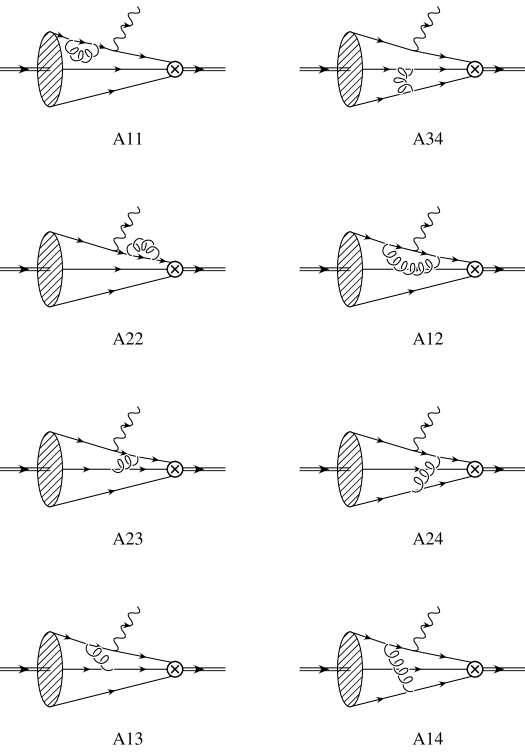
Figure 3: Typical NLO diagrams. The contributions of “self-energy“ diagrams $A33$ and $A44$ is equal to the contribution of diagram $A11$. Diagrams $Bij$ and $Cij$ are similar to the ones presented above, while the nomenclature is sketched on Fig. 2.

Our calculation is performed in Feynman gauge. The colour factors were calculated using usual $SU(N_{C}=3)$-algebra relations. In the first group of diagrams where gluon couples to the same quark line the colour factor is $C_{F}=(N_{C}^{2}-1)/(2N_{C})=4/3$ while in the second in which gluon connects two different lines colour factors equal $(-C_{B})=-(N_{C}+1)(2N_{C})=-2/3$. As mentioned in App. A, since we are describing nucleon as colour singlet state of three quarks ($\varepsilon^{abc}$), the $N_{C}=3$ choice is enforced.

4.2 Using dimensional regularization and resolving $\gamma_{5}$ ambiguity

In the following NLO calculation we take

$$P^{2}=M_{N}^{2}=0$$ (4.1)

and consider diagrams with massless on-shell external legs. Hence, apart from UV divergences the IR divergences of collinear type appear (there are no “true” IR divergences). Both divergences are regularized using dimensional regularization in

$$D=4-2\epsilon$$

dimensions.

We introduce the abbreviations

$$\Gamma_{UV}(\epsilon) = \Gamma(\epsilon)\frac{\Gamma(1-\epsilon)\Gamma(1-\epsilon)}{\Gamma(1-2\epsilon)}(4\pi)^{\epsilon}=\frac{1}{\epsilon}-\gamma+\ln(4\pi)+O(\epsilon)\,,$$ (4.2a)

$$\Gamma_{IR}(\epsilon) = \Gamma(1+\epsilon)\frac{\Gamma(-\epsilon)\Gamma(1-\epsilon)}{\Gamma(1-2\epsilon)}(4\pi)^{\epsilon}=\frac{1}{-\epsilon}+\gamma-\ln(4\pi)+O(\epsilon)\,.$$ (4.2b)

The first $\Gamma$ function on the right-hand side of Eqs. (4.2) originates from the loop momentum integration, while the integration over Feynman parameters produces $\Gamma$s collected in a fraction. Consequently, the singularity contained in $\Gamma(\epsilon)$ appearing in (4.2a) is of UV origin, while the singularity contained in $\Gamma(-\epsilon)$ appearing in (4.2b) is of infrared (IR), i.e., collinear, origin. From $\Gamma(z)\Gamma(1-z)=\pi/\sin\pi z$ one can see that to all orders in $\epsilon$

$$\Gamma_{UV}(\epsilon)=-\Gamma_{IR}(\epsilon)\,.$$ (4.3)

Nevertheless, we find it useful to keep track of the origin of the UV and collinear singularities (for details, see also Refs. [52, 53]).

In dimensional regularization the “trivial” self-energy diagrams ($X11$, $X33$, $X44$), as well as, “trivial” 3-point integral ($X34$) vanish if one allows that UV and IR divergences to cancel. However, as mentioned above, we adopt here an approach of consistent tracking of UV and collinear singularities, and their separate removal by renormalization and factorization, respectively.

Additionally, when calculating the contributions to $T_{\mu}$ corresponding to $A_{i}$ distribution amplitudes we encounter $\gamma_{5}$-ambiguity – see App. B for details. In these cases the general Lorentz decomposition (2.11) and the choice of nucleon interpolating current (2.7) lead to the appearance of the traces with one $\gamma_{5}$ matrix. At NLO these traces contain contracting $\gamma$ matrices and, as such, trace $\gamma_{5}$-ambiguity. Moreover, after the trace operation is performed one is left with one or more Levi-Civita tensors which get contracted with additional $\gamma$ matrices. Hence, the ambiguity related to the use of Chisholm identity is also present.

We choose to use the naive-$\gamma_{5}$ scheme [54]. We could choose to use HV scheme [55, 56] but then we would have to know or somehow calculate the terms which remove “spurious“ anomalies violating Ward identities. Moreover we would have to use HV scheme also for the calculation of otherwise nonproblematic contributions corresponding to $V_{i}$.

We remember that the choice of general decomposition (2.11) is not unique and that using Fierz transformations one could get the representation in which there is no trace and as such no $\gamma_{5}$ ambiguity (no trace ambiguity and no appearance of Levi-Civita tensor). Hence, the intermediate appearance of the problems with $\gamma_{5}$ are caused by our choice of the Lorentz decomposition of the nucleon matrix element and by the choice of the interpolating current. One can, for example, use the Lorentz decomposition of the form $X_{\gamma\beta}^{(i)}Y_{\alpha}^{(i)}$ (see App. A in Ref. [25] for useful relations) which when used with (2.7) does not lead to the appearance of the trace. But the price to pay when using this decomposition are much larger expressions, $\epsilon$ proportional terms at LO even for $V_{1}$ and $A_{1}$ etc..

Nevertheless, that possibility lead us to the correct way to handle contractions using Chisholm identity: ”follow” the fermion line (as usual, that means to go opposite the fermion line) and always perform the contraction of the Levi-Civita with the ”last” $\gamma$ matrix (with an open index) on the $d$ line. The generalized recipe follows that one should write also the traces as a part of an expression obtained following the fermion lines – remember that the essence of trace ambiguity is loosing the cyclicity of the trace – see App. B.

When calculating NLO contributions in $M_{N}=0$ approximation, we have used the gauge invariance (3.16) as a check and a help to resolve $\gamma_{5}$-ambiguity. After adopting this simple recipe – to write all parts of expression ”following” the fermion lines: opposite d-line, along u-line ($C\cdots C^{-1}$ present - see App. A), opposite u-line, and to perform all evaluations obeying that order – we obtain the gauge invariant NLO results as one should.

4.3 Twist-3 and $M_{N}=0$

Let us first investigate the approximation in which we neglect nucleon mass completely and take consistently throughout the calculation $M_{N}=0$. As can be seen from (2.45), the general Lorentz decomposition of nucleon matrix element of three quark operator (2.11) has for $M_{N}=0$ only three terms: the ones proportional to ${\cal V}_{1}$, ${\cal A}_{1}$, and ${\cal T}_{1}$. The tensor contributions vanish for our choice of interpolating nucleon current, and we are left with two contributions convoluted with $V_{1}$ and $A_{1}$:

$$\left.T_{\mu}\right|_{M_{N}=0}={\cal M}_{\mu}^{V1}(u_{1},u_{2},u_{3})\otimes V_{1}(u_{1},u_{2},u_{3})+{\cal M}_{\mu}^{A1}(u_{1},u_{2},u_{3})\otimes A_{1}(u_{1},u_{2},u_{3})\,.$$ (4.4)

As explained in, for example, Ref. [25], since $V_{1}$ and $A_{1}$ have different symmetry properties (see (2.25)), they can be combined together to define a single independent twist-3 nucleon distribution amplitude:

$$\Phi_{3}(x_{1},x_{2},x_{3})=V_{1}(x_{1},x_{2},x_{3})-A_{1}(x_{1},x_{2},x_{3})\,.$$ (4.5)

Now, by taking into account that the convolution of symmetric and antisymmetric functions gives 0, as well as, relation (4.5) and symmetry properties (2.25), one can write (4.4) as

$$\left.T_{\mu}\right|_{M_{N}=0} = \frac{1}{2}\left({\cal M}_{\mu}^{V1}(u_{1},u_{2},u_{3})+{\cal M}_{\mu}^{V1}(u_{2},u_{1},u_{3})\right)\otimes V_{1}(u_{1},u_{2},u_{3})$$ (4.6)

$$+\frac{1}{2}\left({\cal M}_{\mu}^{A1}(u_{1},u_{2},u_{3})-{\cal M}_{\mu}^{A1}(u_{2},u_{1},u_{3})\right)\otimes A_{1}(u_{1},u_{2},u_{3})$$

$$= \frac{1}{2}\left({\cal M}_{\mu}^{V1}(u_{1},u_{2},u_{3})+{\cal M}_{\mu}^{V1}(u_{2},u_{1},u_{3})-{\cal M}_{\mu}^{A1}(u_{1},u_{2},u_{3})+{\cal M}_{\mu}^{A1}(u_{1},u_{2},u_{3})\right)$$

$$\otimes\,\Phi_{3}(u_{1},u_{2},u_{3})$$

$$= {\cal M}_{\mu}^{\Phi}(u_{1},u_{2},u_{3})\otimes\Phi_{3}(u_{1},u_{2},u_{3})\,.$$

From (4.6) the definition of ${\cal M}_{\mu}^{\Phi}$ is obvious.

4.3.1 Renormalization and factorization of collinear singularities: $\Phi_{3}$

We start here with the explanation of renormalization procedure for (4.6) in which $T_{\mu}$ is given in terms of convolution of only two functions ${\cal M}_{\mu}^{\Phi}(u_{1},u_{2},u_{3})$ and $\Phi_{3}(u_{1},u_{2},u_{3})$. We follow closely Ref. [52].

The amplitude ${\cal M}_{\mu}^{\Phi}(u_{1},u_{2},u_{3})$ is of the general form

$${\cal M}=Z_{\rm curr}\;\left[{\cal M}^{{\rm LO}}+\frac{\alpha_{s}}{4\pi}{\cal M}^{{\rm NLO}}+\cdots\right]\,,$$ (4.7a)

where

$${\cal M}^{{\rm LO}} = a_{0}+\epsilon a_{1}+{\cal O}(\epsilon^{2})\,,$$ (4.7b)

$${\cal M}^{{\rm NLO}} = \left\{\Gamma_{UV}(\epsilon)\left[b_{0}^{UV}+\epsilon b_{1}^{UV}+{\cal O}(\epsilon^{2})\right]+\Gamma_{IR}(\epsilon)\left[b_{0}^{IR}+\epsilon b_{1}^{IR}+{\cal O}(\epsilon^{2})\right]\right\}\left(\frac{\mu^{2}}{Q^{2}}\right)^{\epsilon}\,,$$

and ${\cal M}^{{\rm LO}}$ and ${\cal M}^{{\rm NLO}}$ are calculated from LO and NLO diagrams from Figs. 2 and 3, respectively.

The bare coupling constant $\alpha_{s}$ can be defined in terms of the running coupling constant $\alpha_{s}(\mu_{R}^{2})$ as

$$\alpha_{s}=\alpha_{s}(\mu_{R}^{2})\left(1-\frac{\alpha_{s}(\mu_{R}^{2})}{4\pi}\beta_{0}\frac{1}{\epsilon}\right)\left(\frac{\mu_{R}^{2}}{\mu^{2}}\right)^{\epsilon}\left[\epsilon\Gamma_{UV}(\epsilon)\right]^{-1}\,,$$ (4.8)

and to the order we are calculating this essentially means that the bare coupling is replaced by the renormalized one and no singularities are removed as yet.

The expansion of the amplitude ${\cal M}$ takes the form

$${\cal M}=Z_{\rm curr}\;\left\{{\cal M}^{{\rm LO}}+\frac{\alpha_{s}(\mu_{R}^{2})}{4\pi}{\hat{\cal M}}^{{\rm NLO}}+\cdots\right\}\,,$$ (4.9a)

where

$${\cal M}^{{\rm LO}} = a_{0}+\epsilon a_{1}+{\cal O}(\epsilon^{2})\,,$$ (4.9b)

$${\hat{\cal M}}^{{\rm NLO}} = \left\{\frac{1}{\epsilon}\left[b_{0}^{UV}+\epsilon b_{1}^{UV}+{\cal O}(\epsilon^{2})\right]+\frac{1}{-\epsilon}\left[b_{0}^{IR}+\epsilon b_{1}^{IR}+{\cal O}(\epsilon^{2})\right]\right\}\left(\frac{\mu_{R}^{2}}{Q^{2}}\right)^{\epsilon}\,.\qquad$$ (4.9c)

In our case the coefficients of the $1/\epsilon$ poles of UV origin, i.e., $b_{0}^{UV}$, are removed by renormalization of the nucleon interpolating current (Ioffe current in this calculation). For that purpose $Z_{\rm curr}$ has been introduced and it is of the form

$$Z_{\rm curr}=1-\alpha_{s}(\mu_{R,1}^{2})\frac{C_{\rm curr}^{(1)}}{\epsilon}+{\cal O}(\alpha_{s}^{2})\,,$$ (4.10)

where $\mu_{R,1}^{2}$ is a scale at which the nucleon interpolation current is renormalized. The change of the scale of the renormalization constant is given by

$$\alpha_{s}(\mu^{2})=\left(\frac{\mu_{R}^{2}}{\mu^{2}}\right)^{\epsilon}\alpha_{s}(\mu_{R}^{2})\left[1+{\cal O}(\alpha_{s})\right]$$ (4.11)

Hence, ${\cal M}$ takes the form

$${\cal M}={\cal M}^{{\rm LO}}+\frac{\alpha_{s}(\mu_{R}^{2})}{4\pi}{\widehat{\cal M}}^{{\rm NLO}}+\cdots\,,$$ (4.12a)

where

$${\cal M}^{{\rm LO}} = a_{0}+\epsilon a_{1}+{\cal O}(\epsilon^{2})\,,$$ (4.12b)

and

$${\widehat{\cal M}}^{{\rm NLO}}$$ (4.12c)

$$= \left\{\frac{1}{\epsilon}\left[\left(b_{0}^{UV}-C_{\rm curr}^{(1)}\,a_{0}\left(\frac{Q^{2}}{\mu_{R,1}^{2}}\right)^{\epsilon}\right)+\epsilon\left(b_{1}^{UV}-C_{\rm curr}^{(1)}\,a_{1}\left(\frac{Q^{2}}{\mu_{R,1}^{2}}\right)^{\epsilon}\right)+{\cal O}(\epsilon^{2})\right]\right.$$

$$\left.+\frac{1}{-\epsilon}\left[b_{0}^{IR}+\epsilon b_{1}^{IR}+{\cal O}(\epsilon^{2})\right]\right\}\left(\frac{\mu_{R}^{2}}{Q^{2}}\right)^{\epsilon}\,.$$

For

$$b_{0}^{UV}-C_{\rm curr}^{(1)}\,a_{0}=0$$ (4.13)

the $1/\epsilon$ poles of UV origin vanish, and as only signature of their existence the logarithms $C_{\rm curr}^{(1)}\,a_{0}\ln(\mu_{R,1}^{2}/Q^{2})$ will remain in the end result. Notice that we have shown here that in principle coupling constant renormalization and the renormalization of the current can be performed at different scales, $\mu_{R}^{2}$ and $\mu_{R,1}^{2}$. Generally, we write the amplitude ${\cal M}$ as an expansion in $\alpha_{s}(\mu_{R}^{2})$ and independent of $\mu_{R}^{2}$. The truncation of this series in actual calculation will introduce the dependence of the results on $\mu_{R}^{2}$ (frequently discussed in the literature).

The remaining collinear singularities get cancelled by the renormalization constant of the nucleon distribution amplitude. Namely,

$$T_{\mu}\left|{}_{M_{N}=0}\right. = {\cal M}_{\mu}^{\Phi}(u_{1},u_{2},u_{3})\otimes\,\Phi_{3}(u_{1},u_{2},u_{3})$$ (4.14)

$$= {\cal M}_{\mu}^{\Phi}(u_{1},u_{2},u_{3})\otimes\,Z_{\Phi}(u_{1},u_{2},u_{3};x_{1},x_{2},x_{3};\mu_{F}^{2})\otimes\,\Phi_{3}(x_{1},x_{2},x_{3};\mu_{F}^{2})$$

$$= {\cal M}_{\mu}^{\Phi}(x_{1},x_{2},x_{3};\mu_{F}^{2})\otimes\,\Phi_{3}(x_{1},x_{2},x_{3};\mu_{F}^{2})\,.$$

The renormalization constant $Z_{\Phi}$ is of the form

$$Z_{\Phi}(\{u_{k}\},\{x_{k}\};\mu_{F}^{2})=\delta(u_{1}-x_{1})\delta(u_{2}-x_{2})-\alpha_{s}(\mu_{F}^{2})\frac{V_{\Phi}^{(1)}(\{u_{k}\},\{x_{k}\})}{-\epsilon}+{\cal O}(\alpha_{s}^{2})\,,$$ (4.15)

where $V_{\Phi}^{(1)}$ is a leading term of the kernel of the evolution equation for twist-3 DA:

$$\mu^{2}\frac{\partial}{\partial\mu^{2}}\Phi_{3}(\{u_{k}\};\mu^{2})=V_{\Phi}(\{u_{k}\},\{x_{k}\};\mu^{2})\,\otimes\Phi_{3}(\{x_{k}\};\mu^{2})\,,$$ (4.16)

and

$$V_{\Phi}(\{u_{k}\};\{x_{k}\};\mu^{2})=\frac{\alpha_{s}(\mu^{2})}{4\pi}\,V_{\Phi}^{(1)}(\{u_{k}\};\{x_{k}\})+{\cal O}(\alpha_{s})\,.$$ (4.17)

The kernel $V_{\Phi}^{(1)}$ was given in Ref. [7] and confirmed, for example, by the calculation of anomalous dimensions in Ref. [57]. Here we present it in a convenient form

$$V^{(1)}_{\Phi}(\{u_{k}\},\{x_{k}\})$$ (4.23)

$$= -\frac{3}{2}C_{F}\delta(u_{1}-x_{1})\delta(u_{2}-x_{2})$$

$$+C_{F}\left\{\delta(u_{3}-x_{3})\left[\frac{u_{1}}{x_{1}}\frac{1}{x_{1}-u_{1}}\theta(x_{1}-u_{1})+\frac{u_{2}}{x_{2}}\frac{1}{x_{2}-u_{2}}\theta(x_{2}-u_{2})\right]+\left(\begin{array}[]{l}3\leftrightarrow 1\\ 3\leftrightarrow 2\end{array}\right)\right\}_{+}$$

$$+2C_{B}\left\{\delta(u_{3}-x_{3})\left[\frac{u_{1}}{x_{1}}\theta(x_{1}-u_{1})+\frac{u_{2}}{x_{2}}\theta(x_{2}-u_{2})\right]\frac{\delta_{h_{1}\bar{h}_{2}}}{u_{1}+u_{2}}+\left(\begin{array}[]{l}3\leftrightarrow 1\\ 3\leftrightarrow 2\end{array}\right)\right\}\,,$$

where $h_{i}=-\bar{h}_{i}$ is a helicity of quark $i$, while

$$\left\{F(\{u_{k}\},\{x_{k}\})\right\}_{+}=F(\{u_{k}\},\{x_{k}\})-\delta(u_{1}-x_{1})\delta(u_{2}-x_{2})\int{\cal D}zF(\{z_{k}\},\{x_{k}\})\,.$$ (4.24)

We stress that one should take $C_{F}=2C_{B}=4/3$. Furthermore, in (4.23) one has to take

$$\delta_{h_{1}\bar{h}_{2}}=1\,,\quad\delta_{h_{2}\bar{h}_{3}}=1\,,\quad\delta_{h_{1}\bar{h}_{3}}=0\,,$$ (4.25)

i.e., the helicities of the quarks correspond to

$$u_{\uparrow(\downarrow)}u_{\downarrow(\uparrow)}d_{\uparrow(\downarrow)}\,,$$ (4.26)

which is in agreement with App.C from Ref. [28].

For the finite amplitude ${\cal M}$ one then gets

$${\cal M}(\{x_{k}\};\mu_{F}^{2})=\left\{{\cal M}^{{\rm LO}}(\{x_{k}\})+\frac{\alpha_{s}(\mu_{R}^{2})}{4\pi}{\cal M}^{{\rm NLO}}(\{x_{k}\};\mu_{F}^{2},\mu_{R,1}^{2})+\cdots\right\}\,,$$ (4.27a)

where

$${\cal M}^{{\rm LO}}(\{x_{k}\}) = a_{0}+\epsilon a_{1}+{\cal O}(\epsilon^{2})\,,$$ (4.27b)

$${\cal M}^{{\rm NLO}}(\{x_{k}\};\mu_{F}^{2},\mu_{R,1}^{2})$$ (4.27c)

$$= \left\{\frac{1}{\epsilon}\left[\left(b_{0}^{UV}-C_{\rm curr}^{(1)}a_{0}\left(\frac{Q^{2}}{\mu_{R,1}^{2}}\right)^{\epsilon}\right)+\epsilon\left(b_{1}^{UV}-C_{\rm curr}^{(1)}a_{1}\left(\frac{Q^{2}}{\mu_{R,1}^{2}}\right)^{\epsilon}\right)+{\cal O}(\epsilon^{2})\right]\right.$$

$$\left.+\frac{1}{-\epsilon}\left[\left(b_{0}^{IR}-a_{0}\,\otimes V^{(1)}\left(\frac{Q^{2}}{\mu_{F}^{2}}\right)^{\epsilon}\right)+\epsilon\left(b_{1}^{IR}-a_{1}\otimes V^{(1)}\left(\frac{Q^{2}}{\mu_{F}^{2}}\right)^{\epsilon}\right)+{\cal O}(\epsilon^{2})\right]\right\}$$

$$\times\left(\frac{\mu_{R}^{2}}{Q^{2}}\right)^{\epsilon}\,,$$

where $\mu_{F}$ is a (usual) factorization scale and the collinear singularities cancel for

$$b_{0}^{IR}-a_{0}\,\otimes V^{(1)}=0\,.$$ (4.28)

With all singularities cancelled, we can now take the limit $\epsilon\rightarrow 0$ and finally obtain

$${\cal M}(\{x_{k}\};\mu_{F}^{2})=\left\{{\cal M}^{{\rm LO}}(\{x_{k}\})+\frac{\alpha_{s}(\mu_{R}^{2})}{4\pi}{\cal M}^{{\rm NLO}}(\{x_{k}\};\mu_{F}^{2},\mu_{R,1}^{2})+\cdots\right\}\,,$$ (4.29a)

with

$${\cal M}^{{\rm LO}}(\{x_{k}\}) = a_{0}\,,$$ (4.29b)

$${\cal M}^{{\rm NLO}}(\{x_{k}\};\mu_{F}^{2},\mu_{R,1}^{2}) = \left(b_{1}^{UV}-C_{\rm curr}^{(1)}a_{1}\right)-\left(b_{1}^{IR}-a_{1}\otimes V^{(1)}\right)$$ (4.29c)

$$+C_{\rm curr}^{(1)}a_{0}\ln(\mu_{R,1}^{2}/Q^{2})-a_{0}\otimes V^{(1)}\ln(\mu_{F}^{2}/Q^{2})\,.\quad$$

For Ioffe current

$$C_{\rm curr}^{(1)}=C_{\rm Ioffe}^{(1)}=2\,.$$ (4.30)

Furthermore, one can check in Table 1 that for our twist-3 results there are no $\epsilon$ proportional LO contribution (in contrast to, for example, twist-4 contributions) and $a_{1}=0$. Taking this into account along with the conditions for cancelling UV (4.13) and collinear singularities (4.28), simplifies the NLO result (4.29c) to

$${\cal M}^{{\rm NLO}}(\{x_{k}\};\mu_{F}^{2},\mu_{R,1}^{2})=b_{1}^{UV}-b_{1}^{IR}+b_{0}^{UV}\ln(\mu_{R,1}^{2}/Q^{2})-b_{0}^{IR}\ln(\mu_{F}^{2}/Q^{2})\,.$$ (4.31)

4.3.2 Renormalization and factorization of collinear singularities: $V_{1}$ and $A_{1}$

Although (4.6) and the analysis given in the preceding subsection are sufficient for obtaining twist-3 results, we now turn to renormalization procedure for $T_{\mu}$ expressed in terms of $V_{1}$ and $A_{1}$. i.e, as in (4.4):

$$\left.T_{\mu}\right|_{M_{N}=0}={\cal M}_{\mu}^{V1}(u_{1},u_{2},u_{3})\otimes V_{1}(u_{1},u_{2},u_{3})+{\cal M}_{\mu}^{A1}(u_{1},u_{2},u_{3})\otimes A_{1}(u_{1},u_{2},u_{3})\,.$$

The crucial difference in comparison to the preceding subsection is that $T_{\mu}$ is no longer expressed as just one convolution but rather as a sum of convolutions. As we shall see, there is a mixing between these terms. The procedure is similar to the one used in Ref. [58] and, although the finite results are the same as the ones in preceding subsection, the experience that we gain in this subsection should be very useful for the $M_{N}\neq 0$ case.

It is instructive to write (4.4) in a matrix form:

$$\left.T_{\mu}\right|_{M_{N}=0}=\left({\cal M}_{\mu}^{V1}(u_{1},u_{2},u_{3}),{\cal M}_{\mu}^{A1}(u_{1},u_{2},u_{3})\right)\otimes\left(\begin{array}[]{l}V_{1}(u_{1},u_{2},u_{3})\\ A_{1}(u_{1},u_{2},u_{3})\end{array}\right)\,.$$ (4.32)

Both ${\cal M}_{\mu}^{V1}$ and ${\cal M}_{\mu}^{A1}$ can be expanded as in (4.7) and the UV renormalization of these expressions proceeds the same way as explained in the previous subsection. One ends up with the UV-finite expressions of the form (4.12):

$${\cal M}_{\mu}^{V1}(\{u_{k}\}) = {\cal M}^{{\rm LO},V1}_{\mu}(\{u_{k}\})+\frac{\alpha_{s}(\mu_{R}^{2})}{4\pi}{\widehat{\cal M}}^{{\rm NLO},V1}_{\mu}(\{u_{k}\})+\cdots\,,$$

$${\cal M}_{\mu}^{A1}(\{u_{k}\}) = {\cal M}^{{\rm LO},A1}_{\mu}(\{u_{k}\})+\frac{\alpha_{s}(\mu_{R}^{2})}{4\pi}{\widehat{\cal M}}^{{\rm NLO},A1}_{\mu}(\{u_{k}\})+\cdots\,,$$ (4.33)

and the conditions (4.13) have to be satisfied, i.e.,

$$b_{0}^{UV,V1}-C_{\rm curr}^{(1)}\,a_{0}^{V1} = 0\,,$$

$$b_{0}^{UV,A1}-C_{\rm curr}^{(1)}\,a_{0}^{A1} = 0\,.$$ (4.34)

In order to cancel remaining collinear singularities one has to know the evolution kernels, i.e., renormalization constants, for $V_{1}$ and $A_{1}$ distributions amplitudes. One can probably derive it by additional one-loop calculation, or, as we will do here, make use of our knowledge of $V_{\Phi}$. Knowing the symmetry properties of $V_{1}$ and $A_{1}$ distribution amplitudes, we write $V_{\Phi}$ as

$$V_{\Phi}(\{u_{k}\};\{x_{k}\};\mu^{2}) = V_{V1,V1}(\{u_{k}\};\{x_{k}\};\mu^{2})+V_{V1,A1}(\{u_{k}\};\{x_{k}\};\mu^{2})$$ (4.35a)

$$+\,V_{A1,V1}(\{u_{k}\};\{x_{k}\};\mu^{2})+V_{A1,A1}(\{u_{k}\};\{x_{k}\};\mu^{2})\,,\quad$$

where

$$V_{V1,V1}(\{u_{k}\};\{x_{k}\};\mu^{2}) = \frac{1}{4}\left(V_{\Phi}(u_{1},u_{2},u_{3};x_{1},x_{2},x_{3};\mu^{2})+V_{\Phi}(u_{1},u_{2},u_{3};x_{2},x_{1},x_{3};\mu^{2})\right.$$

$$\left.+V_{\Phi}(u_{2},u_{1},u_{3};x_{1},x_{2},x_{3};\mu^{2})+V_{\Phi}(u_{2},u_{1},u_{3};x_{2},x_{1},x_{3};\mu^{2})\right)\,,$$

$$V_{V1,A1}(\{u_{k}\};\{x_{k}\};\mu^{2}) = \frac{1}{4}\left(V_{\Phi}(u_{1},u_{2},u_{3};x_{1},x_{2},x_{3};\mu^{2})-V_{\Phi}(u_{1},u_{2},u_{3};x_{2},x_{1},x_{3};\mu^{2})\right.$$

$$\left.+V_{\Phi}(u_{2},u_{1},u_{3};x_{1},x_{2},x_{3};\mu^{2})-V_{\Phi}(u_{2},u_{1},u_{3};x_{2},x_{1},x_{3};\mu^{2})\right)\,,$$

$$V_{A1,V1}(\{u_{k}\};\{x_{k}\};\mu^{2}) = \frac{1}{4}\left(V_{\Phi}(u_{1},u_{2},u_{3};x_{1},x_{2},x_{3};\mu^{2})+V_{\Phi}(u_{1},u_{2},u_{3};x_{2},x_{1},x_{3};\mu^{2})\right.$$

$$\left.-V_{\Phi}(u_{2},u_{1},u_{3};x_{1},x_{2},x_{3};\mu^{2})-V_{\Phi}(u_{2},u_{1},u_{3};x_{2},x_{1},x_{3};\mu^{2})\right)\,,$$

$$V_{A1,A1}(\{u_{k}\};\{x_{k}\};\mu^{2}) = \frac{1}{4}\left(V_{\Phi}(u_{1},u_{2},u_{3};x_{1},x_{2},x_{3};\mu^{2})-V_{\Phi}(u_{1},u_{2},u_{3};x_{2},x_{1},x_{3};\mu^{2})\right.$$

$$\left.-V_{\Phi}(u_{2},u_{1},u_{3};x_{1},x_{2},x_{3};\mu^{2})+V_{\Phi}(u_{2},u_{1},u_{3};x_{2},x_{1},x_{3};\mu^{2})\right)\,.$$

Obviously,

$$V_{V1,V1}(\{u_{k}\};\{x_{k}\};\mu^{2})$$

(4.36)

We can now substitute (4.5) and (4.35a) in the evolution equation (4.16) and taking into account the symmetry properties with respect to $x_{k}$ one gets

$$\mu^{2}\frac{\partial}{\partial\mu^{2}}\left[V_{1}-A_{1}\right](\{u_{k}\};\mu^{2}) = \left[V_{V1,V1}+V_{V1,A1}+V_{A1,V1}+V_{A1,A1}\right](\{u_{k}\};\{x_{k}\};\mu^{2})$$

$$\otimes\left[V_{1}-A_{1}\right](\{x_{k}\};\mu^{2})$$

$$= \left[V_{V1,V1}+V_{A1,V1}\right](\{u_{k}\};\{x_{k}\};\mu^{2})\otimes V_{1}(\{x_{k}\};\mu^{2})$$

$$-\left[V_{V1,A1}+V_{A1,A1}\right](\{u_{k}\};\{x_{k}\};\mu^{2})\otimes A_{1}(\{x_{k}\};\mu^{2})\,.$$

Furthermore, the symmetry properties with respect to $u_{k}$ allows us to write the evolution equation in a matrix form as

$$\mu^{2}\frac{\partial}{\partial\mu^{2}}\left(\begin{array}[]{l}V_{1}\\ A_{1}\end{array}\right)(\{u_{k}\};\mu^{2}) = \left(\begin{array}[]{ll}V_{V1,V1}&-V_{V1,A1}\\ -V_{A1,V1}&V_{A1,A1}\end{array}\right)(\{u_{k}\};\{x_{k}\};\mu^{2})\otimes\left(\begin{array}[]{l}V_{1}\\ A_{1}\end{array}\right)(\{x_{k}\};\mu^{2})\,.$$ (4.44)

The DAs $V_{1}$ and $A_{1}$ obviously mix under renormalization and we can write

$$\left(\begin{array}[]{l}V_{1}\\ A_{1}\end{array}\right)(\{u_{k}\})={\mathbf{Z}}(\{u_{k}\};\{x_{k}\};\mu^{2})\otimes\left(\begin{array}[]{l}V_{1}\\ A_{1}\end{array}\right)(\{x_{k}\};\mu^{2})\,,$$ (4.46)

where

$${\mathbf{Z}}(\{u_{k}\};\{x_{k}\};\mu^{2})={\mathbf{1}}-\frac{\alpha_{s}(\mu^{2})}{4\pi}\frac{1}{-\epsilon}{\mathbf{V}}^{(1)}(\{u_{k}\};\{x_{k}\})\,,$$ (4.47)

and

$${\mathbf{V}}^{(1)}(\{u_{k}\};\{x_{k}\})=\left(\begin{array}[]{ll}V_{V1,V1}^{(1)}&-V_{V1,A1}^{(1)}\\ -V_{A1,V1}^{(1)}&V_{A1,A1}^{(1)}\end{array}\right)(\{u_{k}\};\{x_{k}\})\,.$$ (4.48)

By substituting (4.46) in (4.32), we get

$$T_{\mu}\left|{}_{M_{N}=0}\right. = \left({\cal M}_{\mu}^{V1},{\cal M}_{\mu}^{A1}\right)(\{u_{k}\})\,\otimes\,{\mathbf{Z}}(\{u_{k}\},\{x_{k}\};\mu^{2})\,\otimes\,\left(\begin{array}[]{l}V_{1}\\ A_{1}\end{array}\right)(\{x_{k}\};\mu^{2})$$ (4.51)

$$= \left({\cal M}_{\mu}^{V1},{\cal M}_{\mu}^{A1}\right)(\{x_{k}\},\mu^{2})\,\,\otimes\,\left(\begin{array}[]{l}V_{1}\\ A_{1}\end{array}\right)(\{x_{k}\};\mu^{2})\,.$$ (4.54)

The condition for cancelling collinear singularities (4.28) now takes the more involved form

$$b_{0}^{IR,V1}-a_{0}^{V1}\,\otimes V^{(1)}_{V1,V1}+a_{0}^{A1}\,\otimes V^{(1)}_{A1,V1} = 0\,,$$

$$b_{0}^{IR,A1}+a_{0}^{V1}\,\otimes V^{(1)}_{V1,A1}-a_{0}^{A1}\,\otimes V^{(1)}_{A1,A1} = 0\,.$$ (4.55)

Finally, we take $\epsilon\rightarrow 0$ limit and obtain

$${\cal M}^{V1}_{\mu}(\{x_{k}\};\mu_{F}^{2}) = \left\{{\cal M}^{{\rm LO},V1}_{\mu}(\{x_{k}\})+\frac{\alpha_{s}(\mu_{R}^{2})}{4\pi}{\cal M}^{{\rm NLO},V1}_{\mu}(\{x_{k}\};\mu_{F}^{2},\mu_{R,1}^{2})+\cdots\right\}\,,$$

$${\cal M}^{A1}_{\mu}(\{x_{k}\};\mu_{F}^{2}) = \left\{{\cal M}^{{\rm LO},A1}_{\mu}(\{x_{k}\})+\frac{\alpha_{s}(\mu_{R}^{2})}{4\pi}{\cal M}^{{\rm NLO},A1}_{\mu}(\{x_{k}\};\mu_{F}^{2},\mu_{R,1}^{2})+\cdots\right\}\,,$$

with

$${\cal M}^{{\rm LO},V1}_{\mu}(\{x_{k}\}) = a_{0}^{V1}\,,$$

$${\cal M}^{{\rm LO},A1}_{\mu}(\{x_{k}\}) = a_{0}^{A1}\,.$$ (4.57)

In our calculation $a_{1}^{V1}=a_{1}^{A1}=0$ and taking this into account along with the conditions of cancellation of UV (4.34) and collinear singularities (4.55), one finally gets

$${\cal M}^{{\rm NLO},V1}_{\mu}(\{x_{k}\};\mu_{F}^{2},\mu_{R,1}^{2}) = b_{1}^{UV,V1}-b_{1}^{IR,V1}+b_{0}^{UV,V1}\ln(\mu_{R,1}^{2}/Q^{2})-b_{0}^{IR,V1}\ln(\mu_{F}^{2}/Q^{2})\,,$$

$${\cal M}^{{\rm NLO},A1}_{\mu}(\{x_{k}\};\mu_{F}^{2},\mu_{R,1}^{2}) = b_{1}^{UV,A1}-b_{1}^{IR,A1}+b_{0}^{UV,A1}\ln(\mu_{R,1}^{2}/Q^{2})-b_{0}^{IR,A1}\ln(\mu_{F}^{2}/Q^{2})\,,$$

and when one uses the actual values for $b_{i}$s one can see the agreement with (4.31).

4.3.3 Results

The cancellation of singularities for the $M_{N}=0$ case has been checked and shown for two equivalent representations: one corresponding to $\Phi_{3}$ and the other corresponding to $V_{1}$ and $A_{1}$ DAs. In the latter case the mixing appears.

In App. C we list our finite NLO results contributing to the function of interest ${\cal B}$. The function ${\cal A}$ cannot be accessed in $M_{N}=0$ approximation – see (2.34). For completeness sake we list both the results corresponding to $V_{1}$ and $A_{1}$ distribution amplitudes, as well as, to $\Phi_{3}$. The latter results are shorter and actually used in further numerical calculation.

4.4 Away from $M_{N}=0$ approximation

Next we consider the approximation $M_{N}\neq 0$ while $M_{N}^{2}=0$, i.e., the approximation corresponding to the first two terms of the expansion (2.44).

We have calculated the NLO contributions corresponding to $V_{1}$ and $A_{1}$. The UV singularities get cancelled as in the previous subsection. In contrast, the collinear singularities cannot be cancelled considering only the contributions corresponding to $V_{1}$ and $A_{1}$. For example, both $C^{{\rm LO},V1}_{P\mu M_{N}}$ and $C^{{\rm LO},A1}_{P\mu M_{N}}$ parts proportional to $e_{d}$ are $0$, while NLO counterparts are different from $0$ and contain collinear singularities. Obviously, mixing between $V_{1}$ and $A_{1}$ alone cannot cancel these terms even if we knew the new kernels $\bar{V}_{V1,V1}$,$\bar{V}_{V1,A1}$ etc. corresponding to the $M_{N}\neq 0$ case.

Hence, it follows that the mixing with twist-4 DAs $V_{3}$, $A_{3}$, and even maybe $V_{2}$ and $A_{2}$, should be taken into account in this $M_{N}^{2}=0$ but $M_{N}\neq 0$ approximation. This is similar to the observation from Sec. 3.4 that the gauge invariant results are obtained not twist-by-twist but order-by-order in $M_{N}$. The problem which we then encounter is that we do not know these corresponding new kernels and they play a role not only in cancelling the singularities but also change the finite parts ($a_{1}$, i.e., $\epsilon$ proportional LO parts, are not $0$ for $V_{3}$ and $A_{3}$ terms).

For example, for mixing just between $V_{1}$, $A_{1}$, $V_{3}$ and $A_{3}$ we encounter the unknown kernel of the form

$$\left(\begin{array}[]{llll}\bar{V}_{V1,V1}&\bar{V}_{V1,A1}&\bar{V}_{V1,V3}&\bar{V}_{V1,A3}\\ \bar{V}_{A1,V1}&\bar{V}_{A1,A1}&\bar{V}_{A1,V3}&\bar{V}_{A1,A3}\\ \bar{V}_{V3,V1}&\bar{V}_{V3,A1}&\bar{V}_{V3,V3}&\bar{V}_{V3,A3}\\ \bar{V}_{A3,V1}&\bar{V}_{A3,A1}&\bar{V}_{A3,V3}&\bar{V}_{A3,A3}\end{array}\right).$$ (4.59)

By substituting the conditions for cancellation of UV and collinear singularities, for the finite NLO contributions one gets

$${\cal M}^{{\rm NLO},V1}_{\mu}(\{x_{k}\};\mu_{F}^{2}) = b_{1}^{UV,V1}-b_{1}^{IR,V1}+b_{0}^{UV,V1}\ln(\mu_{R,1}^{2}/Q^{2})-b_{0}^{IR,V1}\ln(\mu_{F}^{2}/Q^{2})$$

$$+\left(a_{1}^{V3}\otimes\bar{V}^{(1)}_{V3,V1}+a_{1}^{A3}\otimes\bar{V}^{(1)}_{A3,V1}\right)\,,$$

$${\cal M}^{{\rm NLO},A1}_{\mu}(\{x_{k}\};\mu_{F}^{2}) = b_{1}^{UV,A1}-b_{1}^{IR,A1}+b_{0}^{UV,A1}\ln(\mu_{R,1}^{2}/Q^{2})-b_{0}^{IR,A1}\ln(\mu_{F}^{2}/Q^{2})$$

$$+\left(a_{1}^{V3}\otimes\bar{V}^{(1)}_{V3,A1}+a_{1}^{A3}\otimes\bar{V}^{(1)}_{A3,A1}\right)\,,$$

$${\cal M}^{{\rm NLO},V3}_{\mu}(\{x_{k}\};\mu_{F}^{2}) = b_{1}^{UV,V3}-b_{1}^{IR,V3}+b_{0}^{UV,V3}\ln(\mu_{R,1}^{2}/Q^{2})-b_{0}^{IR,V3}\ln(\mu_{F}^{2}/Q^{2})$$

$$+\left(a_{1}^{V3}\otimes\bar{V}^{(1)}_{V3,V3}+a_{1}^{A3}\otimes\bar{V}^{(1)}_{A3,V3}\right)-C_{\rm curr}^{(1)}\,a_{1}^{V3}\,,$$

$${\cal M}^{{\rm NLO},A3}_{\mu}(\{x_{k}\};\mu_{F}^{2}) = b_{1}^{UV,A3}-b_{1}^{IR,A3}+b_{0}^{UV,A3}\ln(\mu_{R,1}^{2}/Q^{2})-b_{0}^{IR,A3}\ln(\mu_{F}^{2}/Q^{2})$$ (4.60)

$$+\left(a_{1}^{V3}\otimes\bar{V}^{(1)}_{V3,A3}+a_{1}^{A3}\otimes\bar{V}^{(1)}_{A3,A3}\right)-C_{\rm curr}^{(1)}\,a_{1}^{A3}\,.$$

But we do not know $\bar{V}^{(1)}_{V3,X}$ and $\bar{V}^{(1)}_{A3,X}$ and hence we do not know how to calculate the finite terms

$$a_{1}^{V3}\otimes\bar{V}^{(1)}_{V3,X}+a_{1}^{A3}\otimes\bar{V}^{(1)}_{A3,X}\,?!$$ (4.61)

4.4.1 Open problems in higher-twist calculations

If we take $M_{N}^{2}\neq 0$, there are no collinear divergences whose cancellation we should take care of. But there are additional open problems one should solve before attacking higher-order higher-twist calculations.

For example, there is an open problem in the calculation of the NLO contributions to second and third case defined in (2.28). Let us for a moment go back to coordinate space. When calculating NLO contributions one encounters the matrix elements of the form

$$\left\langle 0\right|\varepsilon^{abc}u_{\alpha}^{a}(x)u_{\beta}^{b}(z_{2})d_{\gamma}^{c}(0)\left|N(P,\lambda)\right\rangle\,,$$ (4.62)

and

$$\left\langle 0\right|\varepsilon^{abc}u_{\alpha}^{a}(x)u_{\beta}^{b}(z_{2})d_{\gamma}^{c}(z_{1})\left|N(P,\lambda)\right\rangle\,,$$ (4.63)

where $z_{1}$ and $z_{2}$ come from the gluon coordinates. In contrast at LO only matrix elements of the form

$$\left\langle 0\right|\varepsilon^{abc}u_{\alpha}^{a}(x)u_{\beta}^{b}(0)d_{\gamma}^{c}(0)\left|N(P,\lambda)\right\rangle$$ (4.64)

appear. For first case of (2.28) these additional coordinates, not apparently proportional either to $x$-coordinate (photon coordinate) nor $0$, do not pose a problem but in the second (and third) case it seems not to be clear how to identify the $a_{k}$ coefficients and $x$ in (2.11).

These and similar problems are postponed for future investigations.

5 Light-cone sum rules

5.1 LCSR for $M_{N}=0$ case

In $M_{N}=0$ approximation we cannot asses the function ${\cal A}$ and thus the form factor $F_{1}$. The form factor $F_{2}(Q^{2})$ is given in terms of ${\cal B}(Q^{2},P^{\prime 2})$ by the sum rule (2.43)

$$F_{2}(Q^{2}) = \frac{1}{\lambda_{1}\pi}\int_{0}^{s_{0}}ds\;e^{-s/M_{B}^{2}}\;{\rm Im}{\cal B}_{M_{N}=0}(Q^{2},s)\,.$$ (5.1)

The function ${\cal B}$ calculated for $M_{N}=0$ case and to NLO is given in App. C. Note that the convenient dimensionless quantity

$$W=\frac{P^{\prime 2}+Q^{2}}{Q^{2}}$$ (5.2)

has been introduced and that the function ${\cal B}$ has been expressed through this new variable, ${\cal B}(Q^{2},P^{\prime 2})\to{\cal B^{\prime}}(Q^{2},W)$. For simplicity sake, the same name for the function ${\cal B}$ has been retained. Thus in Eq. (5.1) the change of variables $s\to w=(s+Q^{2})/Q^{2}$ has to be performed.

Furthermore, note that $i\eta$-terms ($\eta>0$ and $\eta\ll$) originating from the Feynman rules for quark and gluon propagators were explicitly kept in resulting logarithm terms throughout perturbative calculation. The analogous terms in denominators can be easily recovered resulting in $W\to W+i\eta$. Hence, as it turns out, in our calculation the sign infront $W$ and $i\eta$ is the same both in denominators and logarithm terms . The imaginary part can now be determined using the expressions listed in App. D.

Let us see this in more detail. As can be seen from App. C, the function ${\cal B}_{M_{N}=0}$ can be expressed in a form of convolution

$${\cal B}_{M_{N}=0}(Q^{2},W)=\frac{1}{Q^{2}}\sum_{i}\,T_{{\cal B},F^{(i)},M_{N}=0}(\{x_{k}\},W;\mu_{F}^{2}/Q^{2})\otimes F^{(i)}(\{x_{k}\};\mu_{F}^{2})$$ (5.3)

with $F^{(i)}$ denoting, as before, nucleon DAs ($F^{(i)}\in\{V_{1},A_{1}\}$, or $F^{(i)}=\Phi_{3}$ when the sum has only one term – see Eqs. (C.1) and (C.2)).
The imaginary parts of $T_{{\cal B},F^{(i)},M_{N}=0}(\{x_{k}\},W;\mu_{F}^{2}/Q^{2})$ determine the imaginary parts of
${\cal B}_{M_{N}=0}(Q^{2},W)$. Furthermore, the hard-scattering part $T_{{\cal B},F^{(i)},M_{N}=0}(\{x_{k}\},W;\mu_{F}^{2}/Q^{2})$ can be conveniently expressed as a sum of the terms of general form

$$g(\{x_{k}\},W)\;\;f(\{x_{k}\};\mu_{F}^{2}/Q^{2},\mu_{R,1}^{2}/Q^{2},\mu_{R}^{2})\,,$$ (5.4)

where only $g$-functions possess poles leading to imaginary parts. The imaginary part is then determined from the imaginary part of the function $g(\{x_{k}\},W)$ and, when from four integrations present in (5.1) two are performed, one obtains the following rule for separate terms contributing to $T_{{\cal B}}$ and leading to separate terms contributing to $F_{2}$:

$$F_{2}(Q^{2}) : \frac{1}{\lambda_{1}\pi}\int{\cal D}x\int_{1}^{(s_{0}+Q^{2})/Q^{2}}dw\;e^{-(w-1)Q^{2}/M_{B}^{2}}\;$$

$$\times\;\;{\rm Im}\,g(\{x_{k}\},w)\,$$

$$\times\;f(\{x_{k}\};\mu_{F}^{2}/Q^{2},\mu_{R,1}^{2}/Q^{2},\mu_{R}^{2})\,F^{(i)}(\{x_{k}\};\mu_{F}^{2})$$

$$\to \frac{1}{\lambda_{1}}\int_{Q^{2}/(Q^{2}+s_{0})}^{1}dx_{i}\int_{0}^{1-x_{i}}dx_{j}\;\;e^{-(1-x_{i})Q^{2}/(x_{i}M_{B}^{2})}$$

$$\times\;\;\widetilde{g}(\{x_{i},x_{j},1-x_{i}-x_{j}\},Q^{2},s_{0},M_{B}^{2})$$

$$\times\;f(\{x_{i},x_{j},1-x_{i}-x_{j}\};\mu_{F}^{2}/Q^{2},\mu_{R,1}^{2}/Q^{2},\mu_{R}^{2})$$

$$\times\;\;\;F^{(i)}(\{x_{i},x_{j},1-x_{i}-x_{j}\};\mu_{F}^{2})\,.$$

The selected $g$ functions (see Eq. (C.8)) that appear in our LO and NLO calculation of ${\cal B}$ are listed in Table 5 along with corresponding $\widetilde{g}$ functions which contribute to $F_{2}$ as shown in (LABEL:eq:substitution). This table along with Eq. (LABEL:eq:substitution) thus provides us with necessary substitution rules for calculation of $F_{2}$ from perturbatively calculated results for ${\cal B}$ summarized in App. C.

The resulting nucleon form factor $F_{2}$ calculated to NLO takes the form

$$F_{2}(Q^{2},s_{0},M_{B}^{2};\mu_{F}^{2},\mu_{R}^{2},\mu_{R,1}^{2})=F_{2}^{\rm LO}(Q^{2},s_{0},M_{B}^{2};\mu_{F}^{2})+F_{2}^{\rm NLO}(Q^{2},s_{0},M_{B}^{2};\mu_{F}^{2},\mu_{R}^{2},\mu_{R,1}^{2})\,,$$ (5.6)

where

$$F_{2}^{\rm NLO}(Q^{2},s_{0},M_{B}^{2};\mu_{F}^{2},\mu_{R}^{2},\mu_{R,1}^{2}) = \frac{\alpha_{s}(\mu_{R}^{2})}{\pi}\left[F_{2}^{\rm NLO,fin}(Q^{2},s_{0},M_{B}^{2};\mu_{F}^{2})\right.$$ (5.7)

$$\left.+F_{2}^{\rm NLO,UV}(Q^{2},s_{0},M_{B}^{2};\mu_{F}^{2})\;\ln\frac{\mu_{R,1}^{2}}{Q^{2}}\right.$$

$$\left.+F_{2}^{\rm NLO,IR}(Q^{2},s_{0},M_{B}^{2};\mu_{F}^{2})\;\ln\frac{\mu_{F}^{2}}{Q^{2}}\right]\,,$$

where, as defined before, $Q^{2}$ is the virtuality of the photon probe, $\mu_{R}^{2}$ is the coupling constant renormalization scale, $\mu_{R,1}^{2}$ is the renormalization scale at which the renormalization of the nucleon interpolation current has been performed (often taken the same as $\mu_{R}^{2}$ but in principle an independent scale), $\mu_{F}^{2}$ is the factorization scale at which the collinear singularities corresponding to the nucleon DA factorize, $s_{0}$ is the scale corresponding to the continuum subtraction in LCSRs, and $M_{B}^{2}$ is a Borel mass, which can be regarded as a matching scale of hadronic and partonic part of the calculation.

Table 5: Table of the substitution rules corresponding to Eq. (LABEL:eq:substitution) for $g_{n}$ functions ($n=0,\ldots,12$) defined in Eq. (C.8).

$g_{n}(x_{i},x_{j},W)$	$\widetilde{g}_{n}(x_{i},x_{j},Q^{2},s_{0},M_{B}^{2})$
$\displaystyle\frac{1}{(x_{i}W-1+i\eta)}$	$\displaystyle-\frac{1}{x_{i}}~{}$
$\displaystyle-\frac{\ln(1-x_{i}W-i\eta)}{(1-x_{i}W-i\eta)}$	$\displaystyle-\frac{1}{x_{i}}\ln\left(x_{i}\frac{s_{0}+Q^{2}}{Q^{2}}-1\right)~{}$
	$\displaystyle+\frac{1}{x_{i}}\int_{1}^{x_{i}\frac{s_{0}+Q^{2}}{Q^{2}}}dt~{}\frac{1}{(1-t)}~{}\left[\exp\left(\frac{(1-t)Q^{2}}{x_{i}M_{B}^{2}}\right)-1\right]$
$\displaystyle-\frac{\ln^{2}(1-x_{i}W-i\eta)}{(1-x_{i}W-i\eta)}$	$\displaystyle-\frac{1}{x_{i}}\left[\ln^{2}\left(x_{i}\frac{s_{0}+Q^{2}}{Q^{2}}-1\right)~{}-\frac{\pi^{2}}{3}\right]$
	$\displaystyle+\frac{2}{x_{i}}\int_{1}^{x_{i}\frac{s_{0}+Q^{2}}{Q^{2}}}dt~{}\frac{\ln(t-1)}{(1-t)}~{}\left[\exp\left(\frac{(1-t)Q^{2}}{x_{i}M_{B}^{2}}\right)-1\right]$
$\displaystyle\frac{\ln(1-x_{i}W-i\eta)}{(W+i\eta)}$	$\displaystyle-\int_{1}^{x_{i}\frac{s_{0}+Q^{2}}{Q^{2}}}dt~{}\frac{1}{t}~{}\exp\left(\frac{(1-t)Q^{2}}{x_{i}M_{B}^{2}}\right)$
$\displaystyle\frac{\ln(1-x_{i}W-i\eta)}{(W+i\eta)^{2}}$	$\displaystyle-x_{i}\int_{1}^{x_{i}\frac{s_{0}+Q^{2}}{Q^{2}}}dt~{}\frac{1}{t^{2}}~{}\exp\left(\frac{(1-t)Q^{2}}{x_{i}M_{B}^{2}}\right)$
$\displaystyle\frac{\ln^{2}(1-x_{i}W-i\eta)}{(W+i\eta)}$	$\displaystyle-2\int_{1}^{x_{i}\frac{s_{0}+Q^{2}}{Q^{2}}}dt~{}\frac{\ln(t-1)}{t}\exp\left(\frac{(1-t)Q^{2}}{x_{i}M_{B}^{2}}\right)$
$\displaystyle\frac{\ln^{2}(1-x_{i}W-i\eta)}{(W+i\eta)^{2}}$	$\displaystyle-2x_{i}\int_{1}^{x_{i}\frac{s_{0}+Q^{2}}{Q^{2}}}dt~{}\frac{\ln(t-1)}{t^{2}}\exp\left(\frac{(1-t)Q^{2}}{x_{i}M_{B}^{2}}\right)$

$\displaystyle-\frac{\ln(1-(x_{i}+x_{j})W-i\eta)}{(1-x_{i}W-i\eta)}$	$\displaystyle-\frac{1}{x_{i}}\left[\ln\left(x_{i}\frac{s_{0}+Q^{2}}{Q^{2}}-1\right)+\ln\left(\frac{x_{i}+x_{j}}{x_{i}}\right)\right]$
	$\displaystyle+\frac{1}{x_{i}}\int_{\frac{x_{i}}{x_{i}+x_{j}}}^{x_{i}\frac{s_{0}+Q^{2}}{Q^{2}}}dt~{}\frac{1}{(1-t)}\left[\exp\left(\frac{(1-t)Q^{2}}{x_{i}M_{B}^{2}}\right)-1\right]$
$\displaystyle-\frac{\ln^{2}(1-(x_{i}+x_{j})W-i\eta)}{(1-x_{i}W-i\eta)}$	$\displaystyle-\frac{1}{x_{i}}\left[\left(\ln\left(x_{i}\frac{s_{0}+Q^{2}}{Q^{2}}-1\right)+\ln\left(\frac{x_{j}+x_{i}}{x_{i}}\right)\right)^{2}\right.$
	$\displaystyle\qquad\left.-\frac{\pi^{2}}{3}-\pi^{2}\left(1-\delta(x_{j})\right)+2\,\mbox{Li}_{2}\left(\frac{x_{j}}{(x_{i}+x_{j})(1-x_{i}\frac{s_{0}+Q^{2}}{Q^{2}})}\right)\right]$
	$\displaystyle+\frac{2}{x_{i}}\int_{\frac{x_{i}}{x_{i}+x_{j}}}^{x_{i}\frac{(s_{0}+Q^{2})}{Q^{2}}}dt~{}\frac{\ln\left(t(1+\frac{x_{j}}{x_{i}})-1\right)}{(1-t)}\left[\exp\left(\frac{(1-t)Q^{2}}{x_{i}M_{B}^{2}}\right)-1\right]$
$\displaystyle\frac{\ln(1-(x_{i}+x_{j})W-i\eta)}{(W+i\eta)}$	$\displaystyle-\int_{\frac{x_{i}}{x_{i}+x_{j}}}^{x_{i}\frac{s_{0}+Q^{2}}{Q^{2}}}dt~{}\frac{1}{t}\exp\left(\frac{(1-t)Q^{2}}{x_{i}M_{B}^{2}}\right)$
$\displaystyle\frac{\ln(1-(x_{i}+x_{j})W-i\eta)}{(W+i\eta)^{2}}$	$\displaystyle-x_{i}\int_{\frac{x_{i}}{x_{i}+x_{j}}}^{x_{i}\frac{s_{0}+Q^{2}}{Q^{2}}}dt~{}\frac{1}{t^{2}}\exp\left(\frac{(1-t)Q^{2}}{x_{i}M_{B}^{2}}\right)$
$\displaystyle\frac{\ln^{2}(1-(x_{i}+x_{j})W-i\eta)}{(W+i\eta)}$	$\displaystyle-2\int_{\frac{x_{i}}{x_{i}+x_{j}}}^{x_{i}\frac{s_{0}+Q^{2}}{Q^{2}}}dt~{}\frac{\ln\left(t(1+\frac{x_{j}}{x_{i}})-1\right)}{t}\exp\left(\frac{(1-t)Q^{2}}{x_{i}M_{B}^{2}}\right)$
$\displaystyle\frac{\ln^{2}(1-(x_{i}+x_{j})W-i\eta)}{(W+i\eta)^{2}}$	$\displaystyle-2x_{i}\int_{\frac{x_{i}}{x_{i}+x_{j}}}^{x_{i}\frac{s_{0}+Q^{2}}{Q^{2}}}dt~{}\frac{\ln\left(t(1+\frac{x_{j}}{x_{i}})-1\right)}{t^{2}}\exp\left(\frac{(1-t)Q^{2}}{x_{i}M_{B}^{2}}\right)$

Note: As expected, the case $x_{j}=0$ corresponds to the results from previous page.

5.2 Nucleon DAs

We refer to App. B of Ref. [28] for detailed account of nucleon distribution amplitudes and list here only the selected expressions.

For $M_{N}=0$ case only the twist-3 DAs are relevant:

$$V_{1}(\{x_{k}\},\mu^{2}) = 120\,x_{1}\,x_{2}\,x_{3}\left[\phi_{3}^{0}(\mu^{2})+\phi_{3}^{+}(\mu^{2})(1-3x_{3})\right]\,,$$

$$A_{1}(\{x_{k}\},\mu^{2}) = 120\,x_{1}\,x_{2}\,x_{3}(x_{2}-x_{1})\phi_{3}^{-}(\mu^{2})\,,$$ (5.8)

or, equivalently

$$\Phi_{3}(\{x_{k}\},\mu^{2}) = V_{1}(\{x_{k}\},\mu^{2})-A_{1}(\{x_{k}\},\mu^{2})$$ (5.9)

$$= 120\,x_{1}\,x_{2}\,x_{3}\left[\phi_{3}^{0}(\mu^{2})+\phi_{3}^{+}(\mu^{2})(1-3x_{3})-\phi_{3}^{-}(\mu^{2})(x_{2}-x_{1})\right]\,.\qquad$$

Here

$$\phi_{3}^{0} = f_{N}\,,$$

$$\phi_{3}^{+} = \frac{7}{2}f_{N}(1-3V_{1}^{d})\,,$$

$$\phi_{3}^{-} = \frac{21}{2}f_{N}A_{1}^{u}\,.$$ (5.10)

The normalization obtained using QCD sum rules amounts to [28]

$$f_{N}(\mu_{0}^{2}=1{\rm GeV}^{2}) = (5.0\pm 0.5)\cdot 10^{-3}{\rm GeV}^{2}\,.$$ (5.11)

Actually the normalization of twist-3, -4 and -5 DAs is determined by three dimensionful parameters $f_{N}$, $\lambda_{1}$ and $\lambda_{2}$ that are well known from the QCD sum rule literature and correspond to nucleon couplings to the existing three different three-quark local operators. The numerical values of the other two normalization constants, obtained by QCD sum rules [28], are

$$\lambda_{1}(\mu_{0}^{2}=1{\rm GeV}^{2}) = -(2.7\pm 0.9)\cdot 10^{-2}{\rm GeV}^{2}\,,$$ (5.12)

and $\lambda_{2}(\mu_{0}^{2}=1{\rm GeV}^{2})=(5.4\pm 1.9)\cdot 10^{-2}{\rm GeV}^{2}$. For the evolution of these parameters we refer to, for example, [25].

The shape of the twist-3 DAs, i.e., the deviation from the asymptotic form, is determined by dimensionless parameters $V_{1}^{d}$ and $A_{1}^{u}$, while three more parameters ($f_{1}^{d}$, $f_{1}^{u}$ and $f_{2}^{d}$) appear in twist-4 and at higher twists. The values of these parameters and thus the shape of DAs are controversial. The older prediction from QCD sum rules, which is sometimes referred to as the Chernyak-Zhitnitsky-like (CZ-like) model [59] amounts to

$$V_{1}^{d} = 0.23\pm 0.03\,,$$

$$A_{1}^{u} = 0.38\pm 0.15\,,$$ (5.13)

while $f_{1}^{d}=0.40\pm 0.05$, $f_{1}^{u}=0.07\pm 0.05$ and $f_{2}^{d}=0.22\pm 0.05$. In Ref. [28] (Eq. (42,[28])) the following values (we refer to them as BLW parameters) were introduced

$$V_{1}^{d} = 0.30\,,$$

$$A_{1}^{u} = 0.13\,,$$ (5.14)

while $f_{1}^{d}=0.33$, $f_{1}^{u}=0.09$ and $f_{2}^{d}=0.25$. Finally, for the asymptotic DAs

$$V_{1}^{d} = 1/3\,,$$

$$A_{1}^{u} = 0\,,$$ (5.15)

and $f_{1}^{d}=3/10$, $f_{1}^{u}=1/10$ and $f_{2}^{d}=4/15$. Thus, for asymptotic twist-3 DAs

$$\phi_{3}^{0}=f_{N}\,,\qquad\qquad\phi_{3}^{+}=\phi_{3}^{-}=0\,,$$ (5.16)

leading to

$$\Phi_{3}(\{x_{k}\},\mu^{2})=V_{1}(\{x_{k}\},\mu^{2})=120\,x_{1}\,x_{2}\,x_{3}\,f_{N}(\mu^{2})\,.$$ (5.17)

6 Numerical results

In order to obtain numerical predictions for the proton form factor $F_{2}$ calculated at twist-3 to NLO order (5.6), we use the results (C.18-C.21), twist-3 DA $\Phi_{3}$ defined in Sec. 5.2, recipe (LABEL:eq:substitution) and Table 5. The additional necessary numerical values listed in preceding subsections and taken from Ref. [28], are

$$s_{0} = (1.5\mbox{GeV})^{2}\,,$$

$$M_{B}^{2} = 2\mbox{GeV}^{2}\,,$$ (6.1)

and

$$\lambda_{1}(\mu_{0}^{2}=1{\rm GeV}^{2})=-2.7\cdot 10^{-2}\,\rm GeV^{2}\,.$$ (6.2)

We will check the sensitivity of the results on the variation of $M_{B}^{2}$. Alternatively, one can use the modified value of $\lambda_{1}$ calculated using the expression (B10,[25]) from Ref. [25] where $E_{3}$ is corrected by a factor $(1+71/12\alpha_{s}/\pi)$ from Eq. (24) in Ref. [60]

$$\lambda_{1}^{corr.}(1-10\rm GeV^{2})=((-3.4)-(-3.2))\cdot 10^{-2}\,\rm GeV^{2}\,.$$ (6.3)

The one-loop expression for $\alpha_{s}$ reads

$$\alpha_{s}(\mu^{2})=\frac{4\pi}{\beta_{0}\ln\mu^{2}/\Lambda^{2}}\,,$$ (6.4)

where $\beta_{0}=11-2/3n_{f}$, with $n_{f}=3$ being the number of flavours. For $\Lambda$ we take the value $\Lambda=0.2$ GeV. In this work we do not take into account the DA evolution i.e. we neglect the evolution (see, for example, [25]) of $f_{N}(\mu^{2})$ and of $\lambda_{1}(\mu^{2})$. One takes that these effects are small, especially since in the most part of the numerical analysis we fix the relevant scale to 2 GeV².

The LO twist-3 and twist-4 results calculated for $M_{N}\neq 0$ are presented in App. E, while the higher-twist results and $x^{2}$ corrections we take from Ref. [28]. The parameters for the DAs are given in Sec. 5.2, while for the exact form of the higher-twist DAs we again refer to Ref. [28].

It is convenient to normalize the results for $F_{2}$ and $G_{M}$ to dipole form factor, i.e., $G_{M}/(\mu_{p}G_{D})$ where

$$G_{D}=\frac{1}{(1+Q^{2}/0.71{\rm GeV}^{2})^{2}}\,.$$ (6.5)

6.1 $M_{N}=0$ case: $F_{2}$ at twist-3 to NLO order

In Fig. 4a we present the relative size of the NLO correction (5.7) taken at $\mu_{R}^{2}=\mu_{F}^{2}=\mu_{R,1}^{2}=Q^{2}$ compared to LO prediction, i.e., the ratio $F_{2}^{\rm NLO}/F_{2}^{LO}$ in dependence on $Q^{2}$ and calculated for the asymptotic twist-3 DA (5.17). Note that for that choice of scales only the $F_{2}^{\rm NLO,fin}$ part from (5.7) contributes. In Fig. 4b the complete NLO prediction $F_{2}$ (5.6) normalized to $\mu_{p}G_{D}$ is displayed. In Fig. 4 we test the sensitivity of the results on the choice of $M_{B}^{2}$ by displaying the results for the default choice (6.1), as well as, for $M_{B}^{2}=1$ GeV².

From Fig. 4a one can see that, for the asymptotic DA and $\mu_{R}^{2}=\mu_{F}^{2}=\mu_{R,1}^{2}=Q^{2}$ the ratio $F_{2}^{\rm NLO}/F_{2}^{LO}$, and thus the NLO correction in comparison to the LO prediction is quite large, being 60-70% for $1<Q^{2}<10$ GeV², and it increases with $Q^{2}$. By decreasing $M_{B}^{2}$ to 1 GeV² the ratio drops at higher $Q^{2}$ only slightly, i.e., to 65%.

The sensitivity of the LO (dot-dashed and dashed lines) and NLO (solid and long-dashed lines) predictions for $F_{2}$ on $M_{B}^{2}$ is illustrated in Fig. 4b. One can see that this effect is large (comparable to the change from LO to NLO).

In the following we adopt the default choice (6.1) employed in Ref. [28].

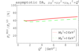
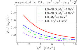
(a)	(b)

Figure 4: NLO calculation of twist-3 contribution to the proton form factor $F_{2}$ obtained for $M_{N}=0$ (5.6-5.7), using asymptotic DA (5.17) and $\mu_{R}^{2}=\mu_{F}^{2}=\mu_{R,1}^{2}=Q^{2}$: a) The ratio $F_{2}^{\rm NLO,fin}/F_{2}^{\rm LO}$ (i.e., the ratio of NLO correction to the LO prediction) evaluated for the default choice (6.1) $M_{B}^{2}=2$ GeV² (solid line), and for the test choice $M_{B}^{2}=1$ GeV² (dashed line). b) The twist-3 prediction to $F_{2}$ normalized to $\mu_{p}G_{D}$: NLO (thick solid line) and LO (thick dot-dashed line) for $M_{B}^{2}=2$ GeV², NLO (thin long dashed line) and LO (thin short dashed line) for $M_{B}^{2}=1$ GeV².

In Fig. 5 the change of scales $\mu_{R}^{2}$, $\mu_{F}^{2}$ and $\mu_{R,1}^{2}$ is investigated. As can be seen by comparing Figs. 4a and 5a, by taking $\mu_{F}^{2}=\mu_{R,1}^{2}=M_{B}^{2}$ and retaining $\mu_{R}^{2}=Q^{2}$, the ratio of NLO correction to the LO prediction is lowered to 69% - 44% for $1<Q^{2}<10$ GeV² and it decreases with $Q^{2}$. Thus, one can see that the $F^{\rm NLO,IR}_{2}$ and $F^{\rm NLO,UV}_{2}$ terms from Eq. (5.7) decrease the size of NLO correction. By changing $\mu_{R}^{2}$ to $M_{B}^{2}$ the ratio gets bigger since then there is no suppression due to the running of the $\alpha_{s}$. From Fig. 5b one can see that the change of scales does not influence much the value of the complete $F_{2}$ NLO prediction. In further calculation, if not specified differently, we, following [33], take $\mu_{R}^{2}=\mu_{F}^{2}=\mu_{R,1}^{2}=M_{B}^{2}$.

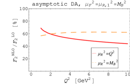
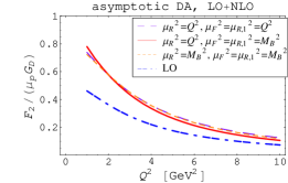
(a)	(b)

Figure 5: NLO calculation of twist-3 contribution to the proton form factor $F_{2}$ obtained for $M_{N}=0$ (5.6-5.7) and using asymptotic DA (5.17): a) The ratio $F_{2}^{\rm NLO}/F_{2}^{\rm LO}$ (i.e., the ratio of NLO correction calculated at to the LO prediction) calculated using $\mu_{F}^{2}=\mu_{R,1}^{2}=M_{B}^{2}$, while $\mu_{R}^{2}=Q^{2}$ (solid line), and $\mu_{R}^{2}=M_{B}^{2}$ (dashed line). b) The twist-3 prediction to $F_{2}$ normalized to $\mu_{p}G_{D}$: NLO for $\mu_{R}^{2}=Q^{2}$ and $\mu_{F}^{2}=\mu_{R,1}^{2}=Q^{2}$ (thin long dashed line), NLO for $\mu_{R}^{2}=Q^{2}$ and $\mu_{F}^{2}=\mu_{R,1}^{2}=M_{B}^{2}$ (thick solid line), NLO for $\mu_{R}^{2}=M_{B}^{2}$ and $\mu_{F}^{2}=\mu_{R,1}^{2}=M_{B}^{2}$ (thin short dashed line), and LO (thick dot-dashed line).

Finally, in Fig. 6 we investigate the size of the NLO correction and of the complete NLO prediction in dependence on the choice of DA (5.9). We employ the asymptotic (5.15) DA (solid line), BLW (5.14) DA (dash-dotted line), and the CZ-like DA (5.13) (dashed line). In Fig. 6b the LO predictions are denoted by thin lines and NLO predictions by thick lines. From Fig. 6a one can see that for $1<Q^{2}<10$ GeV² the ratio of NLO corrections to LO predictions amounts to 57% - 62% for the asymptotic DA, 61% - 76% for the BLW DA, and 66% - 86% for the CZ-like DA. Both LO predictions and NLO corrections are larger for the two DAs whose form differ from the asymptotic one.

In conclusion, we state that the NLO corrections to $F_{2}$ calculated at twist-3 taking $M_{N}=0$ are large, with $F_{2}^{\rm NLO}/F_{2}^{\rm LO}$ amounting to cca $60\%$, but varying for different DAs and depending on the choice of renormalization and factorization scales. The sensitivity of both LO and NLO corrections on the choice of $M_{B}$ is large and in the following we take the value (6.1) from Ref [28]. In contrast to the dependence of $F_{2}^{\rm NLO}/F_{2}^{\rm LO}$, the dependence of the complete NLO prediction of $F_{2}$ on the choice of renormalization and factorization scales is small and, if not stated otherwise, we take in the following $\mu_{R}^{2}=\mu_{F}^{2}=\mu_{R,1}^{2}=M_{B}^{2}$. The results for different DAs differ significantly.

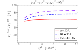
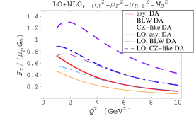
(a)	(b)

Figure 6: NLO calculation of twist-3 contribution to the proton form factor $F_{2}$ obtained for $M_{N}=0$ (5.6-5.7) using $\mu_{R}^{2}=\mu_{F}^{2}=\mu_{R,1}^{2}=M_{B}^{2}$. The displayed results correspond to asymptotic DAs (solid line), BLW DAs (dash-dotted line), and CZ-like DAs (dashed line). a) The ratio $F_{2}^{\rm NLO}/F_{2}^{\rm LO}$, i.e., the ratio of the NLO correction to the LO prediction. b) The twist-3 prediction to $F_{2}$ normalized to $\mu_{p}G_{D}$. Thick lines: NLO prediction. Thin lines: LO prediction.

6.2 Various contributions to $F_{1}$ and $F_{2}$

In preceding section we have discussed the size of the NLO corrections to $F_{2}$ calculated at twist-3 and taking $M_{N}=0$, and we have compared it to the corresponding LO predictions. In this section we want to analyze how large are these corrections in comparison to other contributions: mass effects, higher-twists and $x^{2}$ corrections calculated at LO. These effects are calculated on the basis of App. E, and Ref. [28].

6.2.1 $F_{2}$

The effect of including $M_{N}^{2}$ terms in LO twist-3 contribution to $F_{2}$ corresponds to the change of the LO contribution obtained using the asymptotic DA for $(-3)$-$23$ % when $1\leq Q^{2}\leq 10$ GeV². The change increases with $Q^{2}$ and one obtains similar numbers for all three DAs.

Let us now discuss higher-twist effects starting with twist-4. We note that for $M_{N}^{2}=0$ the twist-4 contribution to $F_{2}$ is 0 (the whole contribution (E.11), (E.12) is proportional to $M_{N}^{2}$). The ratio of LO twist-4 and twist-3 contributions to $F_{2}$ is in the range (-5) to (-35) % for asymptotic DAs, 2 to (-0.7) % for BLW DAs, and 13 to 24% for CZ-like DAs, when $1\leq Q^{2}\leq 10$ GeV². This behaviour is obviously very different for different DAs. In the case of the asymptotic DAs and the CZ-like DAs the absolute value of the ratio grows with $Q^{2}$, while for BLW the ratio decreases, changes sign and then absolute value increases. The role of the LO twist-4 contributions is thus small in the case of the results obtained using the BLW DAs, and more pronounced in the case of the other two investigated DAs (the BLW results seem to fall in some kind of minima). We have noticed the large sensitivity of these results on the choice of the parameters $f_{1}^{d}$ and $A_{1}^{u}$.

Finally, we summarize our findings about the size of various contributions to $F_{2}$ in Tables 6 and 7. One can see that twist-3 contributions are dominant and positive. The $x^{2}$-contributions are negative and the ratio of $x^{2}$-contributions and LO twist-3 contributions does not change much for various DAs. The twist-5 contributions are more pronounced than twist-4 contributions and for both the ratio to twist-3 contribution is very sensitive to the shape of DAs. The twist-3 NLO corrections are positive and cca 60%.

Hence, the twist-3 NLO corrections are indeed sizable and important.

Table 6: The size of various contributions to the proton form factor $F_{2}$ (normalized to LO twist-3 contribution calculated for $M_{N}^{2}\neq 0$) in the range $1\leq Q^{2}\leq 10$ GeV².

DAs	$\displaystyle\frac{F_{2}^{\rm LO,tw-3}|_{M_{N}^{2}=0}}{F_{2}^{\rm LO,tw-3}}$	$\displaystyle\frac{F_{2}^{\rm LO,tw-4}}{F_{2}^{\rm LO,tw-3}}$	$\displaystyle\frac{F_{2}^{\rm LO,tw-5}}{F_{2}^{\rm LO,tw-3}}$	$\displaystyle\frac{F_{2}^{{\rm LO},x^{2}-{corr.}}}{F_{2}^{\rm LO,tw-3}}$
asy.	103 - 81%	(-5) - (-35)%	34 - 91%	(-35) - (-43)%
BLW	98 - 81%	2 - (-0.7)%	14 - 21%	(-33) - (-28)%
CZ-like	92 - 81%	13 - 24 %	(-13) - (-29)%	(-31) - (-18)%

Table 7: The size of NLO twist-3 corrections to the proton form factor $F_{2}$ (normalized to LO twist-3 contribution calculated for $M_{N}^{2}\neq 0$) in the range $1\leq Q^{2}\leq 10$ GeV² and for three choices of scales: a) $\mu_{R}^{2}=\mu_{F}^{2}=\mu_{R,1}^{2}=Q^{2}$, b) $\mu_{R}^{2}=Q^{2},\mu_{F}^{2}=\mu_{R,1}^{2}=M_{B}^{2}$, c) $\mu_{R}^{2}=\mu_{F}^{2}=\mu_{R,1}^{2}=M_{B}^{2}$.

DAs	$\displaystyle\frac{F_{2}^{\rm NLO,tw-3}|_{M_{N}^{2}=0,a)}}{F_{2}^{\rm LO,tw-3}}$	$\displaystyle\frac{F_{2}^{\rm NLO,tw-3}|_{M_{N}^{2}=0,b)}}{F_{2}^{\rm LO,tw-3}}$	$\displaystyle\frac{F_{2}^{\rm NLO,tw-3}|_{M_{N}^{2}=0,c)}}{F_{2}^{\rm LO,tw-3}}$
asy.	62 - 57%	71 - 36%	58 - 51%
BLW	62 - 68%	72 - 44%	59 - 62%
CZ-like	63 - 76%	74 - 49%	61 - 69%

6.2.2 $F_{1}$

In the next section we will proceed to the comparison of our results to the experimental data and for that we need the $F_{1}$ contribution as well (we have at our disposal the experimental data for $G_{M}$ and $G_{E}$). Here we thus analyze the LO contributions to $F_{1}$.

The effect of including $M_{N}^{2}$ terms in LO twist-3 contribution to $F_{1}$ corresponds to the change of the LO contribution obtained using the asymptotic DA for $6$-$24$ % when $1\leq Q^{2}\leq 10$ GeV². The change decreases and then increases with $Q^{2}$ (minimum at $Q^{2}\approx 2$ GeV² and one obtains similar numbers for all three DAs. But in the case of $F_{1}$, twist-3 contribution is negative and small in comparison with twist-4 contribution.

In contrast to $F_{2}$, twist-4 contribution to $F_{1}$ is not proportional to $M_{N}^{2}$ (see App. E). The effect of including $M_{N}^{2}$ terms in LO twist-4 to $F_{2}$ corresponds to the change of the contribution obtained using the asymptotic DAs for $12$-$30$ % when $1\leq Q^{2}\leq 10$ GeV². The numbers are similar for both asymptotic and BLW DAs, but smaller and negative for CZ-like DAs. The ratio of twist-3 and twist-4 LO contributions to $F_{1}$ is (-19)-(-7)% for the asymptotic DAs, (-25)-(-12)% for the BLW DAs, and (-46)-(-105)% for the CZ-like DAs. Hence, apart from the results for CZ-like DAs at higher $Q^{2}$, the twist-4 contributions is larger than the twist-3 contribution.

Finally, to summarize our findings about the size of various contributions to $F_{1}$ in Table 8, we state that the twist-4 contributions are dominant and positive.

Table 8: The size of various contributions to the proton form factor $F_{1}$ (normalized to LO twist-4 contribution calculated for $M_{N}^{2}\neq 0$) in the range $1\leq Q^{2}\leq 10$ GeV².

DAs	$\displaystyle\frac{F_{1}^{\rm LO,tw-3}}{F_{1}^{\rm LO,tw-4}}$	$\displaystyle\frac{F_{1}^{\rm LO,tw-5}}{F_{1}^{\rm LO,tw-4}}$	$\displaystyle\frac{F_{1}^{\rm LO,tw-6}}{F_{1}^{\rm LO,tw-4}}$	$\displaystyle\frac{F_{1}^{{\rm LO},x^{2}-{corr.}}}{F_{1}^{\rm LO,tw-4}}$
asy.	(-19) - (-7)%	(-4) - (-5)%	3 - 2%	5 - 2%
BLW	(-25) - (-12)%	(-2)%	3 - 2%	6 - 3%
CZ-like	(-46) - (-105)%	5 - 37%	5 - 14%	10 - 22%

6.3 Comparison to experimental data

Finally, let us compare our findings to experimental data.

In Figs. 7, 8 and 9 we display the results for $G_{M}/(\mu_{p}G_{D})$, $\mu_{p}G_{E}/G_{M}$ and $\sqrt{Q^{2}}F_{2}/(\kappa_{p}F_{1})$ obtained using the asymptotic DAs (solid line), the BLW DAs (dash-dotted line), and the CZ-like DAs (dashed line). The DA parameters are given in Sec. 5.2.

For comparison, in Figs. 7a, 8a and 9a we present the LO predictions obtained on the basis of the results from Ref. [28], where the higher-twist contributions (up to twist-6) and $x^{2}$ correction were included and the value of $\lambda_{1}$ (6.2) was used. The NLO predictions, i.e. the LO predictions obtained on the basis of the results from Ref. [28] plus NLO corrections for twist-3 ($M_{N}=0$ case) calculated in this work (with $s_{0}$ and $M_{B}$ as from Eq. (6.1), while $\mu_{R}^{2}=\mu_{F}^{2}=\mu_{R,1}^{2}=M_{B}^{2}$), are displayed in Figs. 7b, 8b and 9b. Here we investigate also the change of the results with the choice of $\lambda_{1}$. The NLO results obtained using the default value of $\lambda_{1}$ (6.2) are, as in Fig. 7a, 8a and 9a, denoted by thin lines, while thick lines denote the NLO results obtained employing the corrected value of $\lambda_{1}$ (6.3).

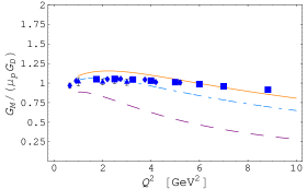
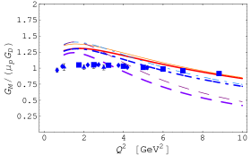
(a)	(b)

Figure 7: LCSR prediction for the proton form factor $G_{M}$ normalized to $\mu_{p}G_{D}$. The displayed results correspond to asymptotic DAs (solid line), BLW DAs (dash-dotted line), and CZ-like DAs (dashed line) – see Sec. 5.2 for the DA parameters. a) LO prediction on the basis of the results from Ref. [28] (i.e., the higher-twist contributions (up to twist-6) and $x^{2}$ correction included). b) LO prediction on the basis of the results from Ref. [28] plus NLO correction for twist-3 ($M_{N}=0$ case) calculated in this work (choice of scales as in Fig. 6). Thin lines: the default value of $\lambda_{1}$ (6.2). Thick lines: the corrected value of $\lambda_{1}$ (6.3). Experimental data obtained using Rosenbluth separation: $\blacktriangle$ SLAC 1994 [61], $\blacksquare$ SLAC 1994 [62], $\blacklozenge$ JLab 2004 [63], $\bigstar$ JLab 2005 [64].

In Fig. 7 we display the LCSR prediction for $G_{M}$ normalized to $\mu_{p}G_{D}$. The displayed experimental data were obtained using Rosenbluth separation: $\blacktriangle$ SLAC 1994 [61], $\blacksquare$ SLAC 1994 [62], $\blacklozenge$ JLab 2004 [63], $\bigstar$ JLab 2005 [64]. The LO results 7a favour the asymptotic and BLW DAs. The inclusion of NLO corrections (compare thin lines in Figs. 7a and 7b) raises the predictions. The change of $\lambda_{1}$ to the corrected value (6.3) lowers the NLO results (thick lines) slightly. The NLO results seem to overshoot the data at lower $Q^{2}$, while at higher $Q^{2}$ again the asymptotic and BLW results seem to be closer to the data than the results obtained using the CZ-like DAs.

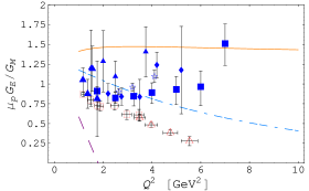
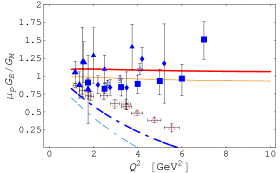
(a)	(b)

Figure 8: LCSR prediction for the proton form factors ratio $\mu_{p}G_{E}/G_{M}$. The displayed results correspond to asymptotic DAs (solid line), and BLW DAs (dash-dotted line) – see Sec. 5.2 for the DA parameters. a) LO prediction on the basis of the results from Ref. [28] (i.e., the higher-twist contributions up to twist-6 and $x^{2}$ correction included). b) LO prediction on the basis of the results from Ref. [28] plus NLO correction (to $F_{2}$) for twist-3 ($M_{N}=0$ case) calculated in this work (choice of scales as in Fig. 6). Thin lines: the default value of $\lambda_{1}$ (6.2). Thick lines: the corrected value of $\lambda_{1}$ (6.3). Experimental data obtained using Rosenbluth separation: $\blacksquare$ SLAC 1994 [62], $\blacklozenge$ JLab 2004 [63], $\bigstar$ JLab 2005 [64], $\blacktriangle$ SLAC 1970 (small) [65] and Bonn 1971 (big) [66] data revised in [67]. Experimental data obtained via polarization transfer: $\triangle$ JLab 2001 [68], $\Box$ JLab 1999 [69].

In Fig. 8 we present the LCSR prediction for $\mu_{p}G_{E}/G_{M}$. We use the experimental data obtained using Rosenbluth separation ( $\blacksquare$ SLAC 1994 [62], $\blacklozenge$ JLab 2004 [63], $\bigstar$ JLab 2005 [64], $\blacktriangle$ SLAC 1970 (small) [65] and Bonn 1971 (big) [66] data revised in [67]) as well as more reliable experimental data obtained via polarization transfer ($\triangle$ JLab 2001 [68], $\Box$ JLab 1999 [69]). The LO results displayed in Fig. 8a show that while the results obtained using the CZ-like DAs are quite low and well beyond the data, and the results obtained the asymptotic DAs are on the high edge of the data, the BLW results seem to be in better agreement with the data, but one cannot really make some conclusive statements. The inclusion of NLO corrections (compare thin lines in Figs. 8a and 8b) lowers the predictions significantly, while the change of $\lambda_{1}$ to the corrected value (6.3) raises the NLO results (thick lines) slightly. Note that the results obtained using the CZ-like DAs are ruled out and left out. One can see now the NLO results, especially the results obtained using the corrected value for $\lambda_{1}$, are in quite good agreement with the data. The results obtained using the asymptotic DAs seem to describe well the experimental data obtained using the Rosenbluth separation, while the NLO results obtained using the BLW DAs seem to follow the slope of the preferred experimental data obtained via polarization transfer.

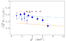
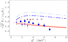
(a)	(b)

Figure 9: LCSR prediction for the proton form factors ratio $\sqrt{Q^{2}}F_{2}/(\kappa_{p}F_{1})$. The displayed results correspond to asymptotic DAs (solid line), and BLW DAs (dash-dotted line) – see Sec. 5.2 for the DA parameters. a) LO prediction on the basis of the results from Ref. [28] (i.e., the higher-twist contributions up to twist-6 and $x^{2}$ correction included). b) LO prediction on the basis of the results from Ref. [28] plus NLO correction (to $F_{2}$) for twist-3 ($M_{N}=0$ case) calculated in this work (choice of scales as in Fig. 6). Thin lines: the default value of $\lambda_{1}$ (6.2). Thick lines: the corrected value of $\lambda_{1}$ (6.3). Experimental data obtained using Rosenbluth separation: $\blacksquare$ SLAC 1994 [62], $\blacktriangle$ SLAC 1994 [61]. Experimental data obtained via polarization transfer: $\triangle$ and $\Box$ as in Ref. [28], Fig. 15 (M. Jones, private communication).

In Fig. 9 we present the LCSR prediction for $\sqrt{Q^{2}}F_{2}/(\kappa_{p}F_{1})$. We display the experimental data obtained using Rosenbluth separation ($\blacksquare$ SLAC 1994 [62], $\blacktriangle$ SLAC 1994 [61]) and preferred experimental data obtained via polarization transfer ($\triangle$ and $\Box$ as in Ref. [28], Fig. 15 (M. Jones, private communication)). The LO results are displayed in Fig. 9a and while the results obtained using the asymptotic DAs are on the lower edge of the data, the BLW results seem to fall close to the data (at least for lower $Q^{2}$). The inclusion of NLO corrections (compare thin lines in Figs. 9a and 9b) raises the predictions significantly, while the change of $\lambda_{1}$ to the corrected value (6.3) lowers the NLO results (thick lines) slightly. As in the case of the $\mu G_{E}/G_{M}$ results displayed in Fig. 8, one can see that the NLO results, especially the results obtained using the corrected value for $\lambda_{1}$, are in good agreement with the data. Again, the results obtained using the asymptotic DAs seem to describe well the experimental data obtained using the Rosenbluth separation, while the NLO results obtained using the BLW DAs seem to follow the slope of the experimental data obtained via polarization transfer.

In conclusion, the inclusion of NLO corrections calculated at twist-3 for $M_{N}=0$ introduces significant changes in the LCSR predictions for $G_{M}/(\mu_{p}G_{D})$, $\mu_{p}G_{E}/G_{M}$ and $\sqrt{Q^{2}}F_{2}/(\kappa_{p}F_{1})$. It seems that NLO corrections, as well as the use of the corrected value for $\lambda_{1}$ (6.3), bring the predictions for $\mu_{p}G_{E}/G_{M}$ and $\sqrt{Q^{2}}F_{2}/(\kappa_{p}F_{1})$ in better agreement with the experimental data. For these quantities, the results obtained using the asymptotic DAs seem to describe well the experimental data obtained using the Rosenbluth separation, while the NLO results obtained using the BLW DAs seem to follow the slope of the experimental data obtained via polarization transfer.

7 Summary and conclusions

In this work the first attempt has been made to asses the size of NLO corrections to nucleon form factors.

In LCSR approach dealing with nucleons is much more demanding than dealing with mesons, even at LO. For one, the number of contributing terms is rather large, the expressions are more involved, and the presence of three, instead of two, partons with corresponding momenta makes the calculation more complicated. All this is present at NLO also, with additional difficulties of one-loop calculation and larger number of contributing Feynman diagrams.

In order to calculate the NLO corrections, we have started with the simple $M_{N}^{2}=0$ (but $M_{N}\neq 0$) approximation, i.e., the approximation corresponding to the first two terms in the expansion in nucleon mass (2.44). In that approximation only the leading twist, twist-3, and next-to-leading twist, twist-4, contributions appear. But to our surprise it turned out that the collinear divergences appearing in one-loop calculation do not cancel on the level of separate twist and that actually mixing appears which, without knowing the corresponding kernels, disables us in determing the finite contributions (see Sec. 4.4).

Hence, we have strengthen our approximation and considered $M_{N}=0$ approximation (corresponds to the first term in (2.44)) in which only twist-3 contributes and the evolution kernels are known. We have shown the explicit cancellation of collinear, as well as, UV singularities (see Sec. 4.3). The finite twist-3 NLO contributions to the correlation function are thus obtained in $M_{N}=0$ approximation and relevant invariant functions are listed in App. C.

We note that the observation of mixing of twist-3 and twist-4 NLO contributions is in nature similar to the observation given in Sec. 3.4 that the gauge invariant results are obtained not twist-by-twist but order-by-order in $M_{N}$. The gauge condition is for $M_{N}=0$ case satisfied both in LO and NLO order. For $M_{N}^{2}=0$ and $M_{N}\neq 0$ we have shown to LO that gauge condition is satisfied only when the sum of all contributing terms is taken into account, i.e., both twist-3 and twist-4 contributions. The additional condition is that the asymptotic forms of twist-3 DAs are used (no conditions, at least at this order, on twist-4 DAs). Hence, gauge invariance can be satisfied order by order in the expansion in $M_{N}$ (2.44) with possibly some additional conditions on the form of DAs.

To repeat, by switching-on the nucleon mass, which is, of course necessary in order to determine higher-twists, we are at $M_{N}^{2}=0$ and $M_{N}\neq 0$ stuck with mixing of the contributions corresponding to different twists. This ”mixing” can be seen even at LO through the check of gauge invariance with respect to photon. If we take $M_{N}^{2}\neq 0$, there are no collinear divergences whose cancellation we should take care of and no apparent ”mixing”. But the NLO expressions are more involved and there are additional open problems one should solve before attacking higher-order higher-twist calculations. For example, there is an open technical problem elaborated in Sec. 4.4 and connected to the calculation of the NLO contributions to second and third case defined in (2.28). The calculation of NLO corrections for $M_{N}\neq 0$ case and thus NLO corrections to higher twists we postpone for some other time.

In Sec. 6 we have presented and analyzed our numerical results based on the calculation of NLO corrections in $M_{N}=0$ approximation, i.e., twist-3 NLO corrections in that approximation. Using Ioffe current in this approximation we are able to calculate only the corrections to $F_{2}$ nucleon form factor. To make a full analysis and estimate the importance of NLO corrections, we have also included the LO results obtained beyond this approximation, i.e., leading twist and higher-twist results obtained in Ref. [28]. We have considered here just the proton case.

For $F_{1}$ twist-4 LO contributions are dominant and positive, and there are no NLO corrections in $M_{N}=0$ approximation. When one considers the size of various contributions to $F_{2}$, one realizes that twist-3 LO contributions are dominant and positive. The twist-5 LO contributions are more pronounced than twist-4 LO contributions and for both the ratio to twist-3 LO contribution is very sensitive to the shape of DAs. The $x^{2}$-contributions are negative and the ratio of $x^{2}$-contributions and LO twist-3 contributions does not change much for various DAs. The twist-3 NLO corrections are positive and cca 60%. The NLO corrections to $F_{2}$ calculated at twist-3 taking $M_{N}=0$ are thus large. They vary for different DAs and depend on the choice of renormalization and factorization scales. In contrast to the dependence of $F_{2}^{\rm NLO}/F_{2}^{\rm LO}$, the dependence of the complete NLO prediction of $F_{2}$ on the choice of renormalization and factorization scales is small.

The inclusion of NLO corrections calculated at twist-3 for $M_{N}=0$ introduces significant changes in the LCSR predictions for $G_{M}/(\mu_{p}G_{D})$, $\mu_{p}G_{E}/G_{M}$ and $\sqrt{Q^{2}}F_{2}/(\kappa_{p}F_{1})$. It seems that NLO corrections, as well as the use of the corrected value for $\lambda_{1}$ (6.3), bring the predictions for $\mu_{p}G_{E}/G_{M}$ and $\sqrt{Q^{2}}F_{2}/(\kappa_{p}F_{1})$ in better agreement with the experimental data. For these quantities, the results obtained using the asymptotic DAs seem to describe well the experimental data obtained using the Rosenbluth separation, while the NLO results obtained using the BLW DAs seem to follow the slope of the preferred experimental data obtained via polarization transfer.

Further analysis and inclusion of NLO corrections at higher-twists is needed to draw some more conclusive results.

Acknowledgements

We are indebted to V. Braun for both proposing this subject and for clarifying discussions. K. P-K. would like to thank the theory group at the University of Regensburg for its warm hospitality and would also like to thank G. Duplančić, K. Kumerički, A. Lenz, B. Melić, D. Müller, and A. Peters, for taking the time to discuss some aspects of this work. This project has been supported by the German Research Foundation (DFG) under the contract no. 9209070, Croatian Ministry of Science, Education and Sport under the contract no. 098-0982930-2864 and the Studienstiftung des deutschen Volkes.

Appendix A Feynman rules

In calculating $(-i\,T_{\mu})$ where $T_{\mu}$ is a correlator function (2.5) we use the standard Feynman rules for quark and gluon propagators and vertices, as well as for the quark-photon vertex. For loop integrals one has to introduce the usual integration over loop momenta.

The vertex corresponding to the interpolating nucleon current given by (2.8) reads

$$\mbox{u-quark(}\alpha,a\mbox{)--u-quark(}\beta,b\mbox{)--d-quark(}\gamma,c\mbox{)-- Ioffe current}:\;\left(C\gamma_{\lambda}\right)_{\alpha\beta}\;\left(\gamma_{5}\gamma^{\lambda}\right)_{\delta\gamma}\;\varepsilon^{abc}\,,$$ (A.1)

where all quark lines are going in the vertex and the order of u,u, and d-quarks with corresponding Lorentz ($\alpha,\beta,\gamma$) and colour ($a,b,c$) indices is counterclockwise. Furthermore, $(C\gamma_{\lambda})^{T}=C\gamma_{\lambda}$, i.e., $\left(C\gamma_{\lambda}\right)_{\alpha\beta}=\left(C\gamma_{\lambda}\right)_{\beta\alpha}$.

The (incoming) nucleon “projector” corresponding to (2.11) and the first case of (2.28) is given by

$$\mbox{u-quark(}u_{1}P,\alpha,a\mbox{)--u-quark(}u_{2}P,\beta,b\mbox{)--d-quark(}u_{3}P,\gamma,c\mbox{):}$$ (A.2)

$$\hskip 56.9055pt\qquad\;\frac{1}{4}\;\int{\cal D}u\,F^{(i)}(u_{1},u_{2},u_{3})\;\;X^{(i)}_{\alpha\beta}\;Y^{(i)}_{\gamma}\;\frac{\varepsilon^{abc}}{6}\,,$$

where all quark lines are outgoing from the nucleon blob and the order is clockwise. The trivial identity $X^{(i)}_{\alpha\beta}=\left(X^{(i)}\right)^{T}_{\beta\alpha}$ together with (2.12) is useful in some cases.

The typical contribution obtained using the general Lorentz decomposition (2.11) and Ioffe current (2.8), i.e., Feynman rules (A.2) and (A.1), respectively, has two parts. For the $d-d$ quark line, by going, following the standard rule, in the opposite direction of the fermion line, one obtains the product of $\gamma$ matrices with the nucleon spinor. The $u-u$ lines close the trace and obviously, in writing it down, one goes opposite to the direction of the one quark line and along the other one. The latter case corresponds to $\left(\gamma_{\mu 1}\gamma_{\mu 2}\ldots\gamma_{\mu_{n}}\right)^{T}$ (where $\gamma_{\mu 1}\ldots\gamma_{\mu_{n}}$ is the order of $\gamma$ matrices opposite to the direction of the fermion line) and one then makes use of

$$\left(\gamma_{\mu 1}\gamma_{\mu 2}\ldots\gamma_{\mu_{n}}\right)^{T}=(-1)^{n}C\gamma_{\mu n}\ldots\gamma_{\mu_{1}}C^{-1}\,,$$ (A.3)

i.e. when going in the direction of fermion line one puts the $\gamma$ matrices on the that line between $C$ and $C^{-1}$.

Finally, let us mention that the usual relations for SU($N_{C}$) algebra should be employed in calculating the colour factors. Since we are dealing here with nucleon described by three quarks we are actually already assuming $N_{C}=3$ and only this choice leads to gauge invariant results. Obviously,

$$\varepsilon^{abc}\;\varepsilon^{abc}=6\,.$$ (A.4)

Appendix B $\gamma_{5}$ ambiguity in dimensional regularization

When using dimensional regularization, one runs into trouble with quantities that have the well-defined properties only in $D=4$ space-time dimensions, that is, with the Levi-Civita tensor $\epsilon_{\mu\nu\lambda\kappa}$, which is a genuine 4 dimensional object, and consequently with the pseudoscalar $\gamma_{5}$ Dirac matrix. Let us mention that the appearance and mixing with evanescent operators [70], as well as, the definition of Fierz transformation in $D$ dimensions are also connected to this problem. We shall handle it similarly to Ref. [52] with some additional finesse concerning Chisholm identity (see Sec. 4.2). Below we explain the general features of the ambiguities that we encounter in our calculation. In order to resolve these one should generally use some other input like the knowledge of the quantity that does not suffer from ambiguities, condition of cancellation of singularities, condition of preservation of gauge invariance, Ward identities etc.

B.1 General remarks – trace ambiguity

The generalization of the $\gamma_{5}$ matrix in $D$ dimensions represents a problem, since it is not possible to simultaneously retain its anticommuting and trace properties. In practice, the ambiguity arises when evaluating a trace containing a $\gamma_{5}$ and pairs of contracted $\gamma$ matrices and/or pairs of Dirac slashed loop momenta . To deal with a $\gamma_{5}$ matrix, several possible schemes have been proposed in the literature.

In the so-called naive-$\gamma_{5}$ scheme [54], the anticommutation property of $\gamma_{5}$ is retained, while the cyclicity of the trace is abandoned. The traces obtained by cyclic permutation of the matrices differ by $D-4$. Consequently, if the trace is multiplied by a pole in $D-4$, there appears a finite ambiguity in the result. An alternative scheme has been proposed in the original paper on the dimensional regularization by ’t Hooft and Veltman [55], and further systematized by Breitenlohner and Maison [56]. In this scheme, to which we refer as HV scheme, the anticommutativity of $\gamma_{5}$ is abandoned. In contrast to naive-$\gamma_{5}$ scheme, this scheme is claimed to be mathematically consistent but still not without drawbacks. Namely, this prescription for $\gamma_{5}$ violates the Ward identities and introduces “spurious” anomalies which violate chiral symmetry. To restore the Ward identities, finite counterterms should be added order by order in perturbation theory [71]. In this scheme, the cyclicity of the trace is retained.

If a trace contains an even number of $\gamma_{5}$ matrices, then the property $\gamma_{5}^{2}=1$ can be used to eliminate $\gamma_{5}$’s from the trace, and the Ward identities are preserved if the naive-$\gamma_{5}$ scheme is used [54] (the cyclicity of the trace is restored and the corresponding results are unambiguous). On the other hand, in the HV scheme the “spurious” anomalies can occur owing to the non-anticommuting property of $\gamma_{5}$. As for the traces containing an odd number of $\gamma_{5}$ matrices, we are left with the above mentioned ambiguities in the results.

For details, we refer to App. A in Ref. [52].

B.2 General remarks – Chisholm identity

Additionally, the Chisholm identity that we need in our calculation

$$\gamma^{\mu}\varepsilon_{\mu\alpha\beta\gamma}=i\left(\gamma_{\alpha}\gamma_{\beta}\gamma_{\gamma}-g_{\alpha\beta}\gamma_{\gamma}+g_{\gamma\alpha}\gamma_{\beta}-g_{\beta\gamma}\gamma_{\alpha}\right)$$ (B.1)

is strictly speaking valid only in $D=4$ dimensions. The modification for HV scheme can be found in the literature (see, for example, Tracer [72] manual) but we have not been able to find any recipe for the naive-$\gamma_{5}$ scheme.

Our analysis of the problem has shown that when applying the Chisholm identity on expressions of the form

$$\gamma^{\mu}\gamma_{\kappa}\gamma^{\nu}\varepsilon_{\mu\nu\alpha\beta}$$ (B.2)

different results appear in dependence of whether one first contracts the Levi-Civita tensor with the $\gamma$ matrix on the left or the right side of the non-contracted matrix ($\gamma_{\kappa}$ in this case). The difference is again, as expected, proportional to $D-4$. For example,

$$\gamma^{\mu}\gamma^{\alpha}\gamma_{\kappa}\gamma^{\nu}\gamma^{\beta}\varepsilon_{\mu\nu\alpha\beta}$$ (B.3a)

has two sets of results

$$\left(\gamma^{\mu}\varepsilon_{\mu\nu\alpha\beta}\right)\gamma^{\alpha}\gamma_{\kappa}\gamma^{\nu}\gamma^{\beta}=\gamma^{\mu}\left(\gamma^{\alpha}\varepsilon_{\mu\nu\alpha\beta}\right)\gamma_{\kappa}\gamma^{\nu}\gamma^{\beta}=-i(D-4)(D-2)(D-1)\gamma_{\kappa}\gamma_{5}\,,$$ (B.3b)

while

$$\gamma^{\mu}\gamma^{\alpha}\gamma_{\kappa}\left(\gamma^{\nu}\varepsilon_{\mu\nu\alpha\beta}\right)\gamma^{\beta}=\gamma^{\mu}\gamma^{\alpha}\gamma_{\kappa}\gamma^{\nu}\left(\gamma^{\beta}\varepsilon_{\mu\nu\alpha\beta}\right)=i(D-4)(D-2)(D-1)\gamma_{\kappa}\gamma_{5}\,.$$ (B.3c)

So, when using the Chisholm identity in its form as in $D=4$ dimensions (which should be in agreement with the “philosophy“ of naive-$\gamma_{5}$ scheme) we again, as in the case of trace ambiguity, encounter the ambiguity proportional to $D-4$, which, when multiplied by pole in $D-4$, possibly leads to finite ambiguity of the results.

Appendix C NLO results for $M_{N}=0$ case

C.1 Formalism and notation

In $M_{N}=0$ case we cannot asses the ${\cal A}$ contribution from Eq. (2.34), while the corresponding ${\cal B}$ contribution we list in this section.

The ${\cal B}$ function can be written as a convolution in terms of $V_{1}$ and $A_{1}$ nucleon DAs

$${\mathcal{B}}_{M_{N}=0}(Q^{2},P^{\prime 2})$$ (C.1)

$$= T_{\mathcal{B},V_{1},M_{N}=0}(\{x_{k}\},Q^{2},P^{\prime 2};\mu_{F}^{2})\;\otimes\;V_{1}(\{x_{k}\};\mu_{F}^{2})$$

$$+T_{\mathcal{B},A_{1},M_{N}=0}(\{x_{k}\},Q^{2},P^{\prime 2};\mu_{F}^{2})\otimes\;A_{1}(\{x_{k}\},\mu_{F}^{2})\,,$$

or in terms of twist-3 nucleon DA $\Phi_{3}=V_{1}-A_{1}$

$${\mathcal{B}}_{M_{N}=0}(Q^{2},P^{\prime 2})$$ (C.2)

$$= T_{\mathcal{B},\Phi,M_{N}=0}(\{x_{k}\},Q^{2},P^{\prime 2};\mu_{F}^{2})\;\otimes\;\Phi_{3}(\{x_{k}\};\mu_{F}^{2})\,.$$

Here $q=-Q^{2}$ is a photon virtuality and $P^{\prime}=P-q$, while $P$ is incoming nucleon momentum. The factorization scale is denoted by $\mu_{F}^{2}$, and by $\{x_{k}\}$ the quark momentum fractions $x_{1}$, $x_{2}$ and $x_{3}$ are denoted. Note that $x_{1}$ and $x_{2}$ denote the momentum fractions of $u$-quarks, while $x_{3}$ correspond to the momentum fraction of the $d$-quark. A stated in Eq. (2.25), $V_{1}$ is symmetric and $A_{1}$ antisymmetric under $x_{1}\leftrightarrow x_{2}$ exchange.

It is convenient to introduce a dimensionless quantity

$$W=\frac{P^{\prime 2}+Q^{2}}{Q^{2}}\,,$$ (C.3)

and we will from now on express the ${\cal B}$ function using $W$ instead of $P^{\prime 2}$.

Generally, we write

$${\cal B}_{M_{N}=0}(Q^{2},W)=\frac{1}{Q^{2}}\,\sum_{i}\,T_{{\cal B},F^{(i)},M_{N}=0}(\{x_{k}\},W;\mu_{F}^{2}/Q^{2})\otimes F^{(i)}(\{x_{k}\};\mu_{F}^{2})$$ (C.4)

with $F^{(i)}$ denoting nucleon DAs and $T_{{\cal B},F^{(i)},M_{N}=0}$ the corresponding ”hard-scattering” part. The nucleon DAs are intrinsically non-perturbative quantities but their evolution to scale $\mu_{F}^{2}$ can be calculated perturbatively. Nevertheless, we take into account only the LO evolution or neglect the evolution completely. The ”hard-scattering” part is calculated perturbatively and in this work the calculation to NLO is performed. Hence, following Sec.4.3 (see Eqs. (4.29) and (4.31), and Eqs. (LABEL:eq:finiteM-V1A1) and (LABEL:eq:FiniteM-V1A1-NLO) ) we can write the expansion of $T_{{\cal B},F^{(i)},M_{N}=0}$ as

$$T_{{\cal B},F^{(i)},M_{N}=0}(\{x_{k}\},W;\mu_{F}^{2}/Q^{2})$$

$$= \left\{T_{{\cal B},F^{(i)},M_{N}=0}^{\rm LO}(\{x_{k}\},W)+\frac{\alpha_{s}(\mu_{R}^{2})}{4\pi}T_{{\cal B},F^{(i)},M_{N}=0}^{\rm NLO}(\{x_{k}\},W;\mu_{F}^{2}/Q^{2},\mu_{R,1}^{2}/Q^{2})+\cdots\right\}\,,$$

where

$$T_{{\cal B},F^{(i)},M_{N}=0}^{\rm NLO}(\{x_{k}\},W;\mu_{F}^{2}/Q^{2},\mu_{R,1}^{2}/Q^{2})$$ (C.6)

$$= T_{{\cal B},F^{(i)},M_{N}=0}^{\rm NLO,fin}(\{x_{k}\},W)$$

$$+T_{{\cal B},F^{(i)},M_{N}=0}^{\rm NLO,UV}(\{x_{k}\},W)\;\ln(\mu_{R,1}^{2}/Q^{2})$$

$$+T_{{\cal B},F^{(i)},M_{N}=0}^{\rm NLO,IR}(\{x_{k}\},W)\;\ln(\mu_{F}^{2}/Q^{2})\,,$$

and $\mu_{R}^{2}$ and $\mu_{R,1}^{2}$ scales denote the coupling constant and Ioffe current renormalization scales (which are in practice often taken the same, and even same to the factorization scale $\mu_{F}^{2}$, but are in principle independent).

Note that all order result for $T_{{\cal B},F^{(i)},M_{N}=0}$ would not depend on the choice of the renormalization scale, but the truncation of the series to any finite order (in or case NLO) introduces the residual dependence. This dependence would be stabilized by inclusion of higher-orders ($\alpha_{s}^{n}$, $n\geq 2$). One is left also with the residual dependence of ${\cal B}$ on the factorization scale (see Ref. [73] for details on that point).

In the following we summarize the LO and NLO results for $T_{{\cal B},F^{(i)},M_{N}=0}$. These are proportional either to $e_{u}$ or $e_{d}$ being $u$ and $d$-quark charges (depending on where the photon coupled), respectively. Remember that we are displaying here the proton case, while for the neutron $e_{u}$ and $e_{d}$ have to be exchanged. Hence, we burden our notation with one more index

$$T_{{\cal B},F^{(i)},M_{N}=0}^{\cdots}(\cdots)=T_{{\cal B},F^{(i)},M_{N}=0}^{\cdots,e_{d}}(\cdots)+T_{{\cal B},F^{(i)},M_{N}=0}^{\cdots,e_{u}}(\cdots)\,.$$ (C.7)

In order to simplify the expressions and write them in a form most suitable for further calculation, we introduce the following functions

$$g_{0}(x_{i},W) = \frac{1}{(x_{i}W-1+i\eta)}\,,$$

$$g_{1}(x_{i},W) = -\frac{\ln(1-x_{i}W-i\eta)}{(1-x_{i}W-i\eta)}\,,$$

$$g_{2}(x_{i},W) = -\frac{\ln^{2}(1-x_{i}W-i\eta)}{(1-x_{i}W-i\eta)}\,,$$

$$g_{3}(x_{i},W) = \frac{\ln(1-x_{i}W-i\eta)}{(W+i\eta)}\,,$$

$$g_{4}(x_{i},W) = \frac{\ln(1-x_{i}W-i\eta)}{(W+i\eta)^{2}}\,,$$

$$g_{5}(x_{i},W) = \frac{\ln^{2}(1-x_{i}W-i\eta)}{(W+i\eta)}\,,$$

$$g_{6}(x_{i},W) = \frac{\ln^{2}(1-x_{i}W-i\eta)}{(W+i\eta)^{2}}\,,$$

$$g_{7}(x_{i},x_{j},W) = -\frac{\ln(1-(x_{i}+x_{j})W-i\eta)}{(1-x_{i}W-i\eta)}\,,$$

$$g_{8}(x_{i},x_{j},W) = -\frac{\ln^{2}(1-(x_{i}+x_{j})W-i\eta)}{(1-x_{i}W-i\eta)}\,,$$

$$g_{9}(x_{i},x_{j},W) = \frac{\ln(1-(x_{i}+x_{j})W-i\eta)}{(W+i\eta)}\,,$$

$$g_{10}(x_{i},x_{j},W) = \frac{\ln(1-(x_{i}+x_{j})W-i\eta)}{(W+i\eta)^{2}}\,,$$

$$g_{11}(x_{i},x_{j},W) = \frac{\ln^{2}(1-(x_{i}+x_{j})W-i\eta)}{(W+i\eta)}\,,$$

$$g_{12}(x_{i},x_{j},W) = \frac{\ln^{2}(1-(x_{i}+x_{j})W-i\eta)}{(W+i\eta)^{2}}\,.$$ (C.8)

Note that we have kept $i\eta$ terms ($\eta>0$ and $\eta\ll$) coming from the Feynman diagram calculation (quark and gluon propagators), which will enable the correct determination of imaginary parts necessary for LCSR in Sec. 5.

C.2 Complete list of results

In previously introduced notation the LO contributions to $T_{{\cal B},V_{1},M_{N}=0}$ and $T_{{\cal B},A_{1},M_{N}=0}$ read:

$$T_{{\cal B},V_{1},M_{N}=0}^{{\rm LO},e_{d}}(\{x_{k}\},W) = -2\,e_{d}\;g_{0}(x_{3},W)\,,$$

$$T_{{\cal B},A_{1},M_{N}=0}^{{\rm LO},e_{d}}(\{x_{k}\},W) = 0\,,$$ (C.9)

and

$$T_{{\cal B},V_{1},M_{N}=0}^{{\rm LO},e_{u}}(\{x_{k}\},W) = e_{u}\;\left[g_{0}(x_{1},W)+g_{0}(x_{2},W)\right]\,,$$

$$T_{{\cal B},A_{1},M_{N}=0}^{{\rm LO},e_{u}}(\{x_{k}\},W) = e_{u}\;\left[-g_{0}(x_{1},W)+g_{0}(x_{2},W)\right]\,.$$ (C.10)

Furthermore, the NLO contributions proportional to $\ln(\mu_{R,1}^{2}/Q^{2})$ take also the simple form

$$T_{{\cal B},V_{1},M_{N}=0}^{{\rm NLO,UV},e_{d}}(\{x_{k}\},W) = -4\,e_{d}\;g_{0}(x_{3},W)\,,$$

$$T_{{\cal B},A_{1},M_{N}=0}^{{\rm NLO,UV},e_{d}}(\{x_{k}\},W) = 0\,,$$ (C.11)

and

$$T_{{\cal B},V_{1},M_{N}=0}^{{\rm NLO,UV},e_{u}}(\{x_{k}\},W) = 2e_{u}\;\left[g_{0}(x_{1},W)+g_{0}(x_{2},W)\right]\,,$$

$$T_{{\cal B},A_{1},M_{N}=0}^{{\rm NLO,UV},e_{u}}(\{x_{k}\},W) = 2e_{u}\;\left[-g_{0}(x_{1},W)+g_{0}(x_{2},W)\right]\,.$$ (C.12)

Next we turn to NLO contributions proportional to $\ln(\mu_{F}^{2}/Q^{2})$ which originate from the factorization of collinear divergences and read

$$T_{{\cal B},V_{1},M_{N}=0}^{{\rm NLO,IR},e_{d}}(\{x_{k}\},W) = \frac{4}{3}\,e_{d}\;\Big{\{}6\;g_{0}(x_{3},W)+8\;g_{1}(x_{3},W)$$

$$\left.-\frac{4x_{1}x_{2}-x_{1}x_{3}-x_{2}x_{3}}{x_{1}x_{2}x_{3}}\;g_{3}(x_{3},W)+\frac{x_{1}+x_{2}}{x_{1}x_{2}x_{3}}\;g_{4}(x_{3},W)\right.$$

$$\left.-2\;g_{7}(x_{3},x_{1},W)-2\;g_{7}(x_{3},x_{2},W)\right.$$

$$\left.-\frac{1}{x_{1}}\;g_{9}(x_{3},x_{1},W)-\frac{1}{x_{2}}\;g_{9}(x_{3},x_{2},W)\right.$$

$$\left.-\frac{1}{x_{1}(x_{1}+x_{3})}\;g_{10}(x_{3},x_{1},W)-\frac{1}{x_{2}(x_{2}+x_{3})}\;g_{10}(x_{3},x_{2},W)\right\}\,,\quad$$

$$T_{{\cal B},A_{1},M_{N}=0}^{{\rm NLO,IR},e_{d}}(\{x_{k}\},W) = \frac{4}{3}\,e_{d}\;\Big{\{}\frac{x_{1}-x_{2}}{x_{1}x_{2}}\;g_{3}(x_{3},W)-\frac{x_{1}-x_{2}}{x_{1}x_{2}x_{3}}\;g_{4}(x_{3},W)$$

$$\left.+\frac{1}{x_{1}}\;g_{9}(x_{3},x_{1},W)-\frac{1}{x_{2}}\;g_{9}(x_{3},x_{2},W)\right.$$

$$\left.-\frac{1}{x_{1}(x_{1}+x_{3})}\;g_{10}(x_{3},x_{1},W)+\frac{1}{x_{2}(x_{2}+x_{3})}\;g_{10}(x_{3},x_{2},W)\right\}\,,\quad$$

and

$$T_{{\cal B},V_{1},M_{N}=0}^{{\rm NLO,IR},e_{u}}(\{x_{k}\},W) = -\frac{4}{3}\,e_{u}\;\Big{\{}3\;g_{0}(x_{1},W)+3\;g_{0}(x_{2},W)$$

$$+4\;g_{1}(x_{1},W)+4\;g_{1}(x_{2},W)$$

$$\left.+\frac{x_{1}-2x_{3}}{x_{1}x_{3}}\;g_{3}(x_{1},W)+\frac{x_{2}-2x_{3}}{x_{2}x_{3}}\;g_{3}(x_{2},W)\right.$$

$$\left.+\frac{1}{x_{1}x_{2}}\;g_{4}(x_{1},W)+\frac{1}{x_{1}x_{2}}\;g_{4}(x_{2},W)\right.$$

$$\left.-\;g_{7}(x_{1},x_{2},W)-\;g_{7}(x_{2},x_{1},W)\right.$$

$$\left.-\;g_{7}(x_{1},x_{3},W)-\;g_{7}(x_{2},x_{3},W)\right.$$

$$\left.-\frac{1}{x_{3}}\;g_{9}(x_{1},x_{3},W)-\frac{1}{x_{3}}\;g_{9}(x_{2},x_{3},W)\right.$$

$$\left.-\frac{1}{x_{1}x_{2}}\;g_{10}(x_{1},x_{2},W)\right\}\,,\quad$$

$$T_{{\cal B},A_{1},M_{N}=0}^{{\rm NLO,IR},e_{u}}(\{x_{k}\},W) = -\frac{4}{3}\,e_{u}\;\Big{\{}-3\;g_{0}(x_{1},W)+3\;g_{0}(x_{2},W)$$ (C.14)

$$-4\;g_{1}(x_{1},W)+4\;g_{1}(x_{2},W)$$

$$\left.-\frac{x_{1}-2x_{3}}{x_{1}x_{3}}\;g_{3}(x_{1},W)+\frac{x_{2}-2x_{3}}{x_{2}x_{3}}\;g_{3}(x_{2},W)\right.$$

$$\left.-\frac{1}{x_{1}x_{2}}\;g_{4}(x_{1},W)+\frac{1}{x_{1}x_{2}}\;g_{4}(x_{2},W)\right.$$

$$\left.+\;g_{7}(x_{1},x_{2},W)-\;g_{7}(x_{2},x_{1},W)\right.$$

$$\left.+\;g_{7}(x_{1},x_{3},W)-\;g_{7}(x_{2},x_{3},W)\right.$$

$$\left.+\frac{1}{x_{3}}\;g_{9}(x_{1},x_{3},W)-\frac{1}{x_{3}}\;g_{9}(x_{2},x_{3},W)\right.$$

$$\left.+\frac{x_{1}-x_{2}}{x_{1}x_{2}(x_{1}+x_{2})}\;g_{10}(x_{1},x_{2},W)\right\}\,.\quad$$

Finally we give the lengthy expressions for ”finite” NLO contributions

$$T_{{\cal B},V_{1},M_{N}=0}^{{\rm NLO,fin},e_{d}}(\{x_{k}\},W) = \frac{2}{3}e_{d}\Big{\{}18\;g_{0}(x_{3},W)+12\;g_{1}(x_{3},W)-8\;g_{2}(x_{3},W)$$

$$-\frac{12}{x_{3}}\;g_{3}(x_{3},W)+\frac{5(x_{1}+x_{2})}{x_{1}x_{2}x_{3}}\;g_{4}(x_{3},W)$$

$$+\frac{4x_{1}x_{2}-x_{2}x_{3}-x_{1}x_{3}}{x_{1}x_{2}x_{3}}\;g_{5}(x_{3},W)-\frac{x_{1}+x_{2}}{x_{1}x_{2}x_{3}}\;g_{6}(x_{3},W)$$

$$-3\;g_{7}(x_{3},x_{1},W)-3\;g_{7}(x_{3},x_{2},W)$$

$$+2\;g_{8}(x_{3},x_{1},W)+2\;g_{8}(x_{3},x_{2},W)$$

$$-\frac{5}{x_{1}(x_{1}+x_{3})}\;g_{10}(x_{1},x_{3},W)-\frac{5}{x_{2}(x_{2}+x_{3})}\;g_{10}(x_{2},x_{3},W)$$

$$+\frac{1}{x_{1}}\;g_{11}(x_{1},x_{3},W)+\frac{1}{x_{2}}\;g_{11}(x_{2},x_{3},W)$$

$$\left.+\frac{1}{x_{1}(x_{1}+x_{3})}\;g_{12}(x_{1},x_{3},W)+\frac{1}{x_{2}(x_{2}+x_{3})}\;g_{12}(x_{2},x_{3},W)\right\}\,,$$

$$T_{{\cal B},A_{1},M_{N}=0}^{{\rm NLO,fin},e_{d}}(\{x_{k}\},W) = \frac{2}{3}e_{d}\Big{\{}-\frac{5(x_{1}-x_{2})}{x_{1}x_{2}x_{3}}\;g_{4}(x_{3},W)$$

$$+\frac{x_{2}-x_{1}}{x_{1}x_{2}}\;g_{5}(x_{3},W)+\frac{x_{1}-x_{2}}{x_{1}x_{2}x_{3}}\;g_{6}(x_{3},W)$$

$$-3\;g_{7}(x_{3},x_{1},W)+3\;g_{7}(x_{3},x_{2},W)$$

$$-\frac{5}{x_{1}(x_{1}+x_{3})}\;g_{10}(x_{1},x_{3},W)+\frac{5}{x_{2}(x_{2}+x_{3})}\;g_{10}(x_{2},x_{3},W)$$

$$-\frac{1}{x_{1}}\;g_{11}(x_{1},x_{3},W)+\frac{1}{x_{2}}\;g_{11}(x_{2},x_{3},W)$$

$$\left.+\frac{1}{x_{1}(x_{1}+x_{3})}\;g_{12}(x_{1},x_{3},W)-\frac{1}{x_{2}(x_{2}+x_{3})}\;g_{12}(x_{2},x_{3},W)\right\}\,.$$

and

$$T_{{\cal B},V_{1},M_{N}=0}^{{\rm NLO,fin},e_{u}}(\{x_{k}\},W)$$ (C.16a)

$$= \frac{2}{3}e_{u}\left\{-\frac{19}{2}\;g_{0}(x_{1},W)-\frac{19}{2}\;g_{0}(x_{2},W)\right.$$

$$-6\;g_{1}(x_{1},W)-6\;g_{1}(x_{2},W)+4\;g_{2}(x_{1},W)+4\;g_{2}(x_{2},W)$$

$$+\frac{2x_{1}x_{2}+6x_{2}x_{3}-3x_{1}x_{3}}{x_{1}x_{2}x_{3}}\;g_{3}(x_{1},W)+\frac{2x_{1}x_{2}+6x_{1}x_{3}-3x_{2}x_{3}}{x_{1}x_{2}x_{3}}\;g_{3}(x_{2},W)$$

$$-\frac{4}{x_{1}x_{2}}\;g_{4}(x_{1},W)-\frac{4}{x_{1}x_{2}}\;g_{4}(x_{2},W)$$

$$+\frac{x_{1}-2x_{3}}{x_{1}x_{3}}\;g_{5}(x_{1},W)+\frac{x_{2}-2x_{3}}{x_{2}x_{3}}\;g_{5}(x_{2},W)$$

$$+\frac{1}{x_{1}x_{2}}\;g_{6}(x_{1},W)+\frac{1}{x_{1}x_{2}}\;g_{6}(x_{2},W)$$

$$+3\;g_{7}(x_{1},x_{2},W)+3\;g_{7}(x_{2},x_{1},W)$$

$$-\;g_{8}(x_{1},x_{2},W)-\;g_{8}(x_{2},x_{1},W)-\;g_{8}(x_{1},x_{3},W)-\;g_{8}(x_{2},x_{3},W)$$

$$+\frac{3(x_{1}+x_{2})}{x_{1}x_{2}}\;g_{9}(x_{1},x_{2},W)-\frac{2}{x_{3}}\;g_{9}(x_{1},x_{3},W)-\frac{2}{x_{3}}\;g_{9}(x_{2},x_{3},W)$$

$$+\frac{4}{x_{1}x_{2}}\;g_{10}(x_{1},x_{2},W)$$

$$-\frac{1}{x_{3}}\;g_{11}(x_{1},x_{3},W)-\frac{1}{x_{3}}\;g_{11}(x_{2},x_{3},W)$$

$$\left.-\frac{1}{x_{1}x_{2}}\;g_{12}(x_{1},x_{2},W)\right\}\,,$$

$$T_{{\cal B},A_{1},M_{N}=0}^{{\rm NLO,fin},e_{u}}(\{x_{k}\},W)$$ (C.16b)

$$= \frac{2}{3}e_{u}\left\{\frac{23}{2}\;g_{0}(x_{1},W)-\frac{23}{2}\;g_{0}(x_{2},W)\right.$$

$$+6\;g_{1}(x_{1},W)-6\;g_{1}(x_{2},W)-4\;g_{2}(x_{1},W)+4\;g_{2}(x_{2},W)$$

$$+\frac{4x_{1}x_{2}-6x_{2}x_{3}-7x_{1}x_{3}}{x_{1}x_{2}x_{3}}\;g_{3}(x_{1},W)+\frac{-4x_{1}x_{2}+6x_{1}x_{3}+7x_{2}x_{3}}{x_{1}x_{2}x_{3}}\;g_{3}(x_{2},W)$$

$$-\frac{2(x_{2}-5x_{3})}{x_{1}x_{2}x_{3}}\;g_{4}(x_{1},W)+\frac{2(x_{1}-5x_{3})}{x_{1}x_{2}x_{3}}\;g_{4}(x_{2},W)$$

$$+\frac{2x_{3}-x_{1}}{x_{1}x_{3}}\;g_{5}(x_{1},W)+\frac{x_{2}-2x_{3}}{x_{2}x_{3}}\;g_{5}(x_{2},W)$$

$$-\frac{1}{x_{1}x_{2}}\;g_{6}(x_{1},W)+\frac{1}{x_{1}x_{2}}\;g_{6}(x_{2},W)$$

$$-3\;g_{7}(x_{1},x_{2},W)+3\;g_{7}(x_{2},x_{1},W)$$

$$+\;g_{8}(x_{1},x_{2},W)-\;g_{8}(x_{2},x_{1},W)+\;g_{8}(x_{1},x_{3},W)-\;g_{8}(x_{2},x_{3},W)$$

$$+\frac{7(x_{1}-x_{2})}{x_{1}x_{2}}\;g_{9}(x_{1},x_{2},W)-\frac{4}{x_{3}}\;g_{9}(x_{1},x_{3},W)+\frac{4}{x_{3}}\;g_{9}(x_{2},x_{3},W)$$

$$-\frac{10(x_{1}-x_{2})}{x_{1}x_{2}(x_{1}+x_{2})}\;g_{10}(x_{1},x_{2},W)$$

$$+\frac{2}{x_{3}(x_{1}+x_{3})}\;g_{10}(x_{1},x_{3},W)-\frac{2}{x_{3}(x_{2}+x_{3})}\;g_{10}(x_{2},x_{3},W)$$

$$+\frac{1}{x_{3}}\;g_{11}(x_{1},x_{3},W)-\frac{1}{x_{3}}\;g_{11}(x_{2},x_{3},W)$$

$$\left.+\frac{x_{1}-x_{2}}{x_{1}x_{2}(x_{1}+x_{2})}\;g_{12}(x_{1},x_{2},W)\right\}\,.$$

The contributions to $T_{{\cal B},\Phi,M_{N}=0}$ which, as can be seen, due to symmetry properties of contributions $T_{{\cal B},V_{1},M_{N}=0}$ and $T_{{\cal B},A_{1},M_{N}=0}$, correspond exactly to

$$T_{{\cal B},\Phi,M_{N}=0}=T_{{\cal B},V_{1},M_{N}=0}-T_{{\cal B},A_{1},M_{N}=0}\,.$$ (C.17)

C.3 Summary for proton case

Finally in this section we list the expressions that we actually use in our numerical calculations of the proton form factors (see Eqs. (C.2-C.8) for corresponding definitions). We have already made use of $e_{u}=2/3$ and $e_{d}=-1/3$.

For $M_{N}=0$ twist-3 LO contribution reads:

$$T_{{\cal B},\Phi,M_{N}=0}^{{\rm LO}}(\{x_{k}\},W) = \frac{4}{3}\,g_{0}(x_{1},W)+\frac{2}{3}\,g_{0}(x_{3},W)\,.$$ (C.18)

NLO contribution proportional to $\ln(\mu_{R,1}^{2}/Q^{2})$ is given by:

$$T_{{\cal B},\Phi,M_{N}=0}^{{\rm NLO,UV}}(\{x_{k}\},W) = 4\,\left[\frac{2}{3}\,g_{0}(x_{1},W)+\frac{1}{3}\,g_{0}(x_{3},W)\right]\,.$$ (C.19)

NLO contribution proportional to $\ln(\mu_{F}^{2}/Q^{2})$ reads:

$$T_{{\cal B},\Phi,M_{N}=0}^{{\rm NLO,IR}}(\{x_{k}\},W)$$ (C.20)

$$\qquad= 4\Big{[}-\frac{4}{3}\,g_{0}(x_{1},W)-\frac{2}{3}\,g_{0}(x_{3},W)-\frac{16}{9}\,g_{1}(x_{1},W)-\frac{8}{9}\,g_{1}(x_{3},W)$$

$$+\frac{4(2x_{3}-x_{1})}{9x_{1}x_{3}}\,g_{3}(x_{1},W)+\frac{2(2x_{1}-x_{3})}{9x_{1}x_{3}}\,g_{3}(x_{3},W)$$

$$-\frac{4}{9x_{1}x_{2}}\,g_{4}(x_{1},W)-\frac{2}{9x_{2}x_{3}}\,g_{4}(x_{3},W)$$

$$+\frac{4}{9}\,g_{7}(x_{1},x_{2},W)+\frac{4}{9}\,g_{7}(x_{1},x_{3},W)+\frac{2}{9}\,g_{7}(x_{3},x_{1},W)+\frac{2}{9}\,g_{7}(x_{3},x_{2},W)$$

$$+\frac{2(2x_{1}+x_{3})}{9x_{1}x_{3}}\,g_{9}(x_{1},x_{3},W)$$

$$+\frac{4}{9x_{2}(x_{1}+x_{2})}\,g_{10}(x_{1},x_{2},W)+\frac{2}{9x_{2}(x_{2}+x_{3})}\,g_{10}(x_{2},x_{3},W)\Big{]}\,.$$

”Finite” NLO contribution reads:

$$T_{{\cal B},\Phi,M_{N}=0}^{{\rm NLO,fin}}(\{x_{k}\},W)$$ (C.21)

$$\quad= 4\Big{[}-\frac{7}{3}\,g_{0}(x_{1},W)+\frac{2}{9}\,g_{0}(x_{2},W)-g_{0}(x_{3},W)$$

$$-\frac{4}{3}\,g_{1}(x_{1},W)-\frac{2}{3}\,g_{1}(x_{3},W)+\frac{8}{9}\,g_{2}(x_{1},W)+\frac{4}{9}\,g_{2}(x_{3},W)$$

$$+\frac{2}{9}\left(\frac{6}{x_{1}}+\frac{2}{x_{2}}-\frac{1}{x_{3}}\right)g_{3}(x_{1},W)+\frac{2}{9}\left(\frac{3}{x_{3}}-\frac{5}{x_{1}}\right)g_{3}(x_{2},W)+\frac{2}{3x_{3}}\,g_{3}(x_{3},W)$$

$$+\frac{2(x_{2}-7x_{3})}{9x_{1}x_{2}x_{3}}g_{4}(x_{1},W)-\frac{2(x_{1}-3x_{3})}{9x_{1}x_{2}x_{3}}g_{4}(x_{2},W)-\frac{5}{9x_{2}x_{3}}g_{4}(x_{3},W)$$

$$+\frac{2(x_{1}-2x_{3})}{9x_{1}x_{3}}g_{5}(x_{1},W)+\frac{(x_{3}-2x_{1})}{9x_{1}x_{3}}g_{5}(x_{3},W)$$

$$+\frac{2}{9x_{1}x_{2}}g_{6}(x_{1},W)+\frac{1}{9x_{2}x_{3}}g_{6}(x_{3},W)+\frac{2}{3}\,g_{7}(x_{1},x_{2},W)+\frac{1}{3}\,g_{7}(x_{3},x_{2},W)$$

$$-\frac{2}{9}\,g_{8}(x_{1},x_{2},W)-\frac{2}{9}\,g_{8}(x_{1},x_{3},W)-\frac{1}{9}\,g_{8}(x_{3},x_{1},W)-\frac{1}{9}\,g_{8}(x_{3},x_{2},W)$$

$$+\frac{2}{9}\left(\frac{5}{x_{1}}-\frac{2}{x_{2}}\right)g_{9}(x_{1},x_{2},W)+\frac{2}{9x_{3}}g_{9}(x_{1},x_{3},W)-\frac{2}{3x_{3}}g_{9}(x_{2},x_{3},W)$$

$$+\frac{(14x_{1}-6x_{2})}{9x_{1}x_{2}(x_{1}+x_{2})}g_{10}(x_{1},x_{2},W)-\frac{2}{9x_{3}(x_{1}+x_{3})}g_{10}(x_{1},x_{3},W)$$

$$+\frac{(2x_{2}+5x_{3})}{9x_{2}x_{3}(x_{2}+x_{3})}g_{10}(x_{2},x_{3},W)-\frac{(2x_{1}+x_{3})}{9x_{1}x_{3}}g_{11}(x_{1},x_{3},W)$$

$$-\frac{2}{9x_{2}(x_{1}+x_{2})}g_{12}(x_{1},x_{2},W)-\frac{1}{9x_{2}(x_{2}+x_{3})}g_{12}(x_{2},x_{3},W)\Big{]}\,.$$

Appendix D Imaginary parts of selected functions

In this section we list the imaginary parts of selected functions that appear in our calculation.

We start with the well-known result for the logarithmic function

$$\ln(x-x_{0}\pm i\eta)=\ln(|x-x_{0}|)\pm i\pi~{}\Theta(x_{0}-x)\,.$$ (D.1)

Here $x$, $x_{0}$, and $\eta$ are real, and $\eta>0,\eta\ll$. All other results that we list can be derived from (D.1).

It follows trivially that

$$\ln^{2}(x-x_{0}\pm i\eta)=[\ln^{2}(|x-x_{0}|)-\pi^{2}\Theta(x_{0}-x)]\pm 2i\pi\ln(|x-x_{0}|)\Theta(x_{0}-x)\,,$$ (D.2)

and higher exponents $\ln^{n}(x-x_{0}\pm i\eta)$, $n>2$ can be obtained similarly.

The other well-known result

$$\frac{1}{x-x_{0}\pm i\eta} = {\cal P}~{}\frac{1}{x-x_{0}}\mp i\pi\delta(x-x_{0})$$ (D.3)

$$= \frac{1}{x-x_{0}}[\Theta(x-x_{0})+\Theta(x_{0}-x)]\mp i\pi\delta(x-x_{0})$$

can be obtained by taking a derivative of Eq. (D.1) with respect to $x$:

$$\frac{1}{x-x_{0}\pm i\eta}=\frac{d}{dx}\ln(x-x_{0}\pm i\eta)\,.$$

Furthermore, since

$$\frac{1}{(x-x_{0}\pm i\eta)^{n}}=\frac{(-1)^{n-1}}{(n-1)!}\;\frac{d^{n-1}}{dx^{n-1}}\frac{1}{x-x_{0}\pm i\eta}\,,$$

it is easy to see that for $n\geq 2$

$$\frac{1}{(x-x_{0}\pm i\eta)^{n}}=\frac{1}{(x-x_{0})^{n}}[\Theta(x-x_{0})+\Theta(x_{0}-x)]\mp i\pi\frac{(-1)^{n-1}}{(n-1)!}\;\delta^{(n-1)}(x-x_{0})\,.$$ (D.4)

Finally, by making use of

$$\frac{\ln(X\pm i\eta)}{X\pm i\eta}=\frac{1}{2}\frac{d}{dX}\ln^{2}(X\pm i\eta)\qquad\frac{\ln^{2}(X\pm i\eta)}{X\pm i\eta}=\frac{1}{3}\frac{d}{dX}\ln^{3}(X\pm i\eta)\,,$$

where $X=x-x_{0}$ or $X=x_{0}-x$, we get

$$\frac{1}{\pi}~{}\mbox{Im}~{}\frac{\ln(x-x_{0}\pm i\eta)}{x-x_{0}\pm i\eta} = \pm\left[\frac{\Theta(x_{0}-x)}{x-x_{0}}-\delta(x-x_{0})\ln(x_{0}-x)\right]$$ (D.5a)

$$= \pm\left[\left\{\frac{\Theta(x_{0}-x)}{x-x_{0}}\right\}_{+}-\delta(x-x_{0})\ln(|a-x_{0}|)\right]\,,$$

$$\frac{1}{\pi}~{}\mbox{Im}~{}\frac{\ln(x_{0}-x\pm i\eta)}{x_{0}-x\pm i\eta} = \pm\left[\frac{\Theta(x-x_{0})}{x_{0}-x}-\delta(x-x_{0})\ln(x-x_{0})\right]$$ (D.5b)

$$= \pm\left[\left\{\frac{\Theta(x-x_{0})}{x_{0}-x}\right\}_{+}-\delta(x-x_{0})\ln(|x_{0}-b|)\right]\,,$$

and

$$\frac{1}{\pi}~{}\mbox{Im}~{}\frac{\ln^{2}(x-x_{0}\pm i\eta)}{x-x_{0}\pm i\eta}$$ (D.6a)

$$= \pm\left[\Theta(x_{0}-x)\frac{2\ln(x_{0}-x)}{x-x_{0}}+\delta(x-x_{0})\left[\frac{\pi^{2}}{3}-\ln^{2}(x_{0}-x)\right]\right]$$

$$= \pm\left[\left\{\Theta(x_{0}-x)\frac{2\ln(x_{0}-x)}{x-x_{0}}\right\}_{+}+\delta(x-x_{0})\left[\frac{\pi^{2}}{3}-\ln^{2}(|x_{0}-a|)\right]\right]\,,$$

$$\frac{1}{\pi}~{}\mbox{Im}~{}\frac{\ln^{2}(x_{0}-x\pm i\eta)}{x_{0}-x\pm i\eta}$$ (D.6b)

$$= \pm\left[\Theta(x-x_{0})\frac{2\ln(x-x_{0})}{x_{0}-x}+\delta(x-x_{0})\left[\frac{\pi^{2}}{3}-\ln^{2}(x-x_{0})\right]\right]$$

$$= \pm\left[\left\{\Theta(x-x_{0})\frac{2\ln(x-x_{0})}{x_{0}-x}\right\}_{+}+\delta(x-x_{0})\left[\frac{\pi^{2}}{3}-\ln^{2}(|x_{0}-b|)\right]\right]\,.$$

Note that right hand-side of the first lines in (D.5) and (D.6) consists of two terms which separately ”blow up” for $x\to x_{0}$. The sums are finite and in the following lines, using the usual $\{\}_{+}$ prescription

$$\left\{F(x,x_{0})\right\}_{+}=F(x,x_{0})-\delta(x-x_{0})\int_{a}^{b}dzF(z,x_{0})\,,$$ (D.7)

we express them as manifestly finite sum of two terms. It is easy to see that

$$\left\{\frac{\Theta(x_{0}-x)}{x-x_{0}}\right\}_{+} = \frac{\Theta(x_{0}-x)}{x-x_{0}}-\delta(x_{0}-x)\ln(x_{0}-x_{0})+\delta(x-x_{0})\ln(|a-x_{0}|)\,,$$

$$\left\{\frac{\Theta(x-x_{0})}{x_{0}-x}\right\}_{+} = \frac{\Theta(x-x_{0})}{x_{0}-x}-\delta(x-x_{0})\ln(x_{0}-x_{0})+\delta(x-x_{0})\ln(|x_{0}-b|)\,,$$

and similarly for $\left\{\Theta(x-x_{0})\frac{2\ln(x-x_{0})}{x_{0}-x}\right\}_{+}$ and $\left\{\Theta(x_{0}-x)\frac{2\ln(x_{0}-x)}{x-x_{0}}\right\}_{+}$. Note that in this section we take $x$ as an integration variable of the next step of the calculation and the variable with respect to which the $\{\}_{+}$ prescription has been defined.

Appendix E LO results and LCSRs for $M_{N}\neq 0$ case

In this section we present LO twist-$3$ and twist-$4$ contributions to $\cal{A}$ and $\cal{B}$ functions (2.34) based on results listed in Tables 2, 3 and 4 ($C_{P_{\mu}M_{N}}^{{\rm LO},F^{(i)}}$ and $C_{P_{\mu}\not q}^{{\rm LO},F^{(i)}}$ coefficients, respectively) which were calculated for $M_{N}\neq 0$. Furthermore, using (2.43) we determine the LCSR contributions to form factors $F_{1}(Q^{2})$ and $F_{2}(Q^{2})$.

Analogously to Eq. (C.8), we define

$$g_{0}(x_{i},W,M_{N}^{2}/Q^{2}) = \frac{1}{(x_{i}W-1-\frac{M_{N}^{2}}{Q^{2}}x_{i}(1-x_{i})+i\eta)}\,.$$ (E.1)

Note that $g_{0}(x_{i},W)$ introduced in (C.8) corresponds to $g_{0}(x_{i},W,0)$, i.e, in other words, in (E.1) we introduce the generalization to $M_{N}^{2}\neq 0$. In this calculation we will also encounter

$$g_{0}^{2}(x_{i},W,M_{N}^{2}/Q^{2}) = \frac{1}{(x_{i}W-1-\frac{M_{N}^{2}}{Q^{2}}x_{i}(1-x_{i})+i\eta)^{2}}\,.$$ (E.2)

The twist-3 contributions and the twist-4 contributions corresponding to nucleon DAs $V_{3}$ and $A_{3}$ can be expressed in a form of a convolution:

$${\cal A}^{\rm LO}(Q^{2},W,M_{N}^{2};\mu_{F}^{2})=\frac{1}{Q^{2}}\,\sum_{i}\,T^{{\rm LO}}_{{\cal A},F^{(i)}}(\{x_{k}\},W,M_{N}^{2}/Q^{2})\otimes F^{(i)}(\{x_{k}\};\mu_{F}^{2})\,,$$

$${\cal B}^{\rm LO}(Q^{2},W,M_{N}^{2};\mu_{F}^{2})=\frac{1}{Q^{2}}\,\sum_{i}\,T^{{\rm LO}}_{{\cal B},F^{(i)}}(\{x_{k}\},W,M_{N}^{2}/Q^{2})\otimes F^{(i)}(\{x_{k}\};\mu_{F}^{2})\,,$$ (E.3)

where $F^{(i)}\in\{V_{1},A_{1},V_{3},A_{3}\}$.

The coefficients $C_{P_{\mu}M_{N}}^{{\rm LO},F^{(i)}}$ from Table 2 determine the ”hard-scattering” twist-3 contributions to ${\cal A}$ function

$$T_{{\cal A},V_{1}}^{{\rm LO}}(\{x_{k}\},W,M_{N}^{2}/Q^{2}) = -2e_{u}\left[x_{1}\,g_{0}(x_{1},W,M_{N}^{2}/Q^{2})+x_{2}\,g_{0}(x_{2},W,M_{N}^{2}/Q^{2})\right]\,,$$

$$T_{{\cal A},A_{1}}^{{\rm LO}}(\{x_{k}\},W,M_{N}^{2}/Q^{2}) = 0\,,$$ (E.4)

while the coefficients $C_{P_{\mu}\not q}^{{\rm LO},F^{(i)}}$ determine the ”hard-scattering” twist-3 contributions to ${\cal B}$ function:

$$T_{{\cal B},V_{1}}^{{\rm LO}}(\{x_{k}\},W,M_{N}^{2}/Q^{2}) = e_{u}\left[g_{0}(x_{1},W,M_{N}^{2}/Q^{2})+g_{0}(x_{2},W,M_{N}^{2}/Q^{2})\right]$$

$$-2e_{d}\,g_{0}(x_{3},M_{N}^{2}/Q^{2},W)\,,$$

$$T_{{\cal B},A_{1}}^{{\rm LO}}(\{x_{k}\},W,M_{N}^{2}/Q^{2}) = e_{u}\left[-g_{0}(x_{1},W,M_{N}^{2}/Q^{2})+g_{0}(x_{2},W,M_{N}^{2}/Q^{2})\right]\,.$$ (E.5)

Similarly from Table 3, the ”hard-scattering” twist-4 contributions to ${\cal A}$ function are given by

$$T_{{\cal A},V_{3}}^{{\rm LO}}(\{x_{k}\},W,M_{N}^{2}/Q^{2}) = 3e_{u}\left[x_{1}\,g_{0}(x_{1},W,M_{N}^{2}/Q^{2})+x_{2}\,g_{0}(x_{2},W,M_{N}^{2}/Q^{2})\right]$$

$$+2e_{d}\,x_{3}\,g_{0}(x_{3},W,M_{N}^{2}/Q^{2})\,,$$

$$T_{{\cal A},A_{3}}^{{\rm LO}}(\{x_{k}\},W,M_{N}^{2}/Q^{2}) = e_{u}\left[-x_{1}\,g_{0}(x_{1},W,M_{N}^{2}/Q^{2})+x_{2}\,g_{0}(x_{2},W,M_{N}^{2}/Q^{2})\right]\,,\quad$$ (E.6)

while the contributions to ${\cal B}$ function read

$$T_{{\cal B},V_{3}}^{{\rm LO}}(\{x_{k}\},W,M_{N}^{2}/Q^{2}) = 0\,,$$

$$T_{{\cal B},A_{3}}^{{\rm LO}}(\{x_{k}\},W,M_{N}^{2}/Q^{2}) = 0\,.$$ (E.7)

The contributions listed in Table 4 contribute to functions ${\cal A}$ and ${\cal B}$ according to

$${\cal A}^{\rm LO}(Q^{2},W,M_{N};\mu_{F}^{2})=\frac{1}{Q^{2}}\,\sum_{i}\sum_{k=1}^{3}\int_{0}^{1}dx_{k}\,T^{{\rm LO}}_{{\cal A},F_{123}^{(i)}}(x_{k},W,M_{N}^{2}/Q^{2})\,\widetilde{F}_{123}^{(i)}(x_{k})\,,$$

$${\cal B}^{\rm LO}(Q^{2},W,M_{N};\mu_{F}^{2})=\frac{1}{Q^{2}}\,\sum_{i}\sum_{k=1}^{3}\int_{0}^{1}dx_{k}\,T^{{\rm LO}}_{{\cal B},F_{123}^{(i)}}(x_{k},W,M_{N}^{2}/Q^{2})\,\widetilde{F}_{123}^{(i)}(x_{k})\,,$$ (E.8)

where $\widetilde{F}_{123}^{(i)}\in\{\widetilde{V}_{123}^{(i)},\widetilde{A}_{123}^{(i)}\}$ – see corresponding definitions (3.15-5).

The ”hard-scattering” contributions to $\cal A$ then read

$$T^{{\rm LO}}_{{\cal A},V_{123}}(x_{1},W,M_{N}^{2}/Q^{2}) = e_{u}\left[g_{0}^{2}(x_{1},W,M_{N}^{2}/Q^{2})-g_{0}(x_{1},W,M_{N}^{2}/Q^{2})\right]\,,$$

$$T^{{\rm LO}}_{{\cal A},V_{123}}(x_{2},W,M_{N}^{2}/Q^{2}) = e_{u}\left[g_{0}^{2}(x_{2},W,M_{N}^{2}/Q^{2})-g_{0}(x_{2},W,M_{N}^{2}/Q^{2})\right]\,,$$

$$T^{{\rm LO}}_{{\cal A},V_{123}}(x_{3},W,M_{N}^{2}/Q^{2}) = 2e_{d}\left[g_{0}^{2}(x_{3},W,M_{N}^{2}/Q^{2})+g_{0}(x_{3},W,M_{N}^{2}/Q^{2})\right]\,,\quad$$ (E.9)

and

$$T^{{\rm LO}}_{{\cal A},A_{123}}(x_{1},W,M_{N}^{2}/Q^{2}) = -e_{u}\left[g_{0}^{2}(x_{1},W,M_{N}^{2}/Q^{2})+g_{0}(x_{1},W,M_{N}^{2}/Q^{2})\right]\,,\quad$$

$$T^{{\rm LO}}_{{\cal A},A_{123}}(x_{2},W,M_{N}^{2}/Q^{2}) = e_{u}\left[g_{0}^{2}(x_{2},W,M_{N}^{2}/Q^{2})+g_{0}(x_{2},W,M_{N}^{2}/Q^{2})\right]\,,$$

$$T^{{\rm LO}}_{{\cal A},A_{123}}(x_{3},W,M_{N}^{2}/Q^{2}) = 0\,.$$ (E.10)

The ”hard-scattering” contributions to $\cal B$ are given by

$$T^{{\rm LO}}_{{\cal B},V_{123}}(x_{1},W,M_{N}^{2}/Q^{2}) = e_{u}\frac{M_{N}^{2}}{Q^{2}}\,x_{1}\,g_{0}^{2}(x_{1},W,M_{N}^{2}/Q^{2})\,,$$

$$T^{{\rm LO}}_{{\cal B},V_{123}}(x_{2},W,M_{N}^{2}/Q^{2}) = e_{u}\frac{M_{N}^{2}}{Q^{2}}\,x_{2}\,g_{0}^{2}(x_{2},W,M_{N}^{2}/Q^{2})\,,$$

$$T^{{\rm LO}}_{{\cal B},V_{123}}(x_{3},W,M_{N}^{2}/Q^{2}) = 2e_{d}\frac{M_{N}^{2}}{Q^{2}}\,x_{3}\,g_{0}^{2}(x_{3},W,M_{N}^{2}/Q^{2})\,,\quad$$ (E.11)

and

$$T^{{\rm LO}}_{{\cal B},A_{123}}(x_{1},W,M_{N}^{2}/Q^{2}) = -e_{u}\frac{M_{N}^{2}}{Q^{2}}\,x_{1}\,g_{0}^{2}(x_{1},W,M_{N}^{2}/Q^{2})\,,\quad$$

$$T^{{\rm LO}}_{{\cal B},A_{123}}(x_{2},W,M_{N}^{2}/Q^{2}) = e_{u}\frac{M_{N}^{2}}{Q^{2}}\,x_{2}\,g_{0}^{2}(x_{2},W,M_{N}^{2}/Q^{2})\,,$$

$$T^{{\rm LO}}_{{\cal B},A_{123}}(x_{3},W,M_{N}^{2}/Q^{2}) = 0\,.$$ (E.12)

For $M_{N}=0$ there are no contributions to ${\cal A}$ since in the decomposition of the correlation function (2.34) ${\cal A}$ is multiplied by $M_{N}$. Moreover, in the limit $M_{N}\to 0$ only the twist-3 contributions to ${\cal B}$, given in (E.5), ”survive” and take the form (C.9-C.10). By taking $M_{N}\neq 0$ but $M_{N}^{2}=0$ (corresponds to the first two terms in the expansion (2.44)), one is left with the same twist-3 contribution to ${\cal B}$ ((E.5) with $M_{N}^{2}=0$, i.e., (C.9-C.10)) and twist-3 and twist-4 contributions to ${\cal A}$: (E.4), (E.6), (E.9) and (E.10) taken with $M_{N}^{2}=0$. Note that in comparison to twist-3, the twist-4 contribution to ${\cal B}$ are suppressed by $M_{N}^{2}/Q^{2}$ factor (see (E.7), (E.11), (E.12)). This is not the case for ${\cal A}$ (see (E.4), (E.6), (E.9), (E.10)) where there is no such additional suppression factor between twist-3 and twist-4 contributions. For $M_{N}^{2}\neq 0$ the higher twists also contribute (twist-5, …), which we do not consider here but just refer to the results presented in, for example, Ref. [28] (App. A). From these results one can see that both twist-4 and twist-5 contributions to ${\cal B}$ are suppressed by $M_{N}^{2}/Q^{2}$ in comparison to twist-3. For ${\cal A}$, twist-5 and twist-6 contributions are suppressed by $M_{N}^{2}/Q^{2}$ in comparison to twist-3 and twist-4 contributions (remember that there is an additional factor $M_{N}$ infront of ${\cal A}$).

According to Eq. (2.43) and analogously to (LABEL:eq:substitution), we can now formulate the ”rules” for separate terms contributing to $T^{\rm LO}_{\cal A}$ and $T^{\rm LO}_{\cal B}$ leading to separate terms contributing to $F_{1}$ and $F_{2}$, respectively. The contributions (E.4 - E.7) can be conveniently expressed as a sum of the terms of general form

$$g_{0}(\{x_{k}\},W,M_{N}^{2}/Q^{2})\;\;f(\{x_{k}\})\,,$$ (E.13)

and they then contribute as

$$\left(\begin{array}[]{c}2F_{1}^{{\rm LO},\{V_{1},A_{1},V_{3},A_{3}\}}(Q^{2};\mu_{F}^{2})\\[5.69046pt] F_{2}^{{\rm LO},\{V_{1},A_{1},V_{3},A_{3}\}}(Q^{2};\mu_{F}^{2})\end{array}\right) : \frac{1}{\lambda_{1}\pi}\int{\cal D}x\int_{1}^{(s_{0}+Q^{2})/Q^{2}}dw\;e^{-(w-1)Q^{2}/M_{B}^{2}+M_{N}^{2}/M_{B}^{2}}\;$$

$$\times\;\;{\rm Im}\left[g_{0}(\{x_{k}\},w,M_{N}^{2}/Q^{2})\right]\,f(\{x_{k}\})$$

$$\times\;\,F^{(i)}(\{x_{k}\};\mu_{F}^{2})$$

$$\to \frac{1}{\lambda_{1}}\int_{x_{0}}^{1}dx_{i}\int_{0}^{1-x_{i}}dx_{j}\;e^{-(1-x_{i})Q^{2}/(x_{i}M_{B}^{2})+x_{i}M_{N}^{2}/M_{B}^{2}}\quad$$

$$\times\;\left(-\frac{1}{x_{i}}\right)\,f(\{x_{i},x_{j},1-x_{i}-x_{j}\})$$

$$\times\;\;\;F^{(i)}(\{x_{i},x_{j},1-x_{i}-x_{j}\};\mu_{F}^{2})\,.$$

Here $F^{(i)}\in\{V_{1},A_{1},V_{3},A_{3}\}$ and

$$x_{0}=\frac{\sqrt{(Q^{2}+s_{0}-M_{N}^{2})^{2}+4M_{N}^{2}Q^{2}}-(Q^{2}+s_{0}-M_{N}^{2})}{2M_{N}^{2}}\,.$$ (E.18)

Note that $\lim_{M_{N}^{2}\to 0}x_{0}=Q^{2}/(Q^{2}+s_{0})$, i.e., one recovers the lower limit from Eq. (LABEL:eq:substitution).

The contributions (E.9-E.12) consist of the terms of the form

$$g_{0}(x_{i},W,M_{N}^{2}/Q^{2})\;\;f(x_{i})\qquad\mbox{and}\qquad g_{0}^{2}(x_{i},W,M_{N}^{2}/Q^{2})\;\;f(x_{i})\,.$$ (E.19)

Analogously to (LABEL:eq:subfortwist3withmasses), the former contribute as

$$\left(\begin{array}[]{c}2F_{1}^{{\rm LO},\{V_{123},A_{123}\}}(Q^{2};\mu_{F}^{2})\\[5.69046pt] F_{2}^{{\rm LO},\{V_{123},A_{123}\}}(Q^{2};\mu_{F}^{2})\end{array}\right) : \frac{1}{\lambda_{1}\pi}\int_{0}^{1}dx_{k}\int_{1}^{(s_{0}+Q^{2})/Q^{2}}dw\;e^{-(w-1)Q^{2}/M_{B}^{2}+M_{N}^{2}/M_{B}^{2}}\;$$ (E.23)

$$\times\;\;{\rm Im}\left[g_{0}(x_{k},w,M_{N}^{2}/Q^{2})\right]\,f(x_{k})\,\widetilde{F}^{(i)}_{123}(x_{k};\mu_{F}^{2})$$

$$\to \frac{1}{\lambda_{1}}\int_{x_{0}}^{1}dx_{k}\;e^{-(1-x_{k})Q^{2}/(x_{k}M_{B}^{2})+x_{k}M_{N}^{2}/M_{B}^{2}}\quad$$

$$\times\;\left(-\frac{1}{x_{k}}\right)\,f(x_{k})\;\widetilde{F}^{(i)}_{123}(x_{k};\mu_{F}^{2})\,.$$

The terms with $g_{0}^{2}$ take slightly more complicated form

$$\left(\begin{array}[]{c}2F_{1}^{{\rm LO},\{V_{123},A_{123}\}}(Q^{2};\mu_{F}^{2})\\[5.69046pt] F_{2}^{{\rm LO},\{V_{123},A_{123}\}}(Q^{2};\mu_{F}^{2})\end{array}\right) : \frac{1}{\lambda_{1}\pi}\int_{0}^{1}dx_{k}\int_{1}^{(s_{0}+Q^{2})/Q^{2}}dw\;e^{-(w-1)Q^{2}/M_{B}^{2}+M_{N}^{2}/M_{B}^{2}}\;$$ (E.27)

$$\times\;\;{\rm Im}\left[g_{0}^{2}(x_{k},w,M_{N}^{2}/Q^{2})\right]\,f(x_{k})\;\widetilde{F}^{(i)}_{123}(x_{k};\mu_{F}^{2})$$

$$\to \frac{1}{\lambda_{1}}\Big{[}\,e^{-(s_{0}-M_{N}^{2})/M_{B}^{2}}\,\frac{Q^{2}}{Q^{2}+x_{0}^{2}M_{N}^{2}}\,f({x_{0}})\;\widetilde{F}_{123}^{(i)}(x_{k}=x_{0};\mu_{F}^{2})$$

$$+\frac{Q^{2}}{M_{B}^{2}}\,\int_{x_{0}}^{1}dx_{k}\;e^{-(1-x_{k})Q^{2}/(x_{k}M_{B}^{2})+x_{k}M_{N}^{2}/M_{B}^{2}}$$

$$\times\;\,\left(\frac{1}{x_{k}^{2}}\right)\,f(x_{k})\;\widetilde{F}_{123}^{(i)}(x_{k};\mu_{F}^{2})\Big{]}\,,$$

where $\widetilde{F}^{(i)}_{123}\in\{\widetilde{V}^{(i)}_{123},\widetilde{A}^{(i)}_{123}\}$.

We note that these results are in agreement with the somewhat differently derived expressions from Ref. [28], Eqs. (A.15-A.18, [28]). We refer to that paper for higher-twist contributions.

References

- [1] V. L. Chernyak and A. R. Zhitnitsky, JETP Lett. 25 (1977) 510 [Pisma Zh. Eksp. Teor. Fiz. 25 (1977) 544].
- [2] V. L. Chernyak and A. R. Zhitnitsky, Sov. J. Nucl. Phys. 31 (1980) 544 [Yad. Fiz. 31 (1980) 1053].
- [3] A. V. Radyushkin, Eprint is English translation of 1977 Dubna preprint P2-10717, hep-ph/0410276.
- [4] A. V. Efremov and A. V. Radyushkin, Theor. Math. Phys. 42 (1980) 97 [Teor. Mat. Fiz. 42 (1980) 147].
- [5] A. V. Efremov and A. V. Radyushkin, Phys. Lett. B 94 (1980) 245.
- [6] G. P. Lepage and S. J. Brodsky, Phys. Lett. B 87 (1979) 359.
- [7] G. P. Lepage and S. J. Brodsky, Phys. Rev. D 22 (1980) 2157.
- [8] A. Duncan and A. H. Mueller, Phys. Lett. B 90 (1980) 159.
- [9] A. Duncan and A. H. Mueller, Phys. Rev. D 21 (1980) 1636.
- [10] D. Müller, D. Robaschik, B. Geyer, F. M. Dittes and J. Hořejši, Fortsch. Phys. 42 (1994) 101 [hep-ph/9812448].
- [11] A. V. Radyushkin, Phys. Lett. B 380 (1996) 417 [hep-ph/9604317].
- [12] X. D. Ji, Phys. Rev. D 55 (1997) 7114 [hep-ph/9609381].
- [13] M. Diehl, Phys. Rept. 388 (2003) 41 [hep-ph/0307382].
- [14] A. V. Belitsky and A. V. Radyushkin, Phys. Rept. 418 (2005) 1 [hep-ph/0504030].
- [15] M. A. Shifman, A. I. Vainshtein and V. I. Zakharov, Nucl. Phys. B 147 (1979) 385.
- [16] M. A. Shifman, A. I. Vainshtein and V. I. Zakharov, Nucl. Phys. B 147 (1979) 448.
- [17] V. A. Nesterenko and A. V. Radyushkin, Phys. Lett. B 115 (1982) 410.
- [18] B. L. Ioffe and A. V. Smilga, Nucl. Phys. B 216 (1983) 373.
- [19] V. M. Belyaev and I. I. Kogan, Int. J. Mod. Phys. A 8 (1993) 153.
- [20] H. Castillo, C. A. Dominguez and M. Loewe, JHEP 0503 (2005) 012 [hep-ph/0302271].
- [21] I. I. Balitsky, V. M. Braun and A. V. Kolesnichenko, Nucl. Phys. B 312 (1989) 509.
- [22] V. L. Chernyak and I. R. Zhitnitsky, Nucl. Phys. B 345 (1990) 137.
- [23] V. M. Braun, hep-ph/9801222.
- [24] P. Colangelo and A. Khodjamirian, hep-ph/0010175.
- [25] V. Braun, R. J. Fries, N. Mahnke and E. Stein, Nucl. Phys. B 589 (2000) 381 [Erratum-ibid. B 607 (2001) 433] [hep-ph/0007279].
- [26] V. M. Braun, A. Lenz, N. Mahnke and E. Stein, Phys. Rev. D 65 (2002) 074011 [hep-ph/0112085].
- [27] A. Lenz, M. Wittmann and E. Stein, Phys. Lett. B 581 (2004) 199 [hep-ph/0311082].
- [28] V. M. Braun, A. Lenz and M. Wittmann, Phys. Rev. D 73 (2006) 094019 [hep-ph/0604050].
- [29] Z. G. Wang, S. L. Wan and W. M. Yang, Phys. Rev. D 73 (2006) 094011 [hep-ph/0601025].
- [30] Z. G. Wang, S. L. Wan and W. M. Yang, Eur. Phys. J. C 47 (2006) 375 [hep-ph/0601060].
- [31] M. q. Huang and D. W. Wang, Phys. Rev. D 69 (2004) 094003 [hep-ph/0401094].
- [32] V. M. Braun, A. Lenz, G. Peters and A. V. Radyushkin, Phys. Rev. D 73 (2006) 034020 [hep-ph/0510237].
- [33] V. M. Braun, A. Khodjamirian and M. Maul, Phys. Rev. D 61 (2000) 073004 [hep-ph/9907495].
- [34] J. Bijnens and A. Khodjamirian, Eur. Phys. J. C 26 (2002) 67 [hep-ph/0206252].
- [35] K. Passek-Kumerički, Springer Proc. Phys. 98 (2005) 399 [hep-ph/0407122].
- [36] D. Y. Ivanov, L. Szymanowski and G. Krasnikov, JETP Lett. 80 (2004) 226 [Pisma Zh. Eksp. Teor. Fiz. 80 (2004) 255] [hep-ph/0407207].
- [37] D. Müller, Phys. Lett. B 634 (2006) 227 [hep-ph/0510109].
- [38] K. Kumerički, D. Müller, K. Passek-Kumerički and A. Schäfer, Phys. Lett. B 648 (2007) 186 [hep-ph/0605237].
- [39] A. Schmedding and O. I. Yakovlev, Phys. Rev. D 62 (2000) 116002 [hep-ph/9905392].
- [40] E. Bagan, P. Ball and V. M. Braun, Phys. Lett. B 417 (1998) 154 [hep-ph/9709243].
- [41] P. Ball and R. Zwicky, JHEP 0110 (2001) 019 [hep-ph/0110115].
- [42] V. M. Belyaev, A. Khodjamirian and R. Rückl, Z. Phys. C 60 (1993) 349 [hep-ph/9305348].
- [43] A. Khodjamirian, R. Ruckl, S. Weinzierl and O. I. Yakovlev, Phys. Lett. B 410 (1997) 275 [hep-ph/9706303].
- [44] P. Ball and R. Zwicky, Phys. Rev. D 71 (2005) 014015 [hep-ph/0406232].
- [45] G. Duplančić, A. Khodjamirian, T. Mannel, B. Melić and N. Offen, JHEP 0804 (2008) 014 [arXiv:0801.1796 [hep-ph]].
- [46] P. Ball and V. M. Braun, Phys. Rev. D 58 (1998) 094016 [hep-ph/9805422].
- [47] P. Ball and R. Zwicky, Phys. Rev. D 71 (2005) 014029 [hep-ph/0412079].
- [48] B. L. Ioffe, Nucl. Phys. B 188 (1981) 317 [Erratum-ibid. B 191 (1981) 591].
- [49] M. Wittmann, Light-Cone Sum Rules for Nucleon Form Factors, Diplomarbeit, Universität Regensburg, 2005.
- [50] B. Melić, Lect. Notes Phys. 647 (2004) 287 [hep-ph/0209265].
- [51] A. P. Bakulev, Acta Phys. Polon. B 37 (2006) 3603 [hep-ph/0610266].
- [52] B. Melić, B. Nižić and K. Passek, Phys. Rev. D 65 (2002) 053020 [hep-ph/0107295].
- [53] V. A. Smirnov, Springer Tracts Mod. Phys. 211 (2004) 1.
- [54] M. Chanowitz, M. Furman and I. Hinchliffe, Nucl. Phys. B159, 225 (1979).
- [55] G. ’t Hooft and M. Veltman, Nucl. Phys. B44, 189 (1972).
- [56] P. Breitenlohner and D. Maison, Commun. Math. Phys. 52, 39 (1977).
- [57] S. L. Nyeo, Z. Phys. C 54 (1992) 615.
- [58] P. Kroll and K. Passek-Kumerički, Phys. Rev. D 67 (2003) 054017 [hep-ph/0210045].
- [59] V. L. Chernyak, A. A. Ogloblin and I. R. Zhitnitsky, Sov. J. Nucl. Phys. 48 (1988) 536 [Yad. Fiz. 48 (1988) 841].
- [60] V. A. Sadovnikova, E. G. Drukarev and M. G. Ryskin, Phys. Rev. D 72 (2005) 114015 [hep-ph/0508240].
- [61] R. C. Walker et al., Phys. Rev. D 49 (1994) 5671.
- [62] L. Andivahis et al., Phys. Rev. D 50 (1994) 5491.
- [63] M. E. Christy et al. [E94110 Collaboration], Phys. Rev. C 70 (2004) 015206 [nucl-ex/0401030].
- [64] I. A. Qattan et al., Phys. Rev. Lett. 94 (2005) 142301 [nucl-ex/0410010].
- [65] J. Litt et al., Phys. Lett. B 31 (1970) 40.
- [66] C. Berger, V. Burkert, G. Knop, B. Langenbeck and K. Rith, Phys. Lett. B 35 (1971) 87.
- [67] J. Arrington, Phys. Rev. C 68 (2003) 034325 [nucl-ex/0305009].
- [68] O. Gayou et al. [Jefferson Lab Hall A Collaboration], Phys. Rev. Lett. 88 (2002) 092301 [nucl-ex/0111010].
- [69] M. K. Jones et al. [Jefferson Lab Hall A Collaboration], Phys. Rev. Lett. 84 (2000) 1398 [nucl-ex/9910005].
- [70] M. J. Dugan and B. Grinstein, Phys. Lett. B 256 (1991) 239; S. Herrlich and U. Nierste, Nucl. Phys. B 455 (1995) 39 [hep-ph/9412375].
- [71] G. Bonneau, Nucl. Phys. B 177 (1981) 523.
- [72] M. Jamin and M. E. Lautenbacher, Comput. Phys. Commun. 74 (1993) 265.
- [73] B. Melić, B. Nižić and K. Passek, Eur. Phys. J. C 36 (2004) 453 [hep-ph/0107311].