Acceleration of a procedure to generate fractal curves of a given dimension through the probabilistic analysis of execution time

Abstract

In a previous work, the authors proposed a Grammatical Evolution algorithm to automatically generate Lindenmayer Systems which represent fractal curves with a pre-determined fractal dimension. This paper gives strong statistical evidence that the probability distributions of the execution time of that algorithm exhibits a heavy tail with an hyperbolic probability decay for long executions, which explains the erratic performance of different executions of the algorithm. Three different restart strategies have been incorporated in the algorithm to mitigate the problems associated to heavy tail distributions: the first assumes full knowledge of the execution time probability distribution, the second and third assume no knowledge. These strategies exploit the fact that the probability of finding a solution in short executions is non-negligible and yield a severe reduction, both in the expected execution time (up to one order of magnitude) and in its variance, which is reduced from an infinite to a finite value.

Keywords:

Fractal Generation, Grammatical Evolution, Randomized Algorithm, Heavy Tail Distribution, Restart Strategy.

1 Introduction

In the last decades, genetic algorithms, which emulate biological evolution in computer software, have been applied to ever wider fields of research and development and have given rise to a few astounding successes, together with a certain mount of disappointment, frequently related to the apparently inherent slowness of the procedure. This is not a surprise, as biological evolution, which serves as the source for most of the ideas used by the research in genetic algorithms, makes a extremely slow and difficult to experiment field, where actual processes require millions of years in many cases. This slowness is in part a consequence of the fact that randomness is a basic underlying of the search performed by genetic algorithms. For this reason, the discovery and proposal of procedures to accelerate their execution time is one of the most interesting open questions in this field.

The procedure we propose in this paper has made it possible to increase by an order of magnitude the performance of at least one application of genetic algorithms: the use of grammatical evolution to generate fractal curves of a given dimension. It is probable that the application of the same procedure may be useful to accelerate many other applications of similar techniques, although there are cases where it cannot provide any improvement. The paper offers ways to predict the situations where this procedure may be useful, and recognize those where it will not provide any improvement, by analyzing the statistical distributions of the execution time of the algorithms. In fact, the family of heavy-tail distributions embodies those applications where the best improvement can be attained by the application of re-start techniques, while another family (leptokurtic distributions) also offer a significant acceleration.

The remainder of this introduction contains a simple introduction to the three main fields affecting the experiment we have used as the template for the experimentation of the acceleration techniques: the family of genetic algorithms we are testing (grammatical evolution); fractal curves and their dimension; and L systems, which provide an easy way to represent the former and making their computation straightforward.

Section 2 summarizes an algorithm we have developed and described in a previous publication, which makes it possible to compute the dimension of a fractal curve from its equivalent L system. Section 3 describes the concrete case we have used as the benchmark for our acceleration techniques: a genetic algorithm which generates a fractal curve with a given dimension. This algorithm has also been previously published in the scientific literature.

Section 4 describes the families of heavy tail and leptokurtic distributions, where the acceleration techniques proposed in this paper are most useful. Section 5 proves that the experiment described in section 3 gives rise to execution time distributions belonging to those families. Section 6 describes the restart strategy whose use significantly accelerates the execution time of our algorithm and all others with a distribution in the same families. Finally, section 7 offers the conclusions of the paper and proposes several lines of future work.

1.1 Grammatical evolution

Evolutionary Automatic Programming (EAP) refers to those systems that use evolutionary computation to automatically generate computer programs. EAP techniques can be classified according to the way the programs are represented: tree-based systems, which work with the derivation trees of the programs, or string-based systems, which represent them as strings of symbols. The best known tree-based system is genetic programming (GP), proposed by ?, which automatically generates LISP programs to solve given tasks.

Tree-based systems do not make an explicit distinction between genotype and phenotype. String-based systems may do it. Grammatical evolution (GE,  ?) is the latest, most promising string-based approach. GE is an EAP algorithm based on strings, independent of the language used. Genotypes are represented by strings of integers (each of which is called a codon) and the context-free grammar of the target programming language is used to deterministically map each genotype into a syntactically correct phenotype (a program). In this way, GE avoids one of the main difficulties in EAP, as the results of applying genetic operators to the individuals in a population are guaranteed to be syntactically correct. The following scheme shows the way in which GE combines traditional genetic algorithms with genotype-to-phenotype mapping.

1. A random initial population of genotypes is generated.

2. Each member of the population is translated into its corresponding phenotype.

3. The genotype population is sorted by their fitness (computed from the phenotypes).

4. If the best individual is a solution, the process ends.

5. The next generation is created: the mating-pool is chosen with a fitness-proportional parent selection strategy; the genetically modified offspring is generated, and the worst individuals in the population are replaced by them.

6. Go to step 2.

Figure 1: Graphical scheme of a GE process

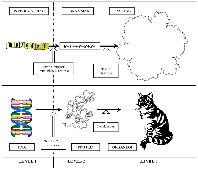
This procedure is similar in many respects to biological evolution. There are three different levels. Figure 1 shows a graphical scheme of the process in the particular case studied in this paper: the automatic generation of fractal curves with a given dimension.

• The genotype (nucleic acids), is represented in GE by vectors of integers.

• The intermediate level (proteins), is represented in GE by words in a given alphabet, which in our case describe an L system (see below). The translation from the genotype to the intermediate level is performed by means of a fixed grammar (the equivalent of the fixed genetic code).

• The phenotypic (organisms), in our case represented by the fractal curves obtained from the intermediate-level words by means of a graphical interpretation.

1.2 Fractals and fractal dimension

The concept of dimension is very old and seems easy and evident: sometimes it can be clearly and elegantly defined as the number of directions in which movement is allowed: with this interpretation, dimensions are consecutive integers: 0 (a point), 1 (a line), 2 (a surface), 3 (a volume), with no doubtful cases. This is called a topological dimension. However, as ? describe in his seminal article, some doubtful cases exist: depending on the size of the observer, a ball of thread can be considered as a point (dimension 0, for a large observer), a sphere (dimension 3, for an observer comparable to the ball), a twisted line (dimension 1, for a smaller observer), a twisted cylinder (dimension 2, for an even smaller observer), and so forth.

There is a class of apparently one-dimensional curves for which the concept of dimension is tricky: in 1890, Giuseppe Peano defined a curve which goes through every point in a square, and therefore can be considered as two-dimensional. In 1904, Helge von Koch devised another, whose shape reminds a snowflake and whose longitude is infinite, although the surface it encloses is limited. Von Koch’s snowflake does not fill a surface, therefore its dimension should be greater than 1 but less than 2. In 1919, Hausdorff proposed a new definition of dimension, applicable to such doubtful cases: curves such as those just described may have a fractional dimension, between 1 and 2. Peano’s curve has a Hausdorff dimension of 2; Von Koch’s snowflake has a Hausdorff dimension of 1.2618595071429… Other alternative definitions of dimension were proposed during the twentieth century, such as the Hausdorff-Besicovitch dimension, the Minkowsky dimension, or the boxcounting dimension (see ?, ?). They differ only in details and are known as fractal dimensions.

The name fractal was introduced in 1975 by Mandelbrot and applies to objects with some special properties, such as a fractal dimension different from their integer topological dimension, self-similarity (containing copies of themselves), and/or non-differentiability at every point.

Fractal curves have been generated or represented by different means, such as fractional Brownian movements, recursive mathematical families of equations (such as those that generate the Mandelbrot set), and recursive transformations (generators) applied to an initial shape (the initiator). They have found applications in antenna design, the generation of natural-looking landscapes for artistic purposes, and many other fields. The generation of fractals with a given dimension can be useful for some of these applications.

This paper discusses only the initiator-generator family of fractals.

1.3 L systems

L systems, devised by ?, also called parallel-derivation grammars, differ from Chomsky grammars because derivation is not performed sequentially (a single rule is applied at every step) but in parallel (every symbol is replaced by a string at every step). L systems are appropriate to represent fractal curves obtained by means of recursive transformations (?). The initiator maps to the axiom of the L system; the generator becomes the set of production rules; recursive applications of the generator to the initiator correspond to subsequent derivations of the axiom. The fractal curve is the limit of the word derived from the axiom when the number of derivations tends to infinity.

Something else is needed: a graphic interpretation which makes it possible to convert the words generated by the L system into visible graphic objects. Two different families of graphic interpretations of L systems have been used: turtle graphics and vector graphics. In a previous paper, we have proved an equivalence theorem between two families of L systems, one associated with a turtle graphics interpretation, the other with vector graphics (?). Our theorem makes it possible to focus only on turtle graphics without a significant loss of generality.

The turtle graphics interpretation was first proposed by ? as the trail left by an invisible turtle, whose state at every instant is defined by its position and the direction in which it is looking. The state of the turtle changes as it moves a step forward or as it rotates by a given angle in the same position. Turtle graphics interpretations may exhibit different levels of complexity. We use here the following version:

• The angle step of the turtle is $\alpha=(2k\pi/n)$, where $k$ and $n$ are two integers.

• The alphabet of the L system is expressed as the union of the four disjoint subsets: $N$ (non-graphic symbols), $D$ (visible graphic symbols, which move the turtle one step forward, in the direction of its current angle, leaving a visible trail), $M$ (invisible graphic symbols, which move the turtle one step forward, in the direction of its current angle, leaving no visible trail) and extra symbols such as $\{+,-\}$, which increase/decrease the turtle angle by $\alpha$, or a parenthesis pair, which are used in conjunction with a stack to add branches to the images. These symbols usually are associated with L system trivial rules such as $+::=+$. In the following, the trivial rules will be omitted but assumed to be present.

A string is said to be angle-invariant with a turtle graphics interpretation if the directions of the turtle at the beginning and the end of the string are the same. In this paper we only consider angle-invariant D0L systems (where D0L describes a deterministic context-free L system), i.e. the set of D0L systems such that the right-hand side of all of their rules is an angle-invariant string.

Summarizing: a fractal curve can be represented by means of two components: an L system and a turtle graphics interpretation, with a given angle step. The length of the moving step (the scale) is reduced at every derivation in the appropriate way, so that the curve always occupies the same space.

2 An algorithm to determine the dimension of a fractal curve from its equivalent L system

Several classic techniques make it possible to estimate the dimension of a fractal curve. All attempt to measure the ratio between how much the curve grows in length, and how much it advances. The ruler dimension estimation computes the dimension of a fractal curve as a function of two measurements taken while walking the curve in a number of discrete steps. The first measurement is the pitch length ($p_{l}$), the length of the step used, which is constant during the walk. The second is the number of steps needed to reach the end of the walk by walking around the fractal curve, $N\left(p_{l}\right)$. The fractal dimension, $D_{p_{l}}$, is defined as

$$D_{p_{l}}=\lim_{p_{l}\rightarrow 0^{+}}\frac{-\log N(p_{l})}{\log p_{l}}$$ (1)

In a previous work (?) we presented an algorithm that reaches the same result by computing directly from the L system that represents the fractal curve, without performing any graphical representation. The L system is assumed to be an angle-invariant D0L system with a single draw symbol. The production set consists of a single rule, apart from trivial rules for symbols $+$, $-$, $($, and $)$. Informally, the algorithm takes advantage of the fact that the right side of the only applicable rule provides a symbolic description of the fractal generator, which can be completely described by a single string. The algorithm computes two numbers: the length $N$ of the visible walk followed by the fractal generator (equal in principle to the number of draw symbols in the generator string), and the distance $d$ in a straight line from the start to the endpoint of the walk, measured in turtle step units (this number can also be deduced from the string). The fractal dimension is:

$$D=\frac{\log N}{\log D}$$ (2)

The scale is reduced at every derivation in such a way that the distance between the origin and the end of the graphical representation of the strings is always the same. For instance, the D0L scheme associated with the rule

$F::=F+F--F+F$

with axiom $F--F--F$ and a turtle graphic interpretation, where ${F}$ is a visible graphic symbol and the step angle is 60, represents the fractal whose fifth derivation appears in figure 2.

Figure 2: Von Koch snowflake curve.

The string $F+F--F+F$ describes the fractal generator. The number of steps along the walk ($N$) is the number of draw symbols in the string, 4 in this case. The distance $d$ between the extreme points of the generator, computable from the string by applying the turtle interpretation, is 3. Therefore, the dimension is

$$D=\frac{\log 4}{\log 3}=1.2618595074129\ldots$$ (3)

This is the same dimension obtained with other methods, as specified in (?, p. 42).

This algorithm can be easily extended to fractals whose L systems contain more than one draw symbol and more than one rule, if all the rules preserve the ratio between $N$ and $d$ in the previous expression. Most of the initiator-iterator fractals found in the literature can be represented by angle-invariant D0L systems whose draw symbols-contribute to the dimension in this way. The algorithm was also refined to successfully include fractal curves which overlap, either in the generator itself, or after subsequent derivations. In those cases, the definition of the fractal dimension is replaced by

$$D=\lim\frac{\log N}{\log d}$$ (4)

where the limit is taken when the number of derivations goes to infinity. Our algorithm computes this case by computing the dimension of a certain number of derivations until the quotient converges.

3 Grammatical evolution to design fractal curves with a given dimension

Designing fractal curves with a given dimension is relatively easy for certain values of the desired dimension (for instance, 1.261858… or $\log 4/\log 3$), but very difficult for others (the reader can try to hand design a fractal curve with a dimension of 1.255). To do it, one has to find two integer numbers, $a$ and $b$, such that 1.255 = $\log a/\log b$. Then one has to design a geometrical iterator such that it would take $a$ steps to advance a distance equal to $b$.

This problem can be solved automatically by means of grammatical evolution. Our genetic algorithm acts on genotypes consisting of vectors of integers and makes use of a fixed grammar to translate the genotypes into an intermediate level, which can be interpreted as a single rule for an L system which, together with a turtle graphic interpretation, generates the final phenotype: a fractal curve with a dimension as approximate as desired to the desired value. The algorithm can be described as follows:

1. Generate a random population of 64 vectors of eight integers in the $[0,10]$ or the $[0,255]$ interval (the latter case introduces genetic code degeneracy). All the genotypes in the initial population have the same length. Subsequent populations may contain individuals with genotypes of different lengths.

2. Translate every individual genotype into a word in the alphabet $F,+,-$ as indicated below.

3. Using the algorithm described in section 3, compute the dimension of the fractal curve represented by the D0L system which uses the preceding word as a generator.

4. Compute the fitness of every genotype as $(\text{target}-\text{dimension})^{-1}$.

5. Order the 64 genotypes from higher to lower fitness.

6. If the highest-fitness genotype has a fitness higher than the target fitness, stop and return its phenotype.

7. From the ordered list of 64 genotypes created in step 5, remove the 16 genotypes with least fitness (leaving 48) and take the 16 genotypes with most fitness. Pair these 16 genotypes randomly to make eight pairs. Each pair generates another pair, a copy of their parents, modified according to four genetic operations (see below). The new 16 genotypes are added to the remaining population of 48 to make again 64, and their fitness is computed as in steps 2 to 4.

8. Go to step 5.

The algorithm has three input parameters: the target dimension (used in step 4), the target minimum fitness (used in step 6) and the angle step for the turtle graphics interpretation (used in step 3).

In step 2, the following grammar is used to translate the genotype of one individual into its equivalent intermediate form (the generator for an L system representing a fractal curve):

$0:F::=F$

$1:F::=FF$

$2:F::=F+$

$3:F::=F-$

$4:F::=+F$

$5:F::=-F$

$6:F::=F+F$

$7:F::=F-F$

$8:F::=+$

$9:F::=-$

$10:F::=\lambda$

The translation is performed according to the following developmental algorithm:

1. The axiom (the start word) of the grammar is assumed to be $F$.

2. As many elements from the remainder of the genotype are taken (and removed) from the left of the genotype as the number of times the letter $F$ appears in the current word. If there remain too few elements in the genotype, the required number is completed circularly.

3. Each $F$ in the current word is replaced by the right-hand side of the rule with the same number as the integers obtained by the preceding step. With genetic code degeneracy, the remainder of each integer modulo 11 is used instead. In any derivation, the trivial rules $+::=+$ and $-::=-$ are also applied.

4. If the genotype is empty, the algorithm stops and returns the last derived word.

5. If the derived word does not contain a letter $F$, the whole word is replaced by the axiom.

6. Go to step 2.

The four genetic operations mentioned in step 7 of the genetic algorithm are the following:

• Recombination (applied to all the generated genotypes). Given a pair of genotypes, $(x_{1},x_{2},...,x_{n})$ and $(y_{1},y_{2},...,y_{m})$, a random integer is generated in the interval $[0,\min(n,m)]$. Let it be $i$. The resulting recombined genotypes are $(x_{1},x_{2},...,x_{i-1},y_{i},y_{i+1},...,y_{m})$ and
  $(y_{1},y_{2},...,y_{i-1},x_{i},x_{i+1},...,x_{n})$.

• Mutation, applied to $n_{1}$ per cent of the generated genotypes if both parents are equal, to $n_{2}$ per cent if they are different. It consists of replacing a random element of the genotype vector by a random integer in the same interval.

• Fusion, applied to $n_{3}$ per cent of the generated genotypes. The genotype is replaced by a catenation of itself with a piece randomly broken from either itself or its brother’s genotype. (In some tests, the whole genotype was used, rather than a piece of it.)

• Elision, applied to 5 per cent of the generated genotypes. One integer in a random position of the vector is eliminated. The last two operations make it possible to generate longer or shorter genotypes from the original eight element vectors.

4 Heavy tail distributions

Heavy tail distributions are probabilistic distributions which exhibit an asymptotic hyperbolic decrease, usually represented as

$$\Pr\{|X|>x\}\sim Cx^{-\alpha},$$ (5)

where $\alpha$ is a positive constant. Distributions with this property have been used to model ramdom variables whose extreme values are observed with a relatively high probability.

Work on these probability distributions can be traced to Pareto’s (?) work on the earning distribution or to Levy’s (?) work on the properties of stable distributions. A fundamental advance in the use of heavy tail distributions for was provided by Mandelbrot’s work (?, ?) on the application of fractal behavior and self-similarity to the modeling of real-world phenomena, which he used to introduce stable distributions to model price changes in the stock exchange. Heavy tail distributions have also been used in areas such as statistical physics, wheather prediction, earthquake prediction, econometrics and risk theory (?, ?). In more recent times, these distributions have been used to model waiting times in the World Wide Web (?) or the computational cost of random algorithms (?, ?, ?, ?).

For many purposes, the only relevant parameter of a heavy tail distribution is its characteristic exponent $\alpha$, which determines the ratio of decrease of the tail and the probability of occurrence of extreme events. In this work we only consider heavy tail distributions where $\alpha$ belongs to the $(0,2)$ interval, with positive support ($\Pr\{0\leq X<\infty\}=1$).

The existence or inexistence of the different moments of a distribution is fully determined by the behavior of its tail: $\alpha$ can also be regarded as the exponent of the maximum finite moment of the distribution, in the sense that moments of $X$ of order less than $\alpha$ are finite, while moments of order equal or greater are infinite. For instance, when $\alpha=1.5$, the distribution has a finite average and an infinite variance, while for $\alpha=0.6$ both average and variance are infinite.

4.1 Estimation of the characteristic exponent

Many procedures have been used to estimate $\alpha$ (?, ?, ?). Two of them have received the most extensive usage. The first uses a maximum likelihood estimator, the second applies a simple regression method.

An important issue while estimating $\alpha$ is how to tackle censored observations when extreme data are not available. Consider, for instance, physical phenomena such as wind velocity or earthquake magnitude, where heavy tail distributions have been considered appropriate. In these cases, extreme measures are non-observable, since very strong hurricanes or highly destructive earthquakes will damage the measuring instruments. In the process of financial data, such as stock exchange rates, heavy tail models have also been used (?). In moments of high volatility, when extreme data usually appear, many stock exchange markets introduce rules to limit transactions or even close the market, to prevent them from taking place. Consider finally the case of random algorithms: the computational costs of some problems are so high, that the algorithms have no alternative but to interrupt the execution and start again with a different random seed. In those cases, computational costs are not observable beyond a certain threshold (?). Thus the censorship of extreme values needs to be considered by available estimators.

Let $X_{n1}\leq X_{n2}\leq\ldots X_{nn}$ be the ordered statistics, i.e. the ordered values in the sample $X_{1},X_{2},\ldots,X_{n}$. Let $r<n$ be the truncation value which separates normal from extreme observations.

The adapted Hill-Hall estimator for censored observations is:

$$\hat{\alpha}_{r,u}=(\frac{1}{r}\sum_{j=1}^{r-1}\ln X_{n,n-r+j}+\frac{u+1}{r}\ln X_{n,n}-\frac{u+r}{r}\ln X_{n,n-r})^{-1}.$$ (6)

In this notation, $n$ is the number of observed data, $r+1$ is the number of larger observations selected and $u$ is the number of non-observed extreme values. If all the data are observable, $u=0$ and equation (6) becomes the classic Hill-Hall estimator.

In heavy tail distributions, the ratio of decay of the estimated density is hyperbolic (slower than a exponential decay). Thus the one-complement of the accumulated distribution function, $\overline{F}(\cdotp)$, also shows a hyperbolic decay.

$$\overline{F}(x)=1-F(x)=\Pr\{X>x\}\sim Cx^{-\alpha}.$$ (7)

Therefore, for a heavy-tail variable, a log-log graph of the frequency of observed values larger than $x$ should show an approximately linear decay in the tail. Moreover, the slope of the linear decaying graph is in itself an estimation of $\alpha$. This can be contrasted with a exponentially decaying tail, where a log-log graph shows a faster-than-linear tail decay.

This simple property, besides giving visual evidence of the presence of a heavy tail, also gives place to a natural regression estimator based on equation 7, the least-squares estimator (?), which can be expressed in terms of a selected number of extreme observations. Assume that we have a sample of $k=n+u$ independent identically distributed random variables. Assume also that we only observe the $n$ smallest values of random variable $X$ and therefore have the ordered statistics $X_{n1}\leq X_{n2}\leq\ldots\leq X_{nn}$. Assume that, for $X_{n,n-r}\leq X\leq X_{nn}$, the tail distribution has a hyperbolic decay. The least-square regression estimator for the $\alpha$ exponent is

$$\hat{\alpha}=-\frac{\sum l_{i}\log X_{ni}-\sum l_{i}\sum\log X_{ni}/(r+1)}{\sum(\log X_{ni})^{2}-\sum(\log X_{ni})^{2}/(r+1)},$$ (8)

where $l_{i}=\log\frac{n+u-i}{n+u}$ and the sums go from $i=n-r$ to $i=n$. If all the values in the sample $k=n+u$ can be observed, then $u=0$ and $k=n$.

4.2 Leptokurtic distributions vs. heavy tail distributions

The name heavy tail, applied to a class of distributions, expresses their main property: the large proportion of total probability mass concentrated in the tail, which reflects its (hyperbolic) slow decay and is the reason why all the moments of a heavy tail distribution are infinite, starting at a given order.

The concept of kurtosis is also related to the tail heaviness. The kurtosis of a distribution is the amount $\mu_{4}/\mu_{2}^{2}$, where $\mu_{2}$ and $\mu_{4}$ are the second and fourth centralized moments ($\mu_{2}$ is the variance). The kurtosis is independent of the localization and scale parameters of a distribution. Kurtosis is high, in general, for a distribution with a high central peak and long tails.

Figure 3: Low kurtosis vs. high kurtosis. The probability density function on the right has a higher kurtosis than the left: its center part has a higher peak and its tails are heavier.

The kurtosis of the standard normal distribution is 3. A distribution with a kurtosis higher than 3 is called leptokurtic as opposite to platokurtic (see fig. 3) . In a similar way to heavy tail distributions, a leptokurtic distribution has long tails with a considerable concentration of probability. However, the tail of a leptokurtic distribution decays faster than that of a heavy tail distribution: all the moments in a leptokurtic distribution can be finite, in a strong contrast with a heavy tail distribution where, at most, the first two moments are finite.

5 Heavy tails in Grammatical Evolution

Randomized algorithms with a high execution time variability are suspetc of hiding a heavy tail distribution. In the present section we provide empirical evidence that our GE algorithm for the automatic generation of fractal curves may exhibit a heavy tail behavior which can be exploited to improve the performance.

dimension	angle (degrees)	# experiments	# generations range
1.1	45	10	[37, 9068]
1.1	60	4	[119, 72122]
1.2	45	8	[188, 11173]
1.2	60	10	[21, 750]
1.3	45	9	[50, 18627]
1.3	60	4	[14643, 66274]
1.25	60	2	[1198, 3713]
1.255	60	15	[1, 2422]
1.2618595…	60	4	[1, 2]
1.4	45	10	[79, 781]
1.4	60	10	[33, 1912]
1.5	45	11	[52, 11138]
1.5	60	8	[12, 700]
1.6	45	5	[275, 3944]
1.6	60	1	[116, 913]
1.7	45	2	[585, 1456]
1.7	60	8	[18, 1221]
1.8	45	2	[855, 2378]
1.8	60	13	[69, 3659]

Table 1: Number of generations needed to generate a fractal curve with a given dimension in a set of experiments.

? provides data about different executions of the same algorithm to generate fractal curves with the same dimensions, using different random seeds. The numbers of generations needed to reach the target differ in up to two orders of magnitude (see table 1).

Figure 4: Empirical distribution function of the number of generations needed to reach a solution for several fractal dimensions: 1.3, 1.5, 1.8 and 2.

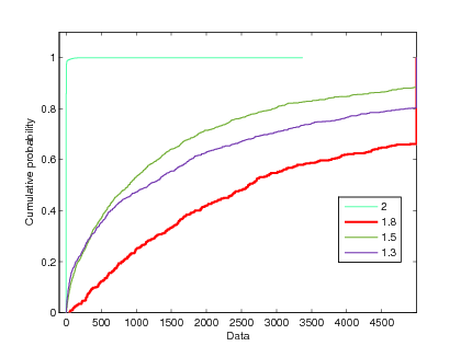
Figure 4 shows the empirical distribution of the number of generations needed to find a solution, i.e.

$$F(x)=\Pr\{\text{number of generations to reach a solution}\leq x\}$$ (9)

for four different fractal dimensions: 1.3, 1.5, 1.8 and 2. The empirical distribution functions have been obtained by running 1,000 executions with 1,000 different independent random seeds. At the end of each execution, the number of generations needed to reach a solution is recorded. We took a censorship value equal to $\tau=5,000$ generations, meaning that, if an execution needs over 5,000 generations, it is stopped and marked as non-observable.

dimension	1.3	1.5	1.8	2
observable	80.5%	88.3%	66.2 %	100%
non-observable	19.5%	12.7%	38.2 %	0%

Table 2: Percentages of observable and non-observable executions for a censorship value $\tau=5,000$ generations.

Table 2 shows the percentages of non-observable executions in our experiments. This percentage is quite high, specially for dimensions 1.8 and 1.3. The empirical distribution functions may be used to test whether the distribution has a heavy tail.

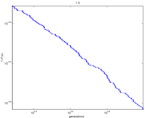
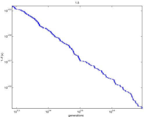
In the previous section (definition 5) we saw that a random variable has a heavy tail behavior if it shows an asymptotic hyperbolic decay, although that behavior can also be shown in its whole support. In the figures displayed in this section, only the extreme values are shown, therefore we had to choose a parameter $r$ to truncate the non-extreme observations. Usually $r$ takes values in the $[1\%,25\%]$ interval; we will use the set {1%, 2.5%, 5%, 10%, 15%, 20%}, as recommended by ?.

Figure 5: Log-log graph of the tail of ($r$=20%) distributions for dimensions 1.3, 1.5, 1.8 and 2.

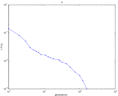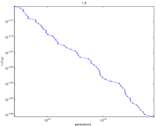
Figure 5 shows the log-log graphs of the distribution tails for fractal dimensions 1.3, 1.5, 1.8 and 2. Notice the linear decay of function $\log\overline{F}(x)$, in contrast with exponential decay distributions, where the decay of $\log\overline{F}(x)$ is faster than linear.

Figure 6: Box-and-whisker type graphs for dimensions 1.3, 1.5, 1.8 and 2.

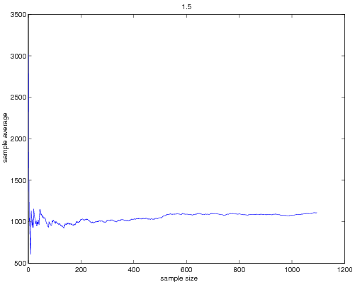
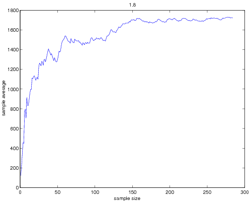
The averages for dimensions 1.3, 1.5 and 1.8 are $E(X_{1.3})=1,173$, $E(X_{1.5})=1,108$ and $E(X_{1.8})=1,721$. It can be seen that, with a number of generations almost 5 times above their averages, respectively over 10%, 20% and 30% executions have not finished.

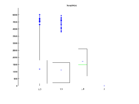
Figure 6 displays four box-and-whisker graphs, which give rise to three remarkable conclusions:

• The median (the dashed line within the box in fig. 6) is much smaller than the average (the cross ‘+’ within the box) for dimensions 1.3, 1.5 and 1.8. This suggests that the average of these distributions is biased by the size of the sample, which means that they may have an infinite asymptotic average typical of heavy tail distributions.

• The sample distribution is strongly biased towards high execution times, indicating a right-hand-side heavy tail. This can be seen in the fact that the lower interquartilic distance (the difference between the first quartile - the lower segment of the box - and the the median - the green line) is shorter than the upper interquartilic distance (the difference between the median and the third quartile - the upper segment of the box). Besides this, the distance between the minimum and the first quartile is much less than the distance between the maximum (the highest point of the graph) and the third quartile.

5.1 Estimating the characteristic exponent

The preceding section provides visual evidence for a heavy tail behavior in dimensions 1.3, 1.5, 1.8. Evidence for this behavior is weaker in dimension 2, but also present in, for instance, the linear decay observed in figure 5. In this section we estimate the characteristic exponent for these distributions, using the estimators presented in section 4.

First we compute the Hill-Hall estimator adapted for censored observations, (equation 6).

dimension	$r$
	1%	2.5%	5%	10%	15%	20%
1.3	0.7827	0.6796	0.8312	0.7953	0.7634	0.7084
1.5	1.1765	1.2400	1.0952	1.0595	0.9952	0.9418
1.8	0.3649	0.4855	0.6746	0.5759	0.5657	0.5705
2	0.7656	0.6043	1.0403	1.0463	0.7732	1.0309

Table 3: Estimations of $\alpha$ for dimensions 1.3, 1.5, 1.8 and 2 using the adapted Hill-Hall estimator.

Table 3 confirms that these distributions are heavy tailed, since all the values in the table are less than 2, the limit for heavy tail distributions.

For dimension 1.3, all the estimations (for all values of $r$) are less than 1, which means that this distribution does not have neither a finite average nor a finite variance. The same happens for dimension 1.8 even in a stronger way, as the values of $\alpha$ are even smaller (all are below 0.7).

Dimensions 1.5 and 2 provide examples of heavy tail distributions with a characteristic exponent $\alpha$ between 1 and 2. These distributions have a finite average, but an infinite variance, indicating that their right heavy tail is lighter than in the other two distributions.

Figure 7: Evolution of the sample average as a function of the sample size for dimensions 1.3, 1.5, 1.8 and 2.

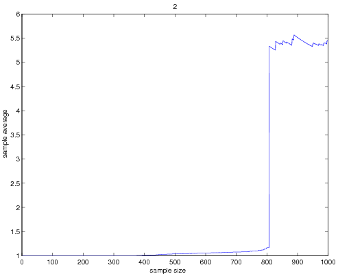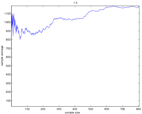
Figure 7 displays the erratic behavior of the sample average as a function of the sample size.

dimension	$r$
	1%	2.5%	5%	10%	15%	20%
1.3	0.6952	0.7528	0.7715	0.7904	0.7692	0.7345
1.5	1.1318	1.3790	1.0886	0.9664	0.9786	0.9721
1.8	0.3310	0.5220	0.7285	0.6424	0.5762	0.5762
2	$\approx$0	$\approx$0	0.2554	0.4821	0.6008	0.6667

Table 4: Estimations of $\alpha$ for fractal dimensions 1.3, 1.5, 1.8 and 2, using the regression estimator.

To verify the reliability of our characteristic exponent estimation, table 4 shows the estimations obtained using the regression estimator described in a previous section (equation 8), which is considered slightly less robust than the maximum likelihood estimator (adapted Hill-Hall). The results of this estimator can be seen to be consistent with those of the adapted Hill-Hall estimator.

5.2 Tail truncation

As mentioned before, in practice one has to select the GE maximum number of generations for specially difficult problems. In other words, an appropriate censorship value $\tau$ must be chosen, so that the algorithm does not become stagnated in the extreme values of the distribution tail. As a consequence, the tail is truncated. The selection of the value of $\tau$ depends on the problem and the algorithm. Ideally, only a small portion of tail should be truncated, but this may be prohibitive from the computational point of view.

If the truncation is set at a small number of generations, it will be harder to distinguish between heavy tail and leptokurtic distributions. From a practical point of view, this is not a problem, if there are strong indications that the tail exhibits at least one of the two behaviors. A heavy tail behavior is not a necessary condition to accelerate randomized search methods. In fact, it has been proved that the efficiency of the search in leptokurtic distributions can be improved by randomized backtracking (?). However, with a heavy tail distribution, the occurrence of long executions will be more frequent than with a leptokurtic distribution, making it possible to obtain a higher potential acceleration.

dimension	1.3	1.5	1.8	2
$\mu_{2}$	1.6171e+06	1.3532e+06	1.5496e+06	69.9039
$\mu_{4}$	9.0640e+12	7.6389e+12	6.0015e+12	9.6330e+05
$\text{kurt}(x)$	3.4575	4.1642	2.4817	197.1335

Table 5: Kurtosis computation for dimensions 1.3, 1.5, 1.8 and 2.

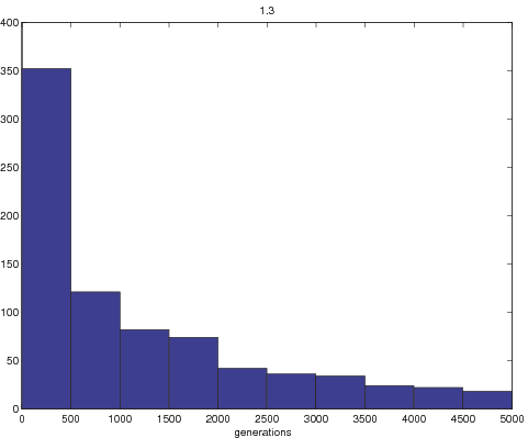
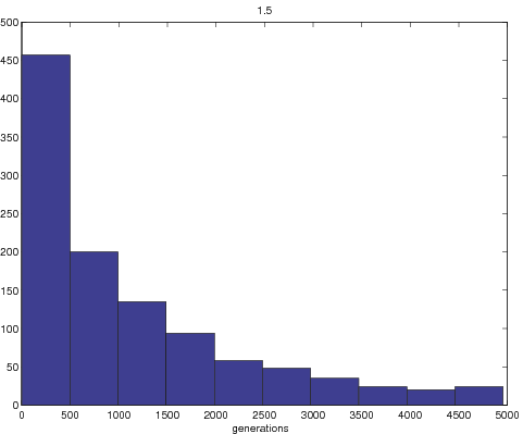
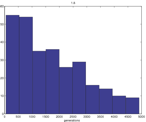
Table 5 shows the kurtosis for the 4 fractal dimensions considered. Remember that, if this value is greater than 3 (the kurtosis for a normal distribution) the distribution is leptokurtic (with abrupt peaks and heavy tails), otherwise it is platokurtic (with smooth peaks and light tails). In our case, fractal dimensions 1.3, 1.5 and 2 are seen to be leptokurtic, while dimension 1.8 is platokurtic. Figure 8 shows the histograms built for the execution samples for dimensions 1.3, 1.5, 1.8 and 2.

Figure 8: Histograms with the execution samples obtained for fractal dimensions 1.3, 1.5, 1.8 and 2.

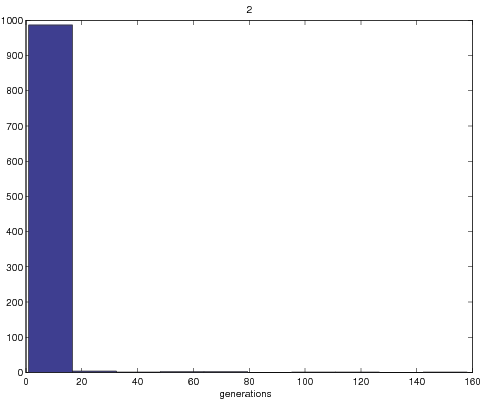This section ends with the conclusion that there exists an application of GE, automatic fractal generation, whose distributions exhibit a heavy tail behavior, besides being leptokurtic in many cases. In the next section we show that it is possible to take advantage of this probabilistic characterization to increase the performance of GE and yield a fast fractal generation algorithm.

6 Restart strategies

We have shown that our algorithm may give rise to computational efforts with a leptokurtic or heavy tail distribution. This may be due to the fact that the algorithm makes bad choices more frequently than expected, leading the search to a dead-end in the search space, where no solution of the required fitness exists.

The algorithm seems to be more efficient at the beginning of the search, which suggests that a sequence of short executions, compared to a single long execution, may give rise to a better use of the computational resources. In this section we show that the algorithm may be accelerated by the use of several restart strategies.

6.1 Restarts with a fixed threshold

Figure 9: Function $F(x)$ for several values of the restart threshold $\theta\in\{10,20,50,\infty\}$ applied to fractal dimension 1.3.

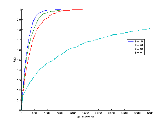
Figure 9 displays the result of a restart strategy with a fixed threshold applied to the generation of a fractal curve with dimension 1.3. This is the simplest strategy: once the algorithm has been working for a predefined number of generations $\theta$, without reaching the desired goal, a new execution is started with a different random seed. As the figure shows, the failure rate after 500 generations is 70% ($F(500)=0.3$), while this percentage falls to 10% using restarts with a threshold $\theta=10$ generations.

Such an improvement is typical of heavy tail distributions. The fact that the experimental curve has been so dramatically moved towards the beginning of the support is a clear indication that the heavy tail character of the original distribution has disappeared in the modified algorithm.

Figure 10: Function $F(x)$ for several values of the restart threshold $\theta\in\{10,20,50,\infty\}$ applied to fractal dimension 1.5.

Figure 11: Function $F(x)$ for several values of the restart threshold $\theta\in\{500,1000,2000,\infty\}$ applied to fractal dimension 1.8.

Figure 12: Function $F(x)$ for several values of the restart threshold $\theta\in\{1,2,5,\infty\}$ applied to fractal dimension 2.

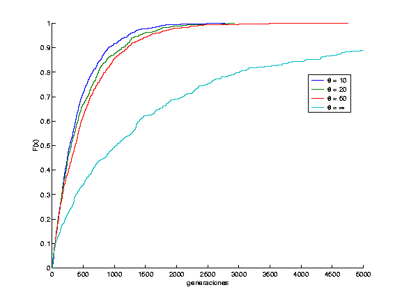
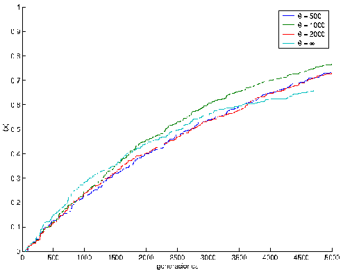
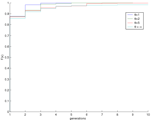
Figures 10, 11 and 12 clearly show that the restarts make the tail of the distributions lighter, thus providing a mechanism to handle heavy tail and leptokurtic distributions.

$\theta$	% solved	average cost
2	100%	382.6740
4	100%	277.5730
8	100%	207.8240
16	100%	271.3980
32	100%	345.2680
64	100%	407.2460
128	100%	621.1770
256	99.8%	830.4220
512	98.5%	985
1024	96.4%	1,367
2048	93.7%	1,909

Table 6: Percentage solved and average cost for several threshold values in the fractal dimension 1.3 experiment.

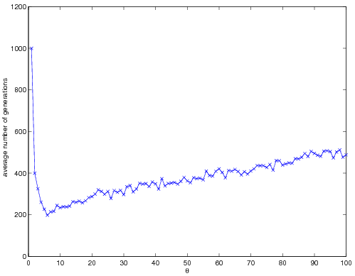
Different fixed thresholds give rise to different average times needed to reach a solution. Table 6 and figure 13 show that the threshold value $\theta=6$ minimizes the expected cost for fractal dimension 1.3, making it the optimal threshold $\theta^{*}$. For threshold values larger than the optimal, the heavy tail behavior at the right of the median dominates the average cost, while below the optimal value the success percentage is too small and too many restarts are required. Anywhere, many non-optimal choices provide a considerable acceleration of the algorithm.

It has been proven that the use of a fixed restart threshold $\theta$ with a heavy tail distribution eliminates this behavior in such a way that all the moments of the new distribution become finite (?).

Figure 13: The effect of restarts with fixed $\theta$ on the solution costs for fractal dimension 1.3.

6.2 Restart sequences

The idea of a fixed threshold comes from theoretical results by ?, which describe optimal restart policies. It can be proven that if the time distribution of the execution is completely known and therefore $\theta^{*}$ can be calculated a priori, restarting every $\theta^{*}$ generations yields the minimum average execution time.

? also provide a strategy (a universal strategy applicable to every distribution) to minimize the expected cost of random procedures in the case where no a priori knowledge is available. It consists of sequences of executions whose values are powers of two. After two executions with a given threshold, the threshold is changed to its double value. Let $t_{i}$ be the number of generations of the i-th execution; the universal strategy is defined as:

$$t_{i}=\begin{cases}2^{k-1}&\text{if}\ i=2^{k}-1\\ t_{i-2^{k-1}+1},&\text{if}\ 2^{k-1}\leq i<2^{k}-1,\end{cases}$$

yielding strategies of the form

$$(1,1,2,1,1,2,4,1,1,2,1,1,2,4,8,1,\ldots).$$

? presents two theorems which together prove the asymptotic optimality of this procedure for an unknown distribution.

Table 7 summarizes the results of the application of both strategies. The average time using restarts with the universal strategy is approximately twice the time needed using fixed restarts with the optimal threshold. Both yield a considerable acceleration against the algorithm without restarts.

dimension	no restart	optimal fixed threshold		universal
1.3	1,173	164.	9655 $(\theta^{*}=6)$	294.867
1.5	1,108	374.	2069 $(\theta^{*}=10)$	622.181
1.8	1,443	248.	5263 $(\theta^{*}=17)$	625.334
2	5.4360	1.	1655 $(\theta^{*}=1)$	1.1701

Table 7: A comparison between average execution times for each dimension without restarts, with an optimal fixed threshold strategy and with the universal strategy.

In several problems whose execution times had heavy tail distributions, the universal strategy was found to grow ‘too slowly.’ This happens because, in those problems, the restart sequence takes too many iterations to reach a value near $\theta^{*}$ (?, ?). A correction was proposed by ?, with a new restart strategy which was applied successfully to constraint satisfaction problems. In this simple strategy, each new restart is a constant factor $\gamma$ greater than the preceding value:

$$(1,\gamma,\gamma^{2},\gamma^{3},\ldots),\quad\gamma>1.$$ (10)

This strategy has a high probability of success when the restart value $t_{i}=\gamma^{i-1}$ is near the optimal restart threshold value. Increasing the restart threshold geometrically makes sure that the optimal value will be reached in a few generations. The solution is expected to be found within a few restarts after the value of $t_{i}$ has surpassed the optimal. This strategy has the advantage of being less sensitive to the actual distribution it is applied to.

Figure 8 displays the average execution times using Walsh strategy for several values of $\gamma$. It can be seen that $\gamma=1.2$ provides the fastest acceleration; with this parameter, fractal dimension 2 reaches the performance of fixed restarts with optimal threshold. The average times for fractal dimensions 1.3 and 1.5 are approximately double of those obtained with the universal strategy, although much less than those without any restart strategy. A special case is fractal dimension 1.8, where Walsh strategy worsens the performance.

dimension	Walsh
	$\gamma=1.2$	$\gamma=1.4$	$\gamma=1.6$	$\gamma=1.8$	$\gamma=2$
1.3	441.5138	639.0714	846.0743	773.4603	898.4630
1.5	654.5434	773.9020	845.0908	905.0780	938.3790
1.8	3,115	2,695	2,527	2,437	2,372
2	1.167	1.1827	1.1729	1.1979	1.1783

Table 8: Average execution times using the Walsh strategy for several values of $\gamma$.

7 Conclusions and future work

Heavy tail probability distributions have been used to model several real world phenomena, such as weather patterns or delays in large communication networks. In this paper we have shown that these distributions may be also suitable to model the execution time of an algorithm which uses Grammatical Evolution for automatic fractal generation. Heavy tail distributions help to explain the erratic behavior of the mean and variance of this execution time and the large tails exhibited by the distribution.

We have proved that restart strategies mitigate the inconveniences associated with heavy tail distributions and yield a considerable acceleration on the previous algorithm. These strategies exploit the non-negligible probability of finding a solution in short executions, thus reducing the variance of the execution time and the possibility that the algorithm fails, which improves the overall performance.

We have given evidence that several restart strategies are of practical value, even in scenarios with no a priori knowledge about the probability distribution of the execution time.

So far, we have considered situations of complete or inexistent knowledge. In real situations, the execution time or the resources are bounded, so that some partial knowledge about the execution time is available. In this scenario, we suspect that our algorithm would take advantage of dynamic restart strategies based on predictive models, which have been used successfully to tackle decision and combinatorial problems (?, ?, ?). Further research along this line would be focused on pinpointing the real time knowledge about the behavior of the algorithm which would make it possible to build predictive models for its execution time, thus providing a further acceleration.

Finding the conditions for the execution time of a particular Grammatical Evolution experiment to exhibit a heavy tail distribution would also make an interesting research line: is the fractal generation optimization exhibiting a typical behavior or just an exception?