Cosmic velocity–gravity relation in redshift space

Abstract

We propose a simple way to estimate the parameter $\beta\simeq\Omega^{0.6}/b$ from three-dimensional galaxy surveys, where $\Omega$ is the non-relativistic matter density parameter of the Universe and $b$ is the bias between the galaxy distribution and the total matter distribution. Our method consists in measuring the relation between the cosmological velocity and gravity fields, and thus requires peculiar velocity measurements. The relation is measured directly in redshift space, so there is no need to reconstruct the density field in real space. In linear theory, the radial components of the gravity and velocity fields in redshift space are expected to be tightly correlated, with a slope given, in the distant observer approximation, by

$$\frac{g}{v}=\frac{\sqrt{1+6\beta/5+3\beta^{2}/7}}{\beta}.$$

We test extensively this relation using controlled numerical experiments based on a cosmological $N$-body simulation. To perform the measurements, we propose a new and rather simple adaptive interpolation scheme to estimate the velocity and the gravity field on a grid.

One of the most striking results is that nonlinear effects, including ‘fingers of God’, affect mainly the tails of the joint probability distribution function (PDF) of the velocity and gravity field: the $1$–$1.5\sigma$ region around the maximum of the PDF is dominated by the linear theory regime, both in real and redshift space. This is understood explicitly by using the spherical collapse model as a proxy of nonlinear dynamics.

Applications of the method to real galaxy catalogs are discussed, including a preliminary investigation on homogeneous (volume limited) “galaxy” samples extracted from the simulation with simple prescriptions based on halo and sub-structure identification, to quantify the effects of the bias between the galaxy distribution and the total matter distribution, as well as the effects of shot noise.

1 Introduction

Analyzes of large-scale structure of the Universe provide estimates of cosmological parameters that are complementary to those from the cosmic microwave background measurements. In particular, comparing the large-scale distribution of galaxies to their peculiar velocities enables one to constrain the quantity $\beta\equiv\Omega^{0.6}/b$. Here, $\Omega$ is the cosmological non-relativistic matter density parameter and $b$ is the linear bias of galaxies that are used to trace the underlying mass distribution. This is so because the peculiar velocity field, ${\bf v}$, is induced gravitationally and is therefore tightly coupled to the matter distribution. In the linear regime, this relationship takes the form (Peebles 1980)

$${\bf v}({\bf r})=\Omega^{0.6}\int\frac{{\rm d}^{3}{\bf r}^{\prime}}{4\pi}\delta({\bf r}^{\prime})\frac{{\bf r}^{\prime}-{\bf r}}{|{\bf r}^{\prime}-{\bf r}|^{3}}\,,$$ (1)

where $\delta$ denotes the mass density contrast and distances have been expressed in $\hbox{km}\cdot\hbox{s}^{-1}$. Under the assumption of linear bias $\delta=b^{-1}\delta^{(g)}$, where $\delta^{(g)}$ denotes the density contrast of galaxies, the amplitude of peculiar velocities depends linearly on $\beta$.

Density–velocity comparisons are done by extracting the density field from full-sky redshift surveys (such as the PSCz, Saunders et al. 2000; or the 2MRS, Erdo$\breve{\rm g}$du et al. 2006), and comparing it to the observed velocity field from peculiar velocity surveys (such as the Mark III catalog, Willick et al. 1997; ENEAR, da Costa et al. 2000; and more recently SFI++, Masters et al. 2005). The methods for doing this fall into two broad categories. One can use equation (1) to calculate the predicted velocity field from a redshift survey, and compare the result with the measured peculiar velocity field; this is referred to as a velocity–velocity comparison (e.g., Kaiser et al. 1991; Willick & Strauss 1998). Alternatively, one can use the differential form of this equation, and calculate the divergence of the observed velocity field to compare directly with the density field from a redshift survey; this is called a density–density comparison (e.g., Dekel et al. 1993; Sigad et al. 1998). The advantage of density–density comparisons is that they are purely local, but they are significantly sensitive to shot noise because the divergence of the observed velocity field is estimated from the sparse velocity sample. The integral form of velocity–velocity comparisons make them much less sensitive to such a noise, but their non-local nature make them affected by the tides due to the presence of fluctuations outside the survey volume (see, e.g., Kaiser & Stebbins 1991).

Still, the common problem with both types of these comparisons is that while equation (1) involves the density field in real space, the observed density field is given solely in redshift space. One approach to tackle with this problem is to reconstruct the real-space density field from the redshift-space one. The transformation from the real space coordinate, ${\bf r}$, to the redshift space coordinate, ${\bf s}$, is

$${\bf s}={\bf r}+v({\bf r})\,\hat{{\bf r}}\,,$$ (2)

where $v({\bf r})={\bf v}\cdot\hat{{\bf r}}$; ${\bf v}({\bf r})$ is the real-space velocity field, and velocities are measured relative to the rest frame of CMB. Therefore, one has to correct galaxy positions for their peculiar velocities. To do so, equation (1) is used and a self-consistent solution for the density field in real space is usually obtained iteratively (Yahil et al. 1991). In the first iteration, to predict peculiar velocities according to equation (1), the real-space density field appearing on the r.h.s. of this equation is approximated by the redshift space-density field, and so on, until convergence. However, from equation (1) it is obvious that the amplitude of peculiar velocities depends on $\beta$, the parameter to be subsequently estimated. Therefore, to perform a density–velocity comparison self-consistently, one has to reconstruct the real space density field for a range of different values of $\beta$. For example, Branchini et al. (1999) performed such reconstructions for 10 different values of $\beta$ in the range $0.1$–$1.0$. Note that instead of this traditional algorithm, more sophisticated methods now rely on Euler-Lagrange action minimization (e.g., Peebles 1989; Shaya, Peebles & Tully 1995; Nusser & Branchini 2000; Phelps 2002; Phelps et al. 2006) or resolution of optimal assignement problems (e.g., Croft & Gaztañaga 1997; Frisch et al. 2002; Mohayaee et a. 2003; Mohayaee & Tully 2005).

Another approach, proposed by Nusser & Davis (1994; hereafter ND), is to perform the comparison directly in redshift space. ND derived the density–velocity relation in redshift space in the linear regime. Because velocity–velocity comparisons seem in practice more robust than density–density ones, they aimed at transforming this relation to an integral form, i.e. at solving for the velocity as a functional of the redshift-space density. Due to the radial character of redshift-space distortions, it turned out to be possible only via a modal expansion of the density and velocity fields in spherical harmonics. Using this expansion, ND were able to put constraints on $\beta$ (ND; Davis, Nusser & Willick 1996). However, the approach with the reconstruction of the real-space density field remained popular. Apparently, equation (1) is appealing by its simplicity, both in terms of reconstruction of the velocity field, and of estimation of the parameter $\beta$.

This paper is devoted to finding an equivalent of equation (1) that would hold for redshift-space quantities, but would share its simplicity. Specifically, let us define the scaled gravity:

$${\bf g}({\bf r})\equiv\int\frac{{\rm d}^{3}{\bf r}^{\prime}}{4\pi}\delta^{(g)}({\bf r}^{\prime})\frac{{\bf r}^{\prime}-{\bf r}}{|{\bf r}^{\prime}-{\bf r}|^{3}}\,.$$ (3)

Under the assumption of linear bias, adopted here, ${\bf g}$ is proportional to gravitational acceleration, and can be directly measured from a 3-D galaxy survey. Equation (1) then implies

$${\bf g}=\beta^{-1}\,{\bf v}\,.$$ (4)

Now, let us assume that we measure the gravitational acceleration directly in redshift space:

$${\bf g}_{\bf s}({\bf s})=\int\frac{{\rm d}^{3}{\bf s}^{\prime}}{4\pi}\delta^{(g)}_{\bf s}({\bf s}^{\prime})\frac{{\bf s}^{\prime}-{\bf s}}{|{\bf s}^{\prime}-{\bf s}|^{3}}\,,$$ (5)

where $\delta^{(g)}_{\bf s}$ denotes the density contrast of galaxies in redshift space. We will follow ND in a natural definition of the redshift-space velocity field:

$${\bf v}_{\bf s}({\bf s})\equiv{\bf v}({\bf r})\,.$$ (6)

What is the relation between ${\bf g}_{\bf s}$ and ${\bf v}_{\bf s}$?

Equation (4) holds strictly in the linear regime. Nevertheless, numerical simulations (Cieciela̧g et al. 2003) have shown that it remains accurate to a few percent for fully nonlinear gravity and velocity fields. These results will be fully confirmed by the present work and can be explained by the fact that velocity and gravity fields are dominated by long-wavelength, linear modes. Therefore, in deriving the redshift-space counterpart of Equation (4), we will apply linear theory. Unfortunately, there is no local deterministic relation between ${\bf g}_{\bf s}$ and ${\bf v}_{\bf s}$. However, as shown below, ${\bf g}_{\bf s}$ and ${\bf v}_{\bf s}$ are strongly correlated, so the mean relation will be a useful quantity. Only radial components of velocities are directly measurable, so we will be interested in the relation between $g_{\bf s}={\bf g}_{\bf s}\cdot\hat{{\bf s}}$ and $v_{\bf s}={\bf v}_{\bf s}\cdot\hat{{\bf s}}$.

This paper is thus organized as follows. In § 2, we compute the properties of the joint probability distribution function (PDF) of the fields $g_{\bf s}$ and $v_{\bf s}$ in the framework of linear theory and distant observer limit. In the linear regime, this PDF is expected to be a Gaussian, entirely determined by its second order moments. The quantities of interest are ${\langle v_{\bf s}g_{\bf s}\rangle}/{\langle v_{\bf s}^{2}\rangle}$, ${\langle g_{\bf s}^{2}\rangle}/{\langle v_{\bf s}g_{\bf s}\rangle}$ and $\sqrt{{\langle g_{\bf s}^{2}\rangle}/{\langle v_{\bf s}^{2}\rangle}}$: they all give an estimate of the expected ratio between $g_{\bf s}$ and $v_{\bf s}$ and the difference between them can be used to compute the scatter on the relation, that will be shown to be small. The validity of our assumptions, in particular the distant observer approximation, is examined a posteriori in § 3. We also justify our choice of CMB rest frame redshifts, needed to avoid the so-called rocket effect (Kaiser 1987; Kaiser & Lahav 1988). In § 4, linear theory is tested against numerical experiments, both in real and redshift space. To do that we use a dark matter cosmological $N$-body simulation with high resolution, allowing us to probe the highly nonlinear regime. We propose a new and simple algorithm to interpolate the velocity and gravity field on a grid from a distribution of particles. We address extensively a number of issues, such as the validity of the distant observer limit, edge effects, cosmic variance effects, effects arising from non-linear dynamics, in particular so called ‘fingers of God’ (FOG) and effects of dilution (numbers of tracers used to probe the velocity and gravity fields). We use spherical top-hat model to support our interpretations of the measurements (technical details are given in Appendix A). The effect of the bias is also examined briefly by extracting from the dark matter distribution two kinds of subsamples, one where each “galaxy” is identified with a dark matter halo, and the other one where each “galaxy” is identified with a dark matter substructure. Finally, the main results of this work are summarized in § 5. In this last section, we discuss observational issues such as discreteness effects, appropriate treatment of biasing, incompleteness, errors on peculiar velocity estimates, etc. These issues will be addressed in detail in a forthcoming work, where the method will be applied to real data.

2 Linear theory predictions

Linear regression of $v_{\bf s}$ on $g_{\bf s}$ yields

$$g_{\bf s}=\frac{\langle v_{\bf s}g_{\bf s}\rangle}{\langle v_{\bf s}^{2}\rangle}v_{\bf s}\,.$$ (7)

The symbols $\langle\cdot\rangle$ denote ensemble averaging. We can thus characterize the linear relation between gravity and velocity (gravity in terms of velocity) by its slope,

$$a_{F}\equiv\frac{\langle v_{\bf s}g_{\bf s}\rangle}{\langle v_{\bf s}^{2}\rangle}\,.$$ (8)

Alternatively, one can study the inverse relation (velocity in terms of gravity). Linear regression then yields $v_{\bf s}=(\langle v_{\bf s}g_{\bf s}\rangle/\langle g_{\bf s}^{2}\rangle)g_{\bf s}$, so the inverse slope is $a_{I}\equiv\langle v_{\bf s}g_{\bf s}\rangle/\langle g_{\bf s}^{2}\rangle$. To describe the linear velocity–gravity relation, we have thus at our disposal two estimators of its slope, the forward slope, $a_{F}$, and the reciprocal of the slope of the inverse relation,

$$a_{I}^{-1}=\frac{\langle g_{\bf s}^{2}\rangle}{\langle v_{\bf s}g_{\bf s}\rangle}\,.$$ (9)

Due to the scatter, these two estimators are not equal:

$$a_{I}^{-1}-a_{F}=a_{I}^{-1}(1-r^{2})>0\,,$$ (10)

where

$$r=\frac{\langle v_{\bf s}g_{\bf s}\rangle}{\sigma_{v}\sigma_{g}}$$ (11)

is the cross-correlation coefficient of the velocity and gravity fields; $\sigma_{v}^{2}=\langle v_{\bf s}^{2}\rangle$ and $\sigma_{g}^{2}=\langle g_{\bf s}^{2}\rangle$. The linear regression, although the best among all linear fits to a cloud of points, visually looks biased. For two correlated Gaussian variables, an unbiased slope of the isocontours (ellipsoids) of their joint PDF is given by the square root of the ratio of the variances of the two variables. Thus we have third estimator of the slope,

$$a_{U}\equiv\sqrt{\frac{\langle g_{\bf s}^{2}\rangle}{\langle v_{\bf s}^{2}\rangle}}\,.$$ (12)

This is easy to show that it predicts intermediate values between $a_{I}^{-1}$ and $a_{F}$.

Second-order moments of the joint PDF for gravity and velocity, which appear in the above three estimators of its slope, are much easier to perform in Fourier space. We will adopt the distant observer limit (DOL), in which the Jacobian of the transformation from real to redshift space, equation (2), simplifies to

$$J({\bf r})=1+\frac{\partial v}{\partial r}\,.$$ (13)

The Fourier transform of the redshift-space velocity field, using the mapping (2), is

$$\tilde{\bf v}_{\bf s}({\bf k})\!\!\!\! \equiv \!\!\!\!\!\int{\rm e}^{i{\bf k}\cdot{\bf s}}{\bf v}_{\bf s}({\bf s})\,{\rm d}^{3}s\,=\!\!\int{\rm e}^{i{\bf k}\cdot{\bf r}}{\rm e}^{ikv}{\bf v}({\bf r})J({\bf r})\,{\rm d}^{3}r$$ (14)

$$= \!\!\!\!\!\int{\rm e}^{i{\bf k}\cdot{\bf r}}{\bf v}({\bf r})\,{\rm d}^{3}r+{\cal O}(v\delta)\simeq\tilde{\bf v}({\bf k})\,,$$

where $\tilde{\bf v}({\bf k})$ is the Fourier transform of the real-space velocity field. The linearized continuity equation yields $\tilde{\bf v}({\bf k})=-f(i{\bf k}/k^{2})\tilde{\delta}({\bf k})$, where $f\simeq\Omega^{0.6}$ and $\tilde{\delta}({\bf k})$ is the Fourier transform of the real-space density field, hence

$$\tilde{\bf v}_{\bf s}({\bf k})=-f\frac{i{\bf k}}{k^{2}}\tilde{\delta}({\bf k})\,.$$ (15)

From equation (5) we have

$$\tilde{\bf g}_{\bf s}({\bf k})=-\frac{i{\bf k}}{k^{2}}\tilde{\delta}^{(g)}_{\bf s}({\bf k})\,.$$ (16)

This equation looks similar to the preceding one, but here appears the Fourier transform of the redshift-space galaxy density field. Moreover, unlike the preceding equation, the above equation is exact.

Radial components of the redshift-space velocity and gravity fields are $\tilde{v}_{\bf s}({\bf k})=-f\,(i\mu/k)\,\tilde{\delta}({\bf k})$ and $\tilde{g}_{\bf s}({\bf k})=-(i\mu/k)\,\tilde{\delta}^{(g)}_{\bf s}({\bf k})$, where $\mu={\bf k}\cdot{\bf s}/(ks)$. From conservation of numbers of galaxies in real and redshift space, it is straightforward to write down an equation for the Fourier transform of the redshift-space galaxy density contrast. In the linear regime it reduces to $\tilde{\delta}^{(g)}_{\bf s}({\bf k})=\tilde{\delta}^{(g)}({\bf k})+f\mu^{2}\tilde{\delta}({\bf k})$ (Kaiser 1987), or

$$\tilde{\delta}^{(g)}_{\bf s}({\bf k})=b(1+\beta\mu^{2})\tilde{\delta}({\bf k})\,.$$ (17)

Therefore, we obtain

$$\tilde{v}_{\bf s}({\bf k})=-f\frac{i\mu}{k}\tilde{\delta}({\bf k})\,,$$ (18)

and

$$\tilde{g}_{\bf s}({\bf k})=-b(1+\beta\mu^{2})\frac{i\mu}{k}\tilde{\delta}({\bf k})\,.$$ (19)

The above pair of equations enables us to calculate the averages appearing in equations (8), (9), and (12). Specifically,

$$\langle v_{\bf s}^{2}\rangle=(2\pi)^{-6}\!\!\!\int{\rm e}^{-i({\bf k}+{\bf k}^{\prime})\cdot{\bf s}}\,f\frac{i\mu}{k}f\frac{i\mu^{\prime}}{k^{\prime}}\,\langle\tilde{\delta}({\bf k})\tilde{\delta}({\bf k}^{\prime})\rangle\,{\rm d}^{3}k\,{\rm d}^{3}k^{\prime}.$$ (20)

For a homogeneous and isotropic random process, $\langle\tilde{\delta}({\bf k})\tilde{\delta}({\bf k}^{\prime})\rangle=(2\pi)^{3}\delta_{D}({\bf k}+{\bf k}^{\prime})P(k)$, where $\delta_{D}$ is Dirac’s delta and $P(k)$ is the power spectrum of the real-space density field. Performing the integral over ${\bf k}^{\prime}$ yields

$$\langle v_{\bf s}^{2}\rangle=\frac{f^{2}}{(2\pi)^{3}}\!\!\!\int\frac{\mu^{2}}{k^{2}}P(k)\,{\rm d}^{3}k\ =\frac{f^{2}}{6\pi^{2}}\int_{0}^{\infty}\!P(k)\,{\rm d}k\,.$$ (21)

Similarly,

$$\langle v_{\bf s}g_{\bf s}\rangle\!\!\! = \!\!\!\frac{bf}{(2\pi)^{3}}\!\!\!\int(1+\beta\mu^{2})\frac{\mu^{2}}{k^{2}}P(k)\,{\rm d}^{3}k$$ (22)

$$= \!\!\!\frac{bf[1+(3/5)\beta]}{6\pi^{2}}\int_{0}^{\infty}\!P(k)\,{\rm d}k\,.$$

Finally,

$$\langle g_{\bf s}^{2}\rangle\!\!\! = \!\!\!\frac{b^{2}}{(2\pi)^{3}}\!\!\!\int(1+\beta\mu^{2})^{2}\frac{\mu^{2}}{k^{2}}P(k)\,{\rm d}^{3}k$$ (23)

$$= \!\!\!\frac{b^{2}}{6\pi^{2}}\left[1+\frac{6\beta}{5}+\frac{3\beta^{2}}{7}\right]\int_{0}^{\infty}\!P(k)\,{\rm d}k\,.$$

This yields

$$\displaystyle a_{F} \equiv \frac{\langle v_{\bf s}g_{\bf s}\rangle}{\langle v_{\bf s}^{2}\rangle}=\frac{1+3\beta/5}{\beta}\,,$$ (24)

$$a_{I}^{-1} \equiv \frac{\langle g_{\bf s}^{2}\rangle}{\langle v_{\bf s}g_{\bf s}\rangle}=\frac{1+6\beta/5+3\beta^{2}/7}{\beta(1+3\beta/5)}\,,$$ (25)

$$a_{U} \equiv \sqrt{\frac{\langle g_{\bf s}^{2}\rangle}{\langle v_{\bf s}^{2}\rangle}}=\frac{\sqrt{1+6\beta/5+3\beta^{2}/7}}{\beta}\,.$$ (26)

Equations (24)–(26) provide a way to estimate $\beta$ comparing gravitational accelerations to peculiar velocities of galaxies directly in redshift space. All three estimators predict the slope that is greater than the corresponding one for real-space quantities ($\beta^{-1}$), the more the bigger $\beta$. This is expected since redshift distortions enhance linear density contrasts (eq. 17), and the amplitude of distortions scales linearly with $\beta$. We can therefore consider the factor $\beta^{-1}$ as the one coming from real-space dynamics, and the additional factors involving $\beta$ as redshift-space corrections.

As stated above, in redshift space, unlike in real space, the velocity–gravity relation is not deterministic even in the linear theory, so $a_{I}^{-1}>a_{U}>a_{F}$. However, the linear gravity and velocity fields are tightly correlated, so Equations (24)–(26) yield values of the ratio between $g_{\bf s}$ and $v_{\bf s}$ very close to each other: e.g., for $\beta=0.512$ (the value used in our numerical experiments, § 4) $a_{I}^{-1}=2.579$, $a_{U}=2.565$, and $a_{F}=2.552$.

To illustrate this point furthermore, one can examine the scatter on the conditional average $\langle g\rangle_{|v}$ (mean $g$ given $v$), where we have dropped out the subscripts ‘${\bf s}$’ for simplicity of notation. For $g$ and $v$ being Gaussian-distributed, $\langle g\rangle_{|v}=\langle vg\rangle v/\langle v^{2}\rangle$, in agreement with linear regression, equation (7). The scatter in this relation, $\sigma_{g|v}$, is the square root of the conditional variance, $\langle(g-\langle g\rangle_{|v})^{2}\rangle_{|v}$. The conditional variance is then equal to $(1-r^{2})\sigma_{g}^{2}$ (see, for example, Appendix B of Cieciela̧g et al. 2003). Thus, for Gaussian velocity and gravity fields in redshift space we have

$$\sigma_{g|v}^{2}=(1-r^{2})\sigma_{g}^{2}\,,$$ (27)

where $r$ is the cross-correlation coefficient defined in eq. (11). Note that the scatter is just one number, i.e., it is independent of the value of $v$. Equations (21)–(23) yield

$$r^{2}=1-\frac{12}{175}\,\frac{\beta^{2}}{1+6\beta/5+3\mbox{$\beta^{2}$}/7}\,.$$ (28)

In particular, for $\beta=1$, $r\simeq 0.987$, and for $\beta=0.5$, $r\simeq 0.995$: again, redshift-space velocity and gravity in the linear regime are (though not simply mutually proportional, like in real space) very tightly correlated. Inserting equation (28) into (27) yields

$$\sigma_{g|v}^{2}=\frac{12}{175}\,\frac{\beta^{2}}{1+6\beta/5+3\mbox{$\beta^{2}$}/7}\sigma_{g}^{2}\,.$$ (29)

Hence, for $\beta=1$, $\sigma_{g|v}\simeq 0.16\sigma_{g}$, and for $\beta=0.5$, $\sigma_{g|v}\simeq 0.10\sigma_{g}$. This implies that the ‘signal to noise ratio’, $S/N$, of the estimate of a single galaxy’s peculiar velocity from its gravitational acceleration can be as high as $10$ ($S/N\sim g/\sigma_{g|v}\sim\sigma_{g}/\sigma_{g|v}\simeq 10$). This is to be contrasted with the signal to noise ratio of the estimate of a galaxy’s peculiar velocity from its distance and redshift, which is typically below unity: an expected typical $20$% relative error in distance, for a galaxy at a distance of $40$ $h^{-1}\,\hbox{Mpc}$, translates to the velocity error of $800$ $\hbox{km}\cdot\hbox{s}^{-1}$, greater than typical peculiar velocities of galaxies. As a corollary, the intrinsic scatter in the redshift-space linear velocity–gravity relation is negligible compared to that introduced by the errors of measurements of peculiar velocities.

3 Validity of the distant observer limit in the rest frame of CMB

While equation (2) was written in the CMB rest frame, the choice of the reference frame for computing redshifts of galaxies can be more general,

$${\bf s}={\bf r}+\left[v({\bf r})-v_{\rm orig}\right]\,\hat{{\bf r}}\,$$ (30)

where $v_{\rm orig}$ is the (angle dependent) radial velocity of the origin of the system of coordinates (in the CMB rest frame).

The Jacobian of eq. (30) yields (Kaiser 1987)

$$1+\delta^{(g)}_{\bf s}({\bf s})=\left[1+\frac{v({\bf r})-v_{\rm orig}}{r}\right]^{-2}\left(1+\frac{\partial v}{\partial r}\right)^{-1}\left[1+\delta^{(g)}\right].$$ (31)

This equation is valid as long as the mapping (30) does not induce any shell crossing. In general, non trivial singularities can appear in $\delta^{(g)}_{\bf s}({\bf s})$, even if $\delta^{(g)}$ is finite. However, in practice, since one always performs some additional smoothing to the data, $\delta^{(g)}_{\bf s}({\bf s})$ remains finite. The small $r$ limit can be still problematic as it corresponds to a singularity in the system of coordinates. If the field $v({\bf r})$ is smooth enough, then in the neighborhood of the origin, one can write

$$1+\frac{v({\bf r})-v_{\rm orig}}{r}\simeq 1+\frac{v({\bf 0})-v_{\rm orig}}{r}.$$ (32)

Choosing a spherical coordinate system such that the $z$ axis is parallel to ${\bf v}({\bf 0})-{\bf v}_{\rm orig}$, the term $\{1+[v({\bf r})-v_{\rm orig}]/r\}^{-2}$ in eq. (31) will create a singular surface of equation

$$r=-|{\bf v}({\bf 0})-{\bf v}_{\rm orig}|\cos(\theta),\quad\theta\geq\pi/2$$ (33)

that will concentrate to the origin, ${{\bf s}}={\bf 0}$, in redshift space. Similarly the term $(1+\partial v/\partial r)^{-1}$ might become singular, but we see here that the situation nearby the origin is not different from what happens far away from it.

The singular behavior of the form (33) is expected to occur only in the neighborhood of the observer, but might be problematic when estimating the gravitational acceleration. While inserting this singularity in eq. (5), we notice that it should be an issue only for ${{\bf s}}={\bf 0}$, where it coincides with the Green function singularity (this is due to the finite mass of the singular surface). In other words, even though its small $s$ behavior is difficult to predict, the redshift space gravity should not be significantly affected by such a singular behavior at distances sufficiently large from the observer. In the CMB rest frame, $v_{\rm orig}=0$ and $v({\bf 0})$ would correspond to the Local Group velocity, say, $|{\bf v}({\bf 0})|\simeq 630$ km/s (see e.g., Erdo$\breve{\rm g}$du et al. 2006), so we would need $r$ and therefore $s$ large enough compared to 6 $h^{-1}$ Mpc. More specifically, let us consider the real space sphere of radius $r=|{\bf v}({\bf 0})|$. Its content is embedded in a sphere of radius $s=2|{\bf v}({\bf 0})|$ in redshift space. The mass inside such a volume remains finite, but its internal distribution affects the gravity field at larger $s$ in a non trivial way. What matters is that the multipole contributions of higher order than the monopole (the substructures within this volume) have negligible contribution on the gravity field. Using the wisdom from treecode simulations techniques (e.g. Barnes & Hut 1986; Barnes & Hut 1989), this amounts to

$$\frac{2|{\bf v}({\bf 0})|}{s}\la 1.$$ (34)

According to that criterion, the effect of the singular behavior near the origin should be of little consequence if $s\ga 2|{\bf v}({\bf 0})|=13h^{-1}$ Mpc.

If it is supposed now that $s$ is indeed large enough, one can linearly expand eq. (31) to obtain (Kaiser 1987)

$$\delta^{(g)}_{\bf s}({\bf s})=\delta^{(g)}-2\frac{v({\bf r})-v_{\rm orig}}{r}-\frac{\partial v}{\partial r}.$$ (35)

(Note that, at linear order, one can assume ${{\bf s}}\simeq{\bf r}$.) The distant observer limit would consist in dropping the term $2[{v({\bf r})-v_{\rm orig}}]/{r}$ from this equation. However, as extensively discussed in Kaiser (1987) and Kaiser & Lahav (1998), this term is in fact non negligible in the redshift space gravitational acceleration as it induces the so-called rocket effect, resulting in a large $r$ logarithmic divergence if $v_{\rm orig}\neq 0$. This justifies the choice of CMB rest frame coordinate system, $v_{\rm orig}\equiv 0$. Still the remaining contribution of $v({\bf r})/r$, although zero in average, might introduce some significant fluctuations on the large scale redshift space gravity field. In the linear perturbation theory framework, $v({\bf r})$ does not correlate with either $\delta^{(g)}$ or $\partial v/\partial r$. As a result, while computing the sum of the fluctuations of $\delta^{(g)}_{\bf s}$ in a sphere of radius $r=s^{\prime}$ in eq. (5), what matters is to see whether the fluctuations added by $2v({\bf r})/r$ are small, or not, compared to the fluctuations added by $\delta^{(g)}-\partial v/\partial r$.

So let us estimate the ratio

$${\cal R}^{2}\equiv\frac{\left\langle\left[2v({\bf r})/r\right]^{2}\right\rangle}{\left\langle\left[\delta^{(g)}-\partial v/\partial r\right]^{2}\right\rangle}.$$ (36)

Calculations are similar to § 2, and one simply finds, in the linear regime,

$${\cal R}^{2}=\frac{4\beta^{2}}{3\left(1+2\beta/3+\beta^{2}/5\right)}\frac{\int_{0}^{\infty}P(k)dk}{r^{2}\int_{0}^{\infty}P(k)k^{2}dk}.$$ (37)

One can furthermore assume that the linear fields are smoothed, e.g. with a Gaussian window of size $\ell$. In that case one has to replace $P(k)$ with $P(k)\exp[-(k\ell)^{2}]$ in eq. (37). For scale-free power spectra, $P(k)\propto k^{n}$, one finds using eq. (4.10b) of Bardeen et al. (1986)

$${\cal R}^{2}=\frac{8\beta^{2}}{3(n+3)\left(1+2\beta/3+\beta^{2}/5\right)}\left(\frac{\ell}{r}\right)^{2},$$ (38)

which gives

$${\cal R}^{2}\simeq\frac{0.48}{n+3}\left(\frac{\ell}{r}\right)^{2},\quad{\rm for}\ \ \beta=0.5.$$ (39)

This means that smoothing increases the relative contribution of the term $v({\bf r})/r$! In other words, smoothing makes the distant observer approximation worse.

The standard cold dark matter (CDM) cosmology considered in the forthcoming numerical analyses assumes the non-relativistic matter density parameter $\Omega=0.3$, the cosmological constant $\Lambda=0.7$ and the Hubble constant $H_{0}=70\equiv 100\,h$ $\rm km\cdot s^{-1}\cdot Mpc^{-1}$. Using for instance the package of Eisenstein & Hu (1998) to compute $P(k)$ with these cosmological parameters (and $\Omega_{\rm baryons}=0.04$), one obtains numerically, in the absence of bias, $b=1$,

$${\cal R} \simeq \displaystyle\frac{0.17\,h^{-1}\,{\rm Mpc}}{r},\quad{\rm no\ smoothing},$$ (40)

$${\cal R} \simeq \displaystyle\frac{2.7\,h^{-1}\,{\rm Mpc}}{r},\quad\ell=1\,h^{-1}\ {\rm Mpc}$$ (41)

$${\cal R} \simeq \displaystyle\frac{10\,h^{-1}\,{\rm Mpc}}{r},\quad\ell=10\,h^{-1}\ {\rm Mpc}.$$ (42)

Clearly, for a catalog depth of the order of $70\,h^{-1}$ Mpc as considered below, we expect significant deviations from our theoretical predictions if the smoothing scale is as large as $10\,h^{-1}\ {\rm Mpc}$.

4 Numerical experiments

In this section we perform controlled numerical experiments to test the velocity–gravity relation, both in real and redshift space, on the dark matter distribution. These analyzes extend the work of Cieciela̧g et al. (2003) who performed similar work but only in real space and on simulations using a pure hydrodynamic code approximating the dynamics of dark matter, namely the Cosmological Pressureless Parabolic Advection code of Kudlicki, Plewa & Różyczka (1996, see also Kudlicki et al. 2000).

This section is organized as follows. In § 4.1, we present a new algorithm to interpolate the velocity and the gravity fields on a grid using an adaptive interpolating procedure inspired closely from smooth particle hydrodynamics (SPH). In § 4.2, we describe the $N$-body simulation set used in this work. In § 4.3, we discuss measurements on our dark matter samples and diluted counterparts, while mock galaxy catalogs are addressed in § 4.4.

Since we assume flat cosmology, $\Omega+\Lambda=1$, we adopt the approximation

$$f(\Omega)\simeq\Omega^{5/9}$$ (43)

for function $f(\Omega)$, as it is known to be slightly more accurate in that case than the traditional $\Omega^{0.6}$ fit (Bouchet et al. 1995). Finally, let us recall that ‘DOL’ means “distant observer limit”.

4.1 Algorithm used to estimate velocity and gravity fields

In real observations, the catalogs used to estimate cosmic velocity and gravity are in general different. In particular, the velocity field tracers are not necessarily representative of the underlying density field. Here we assume to simplify that the same catalog is used to probe velocity and gravity fields and that all the objects in the catalog have the same weight, or from the dynamical point of view, the same mass. Also, since gravitational force is of long range, it is necessary to estimate it in a domain $V_{\rm grav}$ large enough compared to the effective volume $V$ where the velocity–gravity comparison is actually performed. We assume here that it is indeed the case. In this paper, $V_{\rm grav}$ will simply be the simulation cube, while $V$ will be a sub-volume included in this cube.

The basics of our method is to perform adaptive smoothing on the particle distribution to obtain a smooth velocity and a smooth density field on a regular grid encompassing $V_{\rm grav}$ and of resolution $N_{\rm g}$, while preserving as much as possible all the information. Then additional smoothing with a fixed window, preferably Gaussian, can be performed a posteriori in order, e.g., to be in the linear regime, since our analytic predictions in principle apply to that regime. We shall see however below that this additional step is not necessarily needed and can in fact complicate the analyzes (see also § 3).

Whether we perform the measurements in real or redshift space does not change our approach: we assume that we have at our disposal a set of $N$ points with three-dimensional coordinates and a scalar velocity. This latter is either the radial velocity when we consider redshift space measurements, or the $z$ coordinate of the velocity vector when we consider real space measurements or redshift space measurements in the DOL approximation.

The main difficulty is to reconstruct a smooth velocity field on the sampling grid. Let us remind as well that the velocity field we aim to estimate is a purely Eulerian quantity, in other words, a mean flow velocity. In particular, what we aim to measure, in terms of dynamics, is something as close as possible to a moment of the density distribution function $f({\bf r}_{\rm L},{\bf v}_{\rm L})$ in phase-space:

$${\bf v}({\bf r})\equiv\frac{1}{\rho}\int d^{3}{\bf v}_{\rm L}{\bf v}_{\rm L}f({\bf r},{\bf v}_{\rm L})$$ (44)

where $\rho$ is density, the source term of the Poisson equation to estimate the gravitational potential, given by

$$\rho({\bf r})=\int d^{3}{\bf v}_{\rm L}f({\bf r},{\bf v}_{\rm L}).$$ (45)

Note that equation (44) applies only to real space, but we shall come back to that below.

Since we aim to estimate velocity and density on a finite resolution grid, a more sensible way of performing the calculations is to integrate equations (44) and (45) on a small cubic patch $\Delta{\bf r}^{3}$ corresponding to a grid element to reduce noise as much as possible and to make the calculation conservative (i.e., the total mass and momentum is conserved). In practice, we do not perform this calculation exactly, but only approximately using an approach inspired from smooth particle hydrodynamics (SPH, see, e.g. Monaghan 1992), as we now describe in details.

In the SPH approach, each particle is represented as a smooth cloud of finite varying size $2R_{\rm SPH}$ depending on local density, i.e. on the typical distance between the particle and its $N_{\rm SPH}$ closest neighbors (which can be found quickly with e.g. standard KD-tree algorithm), where $N_{\rm SPH}$ is usually of the order of a few tens. As a result, smooth representation of the density and velocity fields can be obtained at any point of space by summing up locally the contribution of all the clouds associated to each particle. With appropriate choice of the SPH kernel, these functions can be easily integrated over each cell of the grid.

The problem with this approach is that it does not guarantee that local reconstructed density is strictly positive everywhere, which can leave regions where the velocity field is undefined. To solve that problem, we start from the grid points, which we assume to be virtual particles for which we find the $N_{\rm SPH}$ closest neighbors to define the SPH kernel associated to this grid site. However, one has to take into account the fact that the sought estimates should roughly correspond to an integral in a small cubic patch $\Delta{\bf r}^{3}$. In particular, all particles belonging to a grid site should participate to such an integral. This issue can be addressed in an approximate way as follows:

1. Count and store for each grid site, the number $N_{\rm p}$ of particles it contains;

2. If $N_{\rm p}\geq N_{\rm SPH}$, then perform SPH interpolation at the grid site as explained below using the $N_{\rm p}$ particles contributing to it instead of the $N_{\rm SPH}$ closest neighbors;

3. If $N_{\rm p}<N_{\rm SPH}$, then find for the grid site the $N_{\rm SPH}$ closest particles and perform SPH interpolation at the grid site as explained below.

Given a choice of the SPH kernel, ${\cal S}(x)$ [which should be a monotonic function verifying ${\cal S}(0)=1$ and ${\cal S}(x\geq 2)=0$], and a number $N_{\rm X}$ of neighbors, with $N_{\rm X}=N_{\rm p}$ or $N_{\rm SPH}$ according to the procedure described above, the interpolation of a quantity $A$ on the grid site is given by

$${\tilde{A}}(i,j,k)=\frac{1}{[R_{\rm SPH}(i,j,k)]^{3}}\left[\sum_{l=1}^{N_{\rm X}-1}A_{l}W_{l}{\cal S}\left(\frac{d_{l}}{R_{\rm SPH}(i,j,k)}\right)\right]\!.$$ (46)

In this equation, $A_{l}$ is the value of $A$ associated to each particle $l$, $R_{\rm SPH}(i,j,k)$ is half the distance to the furthest neighbor of the grid site $(i,j,k)$ among the $N_{\rm X}$, $d_{l}$ is the distance of the $l$-th particle to the grid site, and $W_{l}$ is a weight given to each particle such that the total contribution of every particle to all the grid sites is exactly unity:

$$W_{l}=1/S_{l}=\left[\sum_{i,j,k}\frac{1}{[R_{\rm SPH}(i,j,k)]^{3}}{\cal S}\left(\frac{d_{l}}{R_{\rm SPH}(i,j,k)}\right)\right]^{-1}\!.$$ (47)

In practice, the interpolated density thus reads

$${\tilde{\rho}}(i,j,k)={\tilde{m}}(i,j,k)/\Delta{\bf r}^{3},$$ (48)

by taking $A_{l}=m_{l}$ in equation (46), where $m_{l}$ is the mass of each particle. An interpolated velocity reads

$${\tilde{v}}(i,j,k)={\tilde{p}}(i,j,k)/{\tilde{m}}(i,j,k),$$ (49)

where ${\tilde{p}}(i,j,k)$ is the interpolated momentum in cell $(i,j,k)$. It is obtained by taking $A_{l}=p_{l}\equiv m_{l}v_{l}$ in equation (46), where $v_{l}$ is the velocity (the radial component, or a coordinate) of particle $l$.

Note that there can be some particles for which $S_{l}=0$ in equation (47) (in that case $W_{l}=0$ by definition), i.e. which do not contribute at all to the interpolation. In the practical measurements described later, this can happen at most only for a very small fraction of the particles, typically of the order of 0.1 percent, and affects the results insignificantly. There is, however, another noticeable defect in our method, due to the unsmooth transition between the two interpolation schemes when the number of particles $N_{\rm p}$ per grid site becomes larger than $N_{\rm SPH}$, that affects in a non trivial way the interpolated density, but again, it does not have any significant consequences for the present work.

In practice, we take $N_{\rm SPH}=32$ for all the measurements described below and the following spline for the SPH kernel (Monaghan 1992)

$${\cal S}(x)\!\!\! = \!\!\!1-1.5\ x+0.75\ x^{3},\quad 0\leq x\leq 1$$

$${\cal S}(x)\!\!\! = \!\!\!0.25\ (2-x)^{3},\quad 1\leq x\leq 2$$

$${\cal S}(x)\!\!\! = \!\!\!0,\quad x\geq 2.$$ (50)

Once the density field is interpolated on the grid, it is easy to estimate the gravitational potential from it by solving the Poisson equation in Fourier space, keeping in mind that the edge of the volume $V$, where the velocity–gravity relation is tested, should be sufficiently far away from the edges of the volume $V_{\rm grav}$, which is itself included in the grid. It would be beyond the scope of this paper to discuss other problems related to incompleteness or edge effects. The main one is related to the uncertainties on the gravitational potential induced by the obscuring due to our own Galaxy. While this can be certainly an issue, other incompleteness problems such as segregation in luminosity can be addressed by giving the proper weight (or mass) to the galaxies in the catalog. This of course needs strong assumption on the bias, and can work only for populations of not too bright galaxies.

Note finally that, as explained before, we perform “naively” our SPH interpolation whether we are working in real space or in redshift space. The fact that we use SPH interpolation in redshift space is sufficient for our purpose as long as we are in the DOL limit, although it does not correspond anymore exactly to a simple moment of the Vlasov equation. However, the interpolation becomes somewhat questionable when the assumption of DOL is dropped: the nature of the interpolation changes with distance from the observer. In particular, if we assume that the smoothing kernel was fixed, projections, e.g. passing from the velocity vector to a one dimensional quantity such as the radial velocity, and smoothing do not commute anymore. The same problem arises for commutation between the calculation of the radial part of the gravitational force and smoothing. It is therefore necessary to carefully check that the simplistic nature of our interpolation does not introduce any systematic bias in the measurements, when performing them in redshift space relaxing the approximation of a distant observer.

4.2 The $N$-body simulation set

We performed a high resolution simulation using the adaptive mesh refinement (AMR) code RAMSES (Teyssier 2002). As already mentioned earlier, the cosmology considered here assumes $\Omega=0.3$, $\Lambda=0.7$ and $H_{0}=70\equiv 100\,h$ $\rm km\cdot s^{-1}\cdot Mpc^{-1}$. Initial conditions were set up using Zel’dovich approximation (Zel’dovich 1970) to perturb a set of particles disposed on a regular grid pattern to generate initial Gaussian fluctuations with a standard $\Lambda$CDM power spectrum. To do that, we used the COSMICS package of Berstchinger (1995). The simulation involves $512^{3}$ dark matter particles on the AMR grid initially regular of size $512^{3}$, in a periodic cube of size $200\ h^{-1}$ Mpc. Then, additional refinement is allowed during runtime: if cells contain more than 40 particles they are divided using standard AMR technique (with a maximum of 7 levels of refinement). Note finally for completeness that the normalization of the amplitude of initial fluctuations was chosen such that the variance of the density fluctuations in a sphere of radius $8\ h^{-1}$ Mpc extrapolated linearly to the present time was given by $\sigma_{8}=0.93$.

4.3 Measurements on the dark matter distribution

From our RAMSES simulation, we extracted a number of dark-matter samples, as described in details in Table 1, namely:

(i)

A high resolution grid sample of size $N_{\rm g}=512$ for testing the velocity–gravity relation in real space;

(ii)

The analog of (i) for testing the velocity–gravity relation in redshift space, using the DOL approximation;

(iii)

The analog of (ii), but without using the DOL, for testing the validity of this approximation. In that case the radial coordinate of the velocity and gravity field was estimated using an observer at rest at the center of the simulation box. The comparison of velocity to gravity was performed in a sphere of radius 70 $h^{-1}$ Mpc to avoid edge effects due to the loss of periodicity while projecting in redshift space;

(iv)

A set of 125 low resolution grids ($N_{\rm g}=128$) in redshift space, for estimating (at least partly) cosmic variance effects and effects of structures nearby the observer. These samples were generated by locating the observer in the simulation box on a regular grid of size $5\times 5\times 5$. Again, in these samples, the velocity–gravity relation was tested in a volume of radius 70 $h^{-1}$ Mpc centered on the observer (exploiting the periodic nature of the simulation box).

Since the catalogs we consider in point (iv) represent a significant fraction of the simulation volume, we know however that effects of cosmic variance are likely to be underestimated.

Table 1: Summary of the characteristics of the dark matter samples used in this paper and the corresponding main quantitative results. The first column gives the name of the sample as used in the text. The second one mentions whether the measurements are performed in real or redshift space, the acronym DOL meaning that the approximation of an infinitely remote observer was used. The third column gives the number $N_{\rm rea}$ of realizations considered. The fourth column gives the size of the sample, which is the full periodic simulation cube of size $L$ when the letter $L$ is used and a sphere of radius $R$ when the letter $R$ is used. Scales are expressed in units of $h^{-1}$ Mpc. The fifth column gives the resolution $N_{\rm g}$ of the rectangular grid (matching the simulation box) used to sample various fields from the particle distribution. The sixth column gives the number $N_{\rm obj}$ of objects that are actually contained in the sample. A star means that this number is only approximate, corresponding to a simple rescaling of the total number of objects in the periodic cube by taking into account the size of the sampled volume, a sphere of radius $R$. The 7th, 8th and 9th columns give the measured $\Omega$ using $\langle g_{i}^{2}\rangle/\langle v_{i}g_{i}\rangle$ (1st number), $\sqrt{\langle g_{i}^{2}\rangle/\langle v_{i}^{2}\rangle}$ (2nd number) and $\langle v_{i}g_{i}\rangle/\langle v_{i}^{2}\rangle$ (3rd number) as estimators of the velocity–gravity relation, where $i=s$ if the measurements are performed in redshift space and $i=z$ if the measurements are performed in real space or distant observer redshift space. In principle, all these estimators should give the same answer (nearly the same answer in redshift space) in the ideal case where the linear theory applies, and various sources of noise (such as shot noise, cosmic variance, systematics, etc.) are negligible. The disagreement between these various estimates can be used as a proxy to estimate error bars on actual measurements. Where possible, an error bar obtained from the dispersion among various realizations is quoted as well. The last column explains what exactly the quoted numbers correspond to, in particular if the fields were smoothed with a Gaussian window of size $\ell=10\ h^{-1}$ Mpc (“smoothed”) or not (“no smoothing”), if all the PDF was used to perform the measurements (“all”) or only the most likely region defined by Equation (52) (“1.5$\sigma$ isocontour”). The symbol $\langle\cdots\rangle$ means that an average was performed over the number of available realizations, when relevant.

Samp.	Content	$N_{\rm rea}$	Size	$N_{\rm g}$	$N_{\rm obj}$	Measured $\Omega$ from:			Comment
						$\frac{\langle g^{2}\rangle}{\langle vg\rangle}$	$\sqrt{\frac{\langle g^{2}\rangle}{\langle v^{2}\rangle}}$	$\frac{\langle vg\rangle}{\langle v^{2}\rangle}$
(i)	real space	1	$L=200$	512	$512^{3}$	0.103	0.157	0.240	all, no smoothing
						0.251	0.257	0.264	all, smoothed
						0.299	0.303	0.307	1.5$\sigma$ isocontour, no smoothing
						0.295	0.297	0.299	1.5$\sigma$ isocontour, smoothed
(ii)	DOL redshift space	1	$L=200$	512	$512^{3}$	0.143	0.280	0.578	all, no smoothing
						0.206	0.223	0.242	all, smoothed
						0.296	0.303	0.311	1.5$\sigma$ isocontour, no smoothing
						0.274	0.279	0.284	1.5$\sigma$ isocontour, smoothed
(iii)	redshift space	1	$R=70$	512	${2.41{\rm e}7}^{*}$	0.098	0.287	0.987	all, no smoothing
						0.167	0.197	0.231	all, smoothed
						0.316	0.332	0.349	1.5$\sigma$ isocontour, no smoothing
						0.269	0.284	0.300	1.5$\sigma$ isocontour, smoothed
(iv)	redshift space	125	$R=70$	128	${2.41{\rm e}7}^{*}$	0.115	0.280	0.817	$\langle$ all $\rangle$, no smoothing
						0.023	0.030	0.269	error from dispersion
						0.177	0.200	0.226	$\langle$ all $\rangle$, smoothed
						0.022	0.021	0.023	error from dispersion
						0.283	0.294	0.304	$\langle$ 1.5$\sigma$ isocontours $\rangle$, no smoothing
						0.039	0.040	0.041	error from dispersion
						0.255	0.262	0.270	$\langle$ 1.5$\sigma$ isocontours $\rangle$, smoothed
						0.031	0.032	0.034	error from dispersion

We now perform a visual inspection of the fields, followed by measurements of the joint PDF of velocity and gravity, first in real space, then in redshift space.

4.3.1 Visual inspection

Figure 1 shows the density, the gravity field and the

  

  

  

Figure 1: The density (upper panels), gravity (middle panels) and velocity field (lower panels) in a one-mesh-element-thick slice extracted from the samples (i) and (ii), which correspond to a grid resolution of $512^{3}$. The left and right columns of panels correspond respectively to real space and distant observer redshift space. In the top panels, the color scale is logarithmic, from white to black. In the four bottom panels, the $z$ coordinate of each field is displayed. The color scale is linear and normalized in such a way that direct visual comparison between the four panels can be performed. One can notice clearly ‘fingers of God’ on the upper right and lower right panels. In such ‘fingers of God’, the velocity field tends to have a different signature compared to that in the nearby environment, as explained in the text. Finger-of-God effects also tend to soften the gravitational potential at small scales (cf.  middle panels).

Figure 2: The same as in the right column of panels of Fig. 1, but for the sample (iii), where the assumption of a distant observer is dropped. The two lower panels thus show the radial component of the gravity and the velocity fields. The observer is at the center of the images, towards where ‘fingers of God’ point.

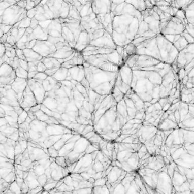
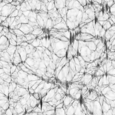
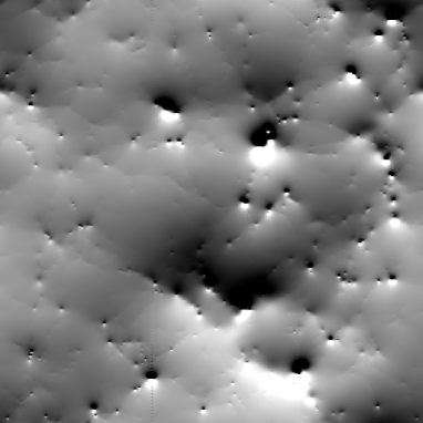
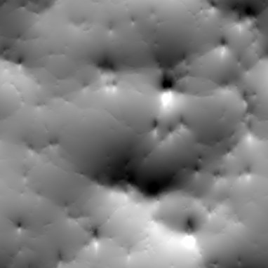
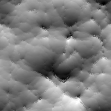
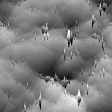
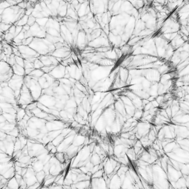
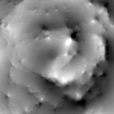
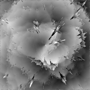
velocity field in a thin slice extracted from the simulation, both in real space and in the DOL redshift space. Despite our interpolation procedure, there are some minor discreteness artifacts left, visible on the density field. One can notice for example a few underdense regions where the initial grid pattern, distorted by large scale dynamics, is still present. Such artifacts do not show up on the smoother $z$ coordinate of the gravity field. On the other hand, this latter seems to suffer from a few aliasing defects in real space, as vertical spurious lines in the vicinity of deep potential wells. We did not bother trying to understand such aliasing effects, because they have negligible impact on the measurements. Interesting to notice here is the nice agreement between the $z$ coordinate of the velocity field and the $z$ coordinate of the gravity field in underdense regions. These regions dominate the velocity–gravity statistics, since we have a volume weighted approach. Note the particular features in the velocity field associated to the filaments in the density distribution, as well as the ‘fingers of God’ (FOG) in redshift space. These FOG, which are mainly associated to the dark matter halos, are expected to induce some particular properties on redshift space statistics:

• First, and this is a straightforward consequence of passing from real space to redshift space, there is, on the velocity field, an ‘inversion’ effect inside FOG. In other words, inside a finger of God, the variations of the velocity field are opposite to what happens in its nearby environment. This can be explained in the following way. Inside a halo, which can be, in real space, considered as a point-like structure in first approximation, there are particles with positive velocities and particles with negative velocities. Assume, to simplify, that this halo has itself a zero center of mass velocity. It will, in redshift space, look like an elongated structure. Particles in this structure that have positive $z$ velocity will be above the center of mass, and particles with negative velocity will be below the center of mass. As a result, one expects, for the $z$ coordinate of the velocity, the finger of God corresponding to this halo to have positive velocities (towards light color on bottom right panel of Fig. 1) above the center of the halo and to have negative velocities (towards dark color) below the center of the halo. This is indeed what we can observe. However, in the nearby environment of the halo, the situation is somewhat opposite. Indeed, the halo is expected to lie in a filament, which itself represents a local potential well. If this well is not too strong to induce shell-crossing while passing from real to redshift space, the general trend of the velocity field is not modified, compared to real space: negative sign (towards dark color) above the filament, positive sign below it. If the filament corresponds to a sufficiently deep potential well such that shell crossing occurs, then the same effect than for FOG is expected, as can be noticed on the bottom right panel of Fig. 1 for the largest filaments.

• Second, due to the FOG stretching, halos are more elongated in redshift space, and a natural consequence is that the corresponding potential well is less deep. That is why the $z$ coordinate of the gravitational force is less contrasted in the middle right panel of Fig. 1 than in the middle left one.

Still, we can see that both in real and in redshift space, the velocity–gravity relation is going to be in quite good agreement with expectation from linear theory. Indeed and again, our measurements are volume weighted, dominated by underdense regions. The color scale on four bottom panels of Fig. 1 has been chosen such that if linear theory applies, the same color pattern should be found for the gravity and velocity field, which is the case at first glimpse, except in the densest regions, corresponding to halos or rich filaments.

Finally, similarly as the right column of panels of Fig. 1, Fig. 2 displays the density, the gravity field and the velocity field in redshift space, but without using the DOL. If one now takes into account the radial nature of the projection, it is clear that the conclusions of the previous discussion remain unchanged, at least at the qualitative level.

4.3.2 Quantitative comparison in real space

Figure 3 shows in grey scale the measured joint probability

Figure 3: The velocity–gravity relation in real space as a scatter plot, compared to theoretical prediction in the linear regime (thick diagonal line), as measured from sample (i) extracted from the simulation using the $z$ coordinate of each field. The color scale is defined as follows: the darkest area is encompassed by a 68 percent isocontour (eq. 52), corresponding approximately to a 1.5$\sigma$ contour in the Gaussian case. Then, lower isocontours, corresponding to lighter color, scale logarithmically, which emphasizes the tails of the PDF. The two upper panels correspond to the raw data interpolated on the grid with the SPH-like interpolation detailed in § 4.1, while in the bottom panel, an additional Gaussian smoothing with kernel of a fixed size $\ell=10h^{-1}$ Mpc was performed. The smoothing scale is indicated on three panels (in the two top panels, it corresponds to the mesh element size). In the top panel, predictions of velocity–gravity relation according to the spherical top hat model are displayed as solid curves. As discussed in detail in the text, these curves help to understand why the linear prediction still represents the most prominent feature of the relation, even in the highly nonlinear regime, while the tails due to nonlinear dynamics induce a ‘propeller’ shape of the scatter plot, as already noticed by Cieciela̧g et al. (2003). Such a propeller shape results in a bias on the measurement of the slope by using directly second-order moments of the bivariate PDF. This is demonstrated by plotting on middle (and bottom) panel the dotted line which gives the estimated slope from the ratio $\sqrt{\langle g_{z}^{2}\rangle/\langle v_{z}^{2}\rangle}$. This dotted line should be compared to the thick solid line. The dashed lines correspond to slopes obtained by the conditional averages $\langle g_{z}^{2}\rangle/\langle g_{z}v_{z}\rangle$ and $\langle g_{z}v_{z}\rangle/\langle v_{z}^{2}\rangle$. In the middle panel these slopes are significantly different, consistent with significant amount of the scatter in the relation, due to nonlinear effects. In the middle panel, also the $1.5\sigma$ contour expected in the Gaussian case is shown.

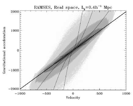
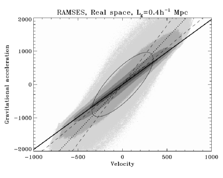
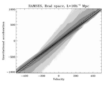
distribution function (PDF) of the $z$ coordinate of gravity and velocity fields extracted from the real space sample (i). The striking result is that the regions of the best likelihood (larger values of the PDF, darker places) match very well the prediction given by linear theory (thick solid line), even in the highly non-linear regime (upper panel). This remarkable property is mainly related to our volume-weighted approach: results are mainly influenced by underdense regions, which are weakly evolved from the dynamical point of view and are expected to match well linear theory predictions. This, and the ‘propeller’ shape of the bivariate PDF, can be understood in more detail by using the spherical top-hat model as a proxy of nonlinear dynamics. In that case, up to shell crossing, the velocity–gravity relation reads approximately

$$g\simeq\frac{R}{3}\left[1-\left(1-2\frac{v}{\beta R}\right)^{3/2}\right]$$ (51)

(this can be easily derived from Bernardeau 1992; 1994), where $R$ is the distance from the center of a top-hat fluctuation (in $\rm km\cdot s^{-1}$). This equation is valid inside the fluctuation, which can be overdense (negative $v$) or underdense (positive $v$). One can then imagine, to simplify, the density field as a patchwork of spherical fluctuations, which correspond to a set of curves given by Equation (51), as shown in the top panel of Fig. 3. Note here that we should, for the picture to be correct, take into account the fact that we are using only the $z$ coordinate of the fields, $g_{z}=g\cos\theta$ and $v_{z}=v\cos\theta$, where $\theta$ is the angle between the $z$-axis and the radial vector ${\bf R}$. In the top panel of Fig. 3, we consider the cases $R\cos\theta=\pm 10,\ \pm 100,\ \pm 1000,\ \pm 3000$ km/s. Each curve has a stopping point corresponding to the maximum possible value of $v$, $v_{\rm max}=\beta R/2$, which reflects the fact that there is an expected upper bound for the expansion speed of voids. This property excludes the upper left and lower right quadrants of the velocity–gravity diagram to be populated too far from linear theory prediction. On the other hand, overdense fluctuations tend to populate the upper right and the lower left quadrants, above and below linear theory prediction, respectively. Furthermore, since the low-$v$ regime converges to linear theory, all the curves corresponding to Equation (51) superpose in that regime, creating a ‘caustic’ of best likelihood nearby the maximum of the joint PDF, explaining the very good agreement with linear expectation in that region. As a result, we now understand, thanks to the spherical top-hat model, both the ‘propeller’ shape of the bivariate PDF, as well as the remarkable agreement with linear theory prediction nearby its maximum, even in the highly non-linear regime (see also Cieciela̧g et al., 2003). The arguments developed here are oversimplified, but capture the main features of the dynamics of the large scale structures prior to shell crossing in real space. Beyond shell crossing, there is a mixing effect that tends to decorrelate velocity from gravity, implying a widening of the bivariate PDF and even larger tails in the upper right and the lower left quadrants. However such an effect does not affect significantly the region of best likelihood.

A straightforward consequence of the above discussion is that the joint PDF of gravity and velocity is substantially non Gaussian due to non-linear contributions in the dynamics, as supported by the examination on middle panel of Fig. 3 of the 1.5$\sigma$ elliptic isocontour of the Gaussian distribution with the same second order moments as the measured PDF. As a result, the direct measurement of $\beta$ parameter from the moments of the joint PDF using linear theory predictions is biased to lower values, due the propeller shape of the PDF. This is illustrated on middle panel of Fig. 3 by the dotted line, which gives the velocity–gravity relation obtained from the second order moments of the PDF, $\sqrt{\langle g_{z}^{2}\rangle/\langle v_{z}^{2}\rangle}$, while the two dashed lines correspond to the conditional averages $\langle g_{z}^{2}\rangle/\langle g_{z}v_{z}\rangle$ and $\langle g_{z}v_{z}\rangle/\langle v_{z}^{2}\rangle$. In the linear regime, let us remind from § 2 that these three quantities should be equal. Due to non-linear effects, the relation between gravity and velocity is not deterministic anymore, $\langle g_{z}^{2}\rangle/\langle g_{z}v_{z}\rangle>\sqrt{\langle g_{z}^{2}\rangle/\langle v_{z}^{2}\rangle}>\langle g_{z}v_{z}\rangle/\langle v_{z}^{2}\rangle$, and $\beta$ is underestimated, leading to an effective bias or an underestimated value of $\Omega$, as shown in Table 1. Note, as expected, that additional smoothing of the fields with a Gaussian window of radius 10 $h^{-1}$ Mpc helps to reduce non Gaussian features as well as this effective bias, and makes the overall relation between gravity and velocity tighter.

However, Fig. 3 appeals for a more sophisticated way to measure the velocity–gravity relation than simply using directly the moments of the joint PDF. Since the region around the maximum seems to agree rather well with the linear prediction, this suggests to estimate the moments from the PDF only within that region. To perform such an exercise, we selected the 68-percent PDF isocontour, ${\cal P}_{68}$, such that

$$\int_{{\cal P}(g,v)>{\cal P}_{68}}dg\ dv\ {\cal P}(g,v)=0.68.$$ (52)

This corresponds roughly to a $1.5\sigma$ contour in the Gaussian case. The PDF is then set to zero outside the contour of best likelihood. From this truncated PDF, the moments are estimated again, leading to a much better estimate of $\Omega$, agreeing at the few percent level with the true value, as shown in Table 1, regardless whether additional Gaussian smoothing with a $10\ h^{-1}$ Mpc size window is performed on the fields, or not. Furthermore, the estimators $\sqrt{\langle g_{z}^{2}\rangle/\langle v_{z}^{2}\rangle}$, $\langle g_{z}^{2}\rangle/\langle g_{z}v_{z}\rangle$ and $\langle g_{z}v_{z}\rangle/\langle v_{z}^{2}\rangle$ differ now only slightly from each other, reflecting the narrowness of the region of best likelihood around the linear expectation.

4.3.3 Quantitative comparison in redshift space

Figure 4 is similar to Fig. 3, but shows the results obtained from

Figure 4: The velocity–gravity relation in distant observer redshift space as measured from sample (ii) extracted from the simulation, using the $z$ coordinate of the fields. The color scaling is the same as in Fig. 3. Again the match between the most likely part of the bivariate PDF (darkest region) and the prediction from linear theory (thick solid line) is close to perfect. The dotted line gives the slope obtained directly from the ratio $\sqrt{\langle g_{z}^{2}\rangle/\langle v_{z}^{2}\rangle}$. The left panel which corresponds to minimum amount of smoothing can be compared to the two upper panels of Fig. 3. The differences with real space results are explained by the arrows: large scale redshift distortion (LSRD) increases the effective slope of the velocity–gravity relation, while the finger of God (FOG) effect moves points from the upper right down to the left, and points from the lower left up to the right, creating two additional tails of the PDF. As discussed in the text, this is due to the inversion of the signature of velocity happening in fingers of God as seen in the bottom right panel of Fig. 1, and to the effective smoothing of gravitational potential due to the extended nature of the FOG. When smoothing with a Gaussian window of radius $\ell=10\;h^{-1}\rm Mpc$ is performed, these two tails move back to the upper right and the lower left of the panel: one recovers the propeller shape obtained in real space. However, its effect is more pronounced, because there is still some remnant of the anti-diagonal effect, depending on the level of smoothing.

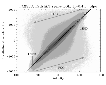
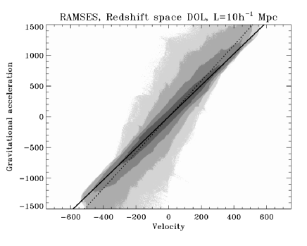
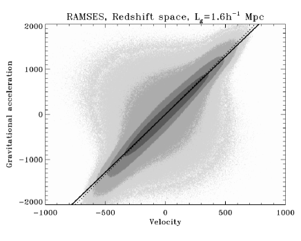
the sample (ii), in the DOL redshift space. The same striking result obtained as in real space holds: the region of maximum likelihood agrees very well with the linear theory prediction, which gives a velocity–gravity slope larger than in real space because of the enhancement of large scale density contrasts due to projection in redshift space (symbol LSRD – Large Scale Redshift Distortion – on the left panel).

However, there is on Fig. 4 a noticeable new feature on the PDF visible on left panel, in addition to the propeller shape: the joint PDF seems now to present tails in the directions orthogonal to the maximum likelihood domain. Note that these tails tend to disappear with smoothing which then makes the bivariate PDF look very much like the real space one.

This new feature is due to the finger-of-God effects already discussed at length in § 4.3.1. These effects have mainly two consequences: first, the gravitational potential is less contrasted at small scales due to the elongated nature of fingers of God, which tend to reduce the amplitude of the gravitational acceleration inside them and in their neighborhood. Second, there is an inversion effect which changes the sign of the velocity. The consequence is that some points that were, in real space, on the upper right quadrant are moved to the upper left quadrant as indicated by the arrow on the left panel of Fig. 4. These points create a tail on the upper left quadrant; similarly some points that lied in the lower left quadrant contribute to the tail on the lower right quadrant.

In fact, in the same way as we did in real space, the results obtained in redshift space can again be interpreted qualitatively using the top hat spherical collapse model, as detailed in Appendix A. Note interestingly that in the linear regime, the top hat model gives

$$\frac{g_{z}}{v_{z}}=\frac{1}{\beta}\left(1+\frac{\beta}{3}\right),$$ (53)

a value significantly smaller than what is obtained from Eqs. (24), (25) and (26): equation (53) gives $g_{z}/v_{z}\simeq 2.3$ instead of $2.6$. This disagreement with the statistical expectation from linear theory is explained in Appendix A. However, despite the limitations of the spherical top hat model, the arguments developed previously in the real space case to explain why the linear regime dominates the most likely part of the joint PDF still hold.

Thanks to finger-of-God effects, if no additional smoothing is applied to the interpolated fields, the measured joint PDF is now much more symmetric about the linear prediction than in real space. As a consequence, the slope obtained from the direct measurement of $\sqrt{\langle g_{z}^{2}\rangle/\langle v_{z}^{2}\rangle}$ (dotted line on left panel of Fig. 4) agrees now well with linear theory, while we still have $\langle g_{z}^{2}\rangle/\langle g_{z}v_{z}\rangle>\sqrt{\langle g_{z}^{2}\rangle/\langle v_{z}^{2}\rangle}>\langle g_{z}v_{z}\rangle/\langle v_{z}^{2}\rangle$. However, when an additional Gaussian smoothing is performed, the fingers of God tend to be diluted. This implies on Fig. 4 a clockwise rotation of the upper left tail to the upper right and of the lower right tail to the lower left. As a consequence, with our $10\ h^{-1}$ Mpc scale Gaussian smoothing, one converges to similar behavior as obtained in real space, with the propeller effect significantly biasing the overall slope, implying again that $\Omega$ is biased low. This bias is more pronounced in redshift space than in real space, because there is still some remnant of the anti-diagonal effect, depending on the level of smoothing. Of course, smoothing at larger scales would make the agreement with linear theory prediction better again.

To reduce the bias, one can play again the exercise of measuring the slope of the velocity–gravity relation by selecting the region of best likelihood, as in Equation (52). The agreement with linear theory prediction is improved as expected, and the corresponding measured value of $\Omega$ matches very well the real value as illustrated by Table 1. However, additional smoothing tends to mix the nonlinear finger of God effects with linear features, contaminating the region of best likelihood. As a result, the measured value of $\Omega$ is slightly biased to lower values ($0.28$ instead of $0.3$) and changing the likelihood contour selection does not improve significantly the results. This mixing effect brought by smoothing suggests that in fact it might be not so wise to perform additional smoothing of the interpolated fields. Even though smoothing at sufficiently large scales brings better overall agreement with linear theory, it makes the measurements much more sensitive to finite volume and edge effects and it is furthermore not needed here since linear theory regime always dominates the region of best likelihood. Besides, we showed in § 3 that smoothing was making the DOL approximation worse.

Figure 5 is exactly the same as Fig. 4, but the measurements

Figure 5: Same as in Fig. 4, but for the sample (iii) which does not assume that the observer is (infinitely) distant. Although the general behavior is exactly the same as in Fig. 4, several explainable differences can be noticed. The measurement is more noisy and the apparent width of the bivariate distribution is smaller than on Fig. 4. This is mainly related to the fact that the sampled volume covers only 18 percent of the simulation box. Still, the most likely part of the PDF fits very well the slope predicted by linear theory in the infinite remote observer approximation, lending credence to our simplified approach.

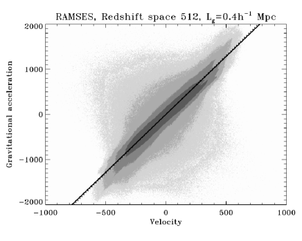
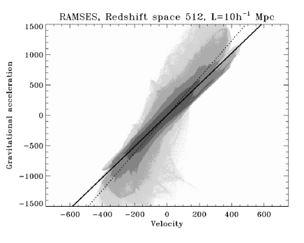
are now performed in sample (iii), without assuming that the observer is (infinitely) remote. Qualitatively, all the conclusions derived from the analysis of Fig. 4 still hold. The main difference is that the measurements are more noisy due to the size of the sampled volume, now 5 times smaller. Therefore, the recovered value of $\Omega$ from the measurements of the moments in the region of best likelihood of the joint PDF of the unsmoothed fields is good only at the ten percent level ($\Omega=0.33$ instead of $0.3$, see Table 1). At this level of accuracy, we find that the linear prediction, which was derived in the approximation of DOL, agrees well with the measurements. To improve the quality of this comparison, Figure 6 gives the same scatter plots as in Fig. 5,

Figure 6: Same as in Fig. 5, but we now consider sample (iv), where 125 different observer positions are located on a regular grid in the simulation box and where the interpolated field is computed only on a $128^{3}$ grid. As expected, the resulting bivariate PDF is smoother than in Fig. 5, since the simulation volume is now fully sampled by all these observer positions. Note the significant asymmetry of the tails of the bivariate PDF around the major axis of the maximum likelihood region. This is an expected consequence of edge effects. Indeed, while performing redshift space projection to construct a spherical catalog of finite radius $R_{\rm max}$, the galaxies near the edge of the catalog with positive radial velocity and radial position $r<R_{\rm max}$ tend to get outside the sample. On the other hand, galaxies near the edge of the catalog with negative radial velocity and radial position $r>R_{\rm max}$ tend to get inside the catalog. As a result one expects more galaxies with negative radial velocities than with positive ones, hence the asymmetry of the PDF. This effect mainly affects fingers of God, so the anti-diagonal tails of the bivariate PDF. Importantly, this effect does not affect too much the region of best likelihood.

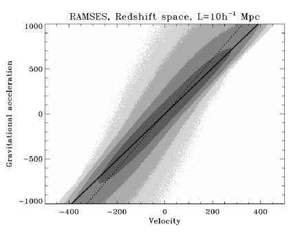
but for sample (iv), i.e. after co-adding the contributions of 125 different observers. The value of $\Omega$ derived from the best likelihood region of left panel of Fig. 6 agrees now at a few percent level with the true value of $\Omega$ (the estimated value is $0.294$, see Table 1), showing that the distant observer limit is an approximation good enough for deriving the linear prediction. Note again the bias to lower values ($0.262$) on the measured value of $\Omega$ brought by additional Gaussian smoothing with a 10 $h^{-1}\,\hbox{Mpc}$ Gaussian window. This bias is more pronounced than in the DOL sample (ii), and this is certainly at least partly due to the fact that, as discussed in § 3, deviations from the DOL limit are not negligible anymore for such a smoothing scale, given the sample depth, and they add to the mixing between linear and nonlinear features discussed above. It could also come partly from the edge effect discussed in caption of Fig. 6.

The dispersion among the 125 different observers leads to a typical error on $\Omega$ of the order of $0.04$, suggesting that the errors related to the choice of the position of the observer – which probes the space of configurations for the ${\bf s}={\bf 0}$ singularity discussed in § 3 – are of the order of 10 percent for our $R=70\ h^{-1}\,\hbox{Mpc}$ radius catalog. These errors include cosmic variance effects, but these latter are probably underestimated because our spherical redshift samples represent a rather significant fraction of the total simulation volume.

Nevertheless these measurements illustrate the relative robustness in that respect of our velocity–gravity estimator to derive $\Omega$ from a large-scale galaxy survey. However, we reiterate that, as already mentioned in beginning of § 4.1, the volume used to compute gravity field should be significantly larger than the actual volume used to perform the velocity–gravity comparison. The present analyses suppose it is the case as indeed achieved by most recent three dimensional galaxy catalogs such as the 2MRS, for which the median redshift corresponds to a half-depth of $\simeq 60\,h^{-1}$ Mpc (Erdo$\breve{\rm g}$du et al. 2006).

4.3.4 Effects of dilution

Up to now, we have measured the velocity–gravity relation in very rich catalogs, where the number of objects was so large that discreteness effects could be considered as negligible. In real galaxy catalogs, the number of objects is much smaller, particularly when tracers of the velocity field are taken at concern. Before addressing the issue of biasing between the galaxy distribution and the dark matter distribution, we therefore examine pure discreteness effects, by diluting our dark matter samples. This dilution will not only bring a shot noise contribution, it will also increase the overall level of smoothing which is performed by our interpolation procedure.

To be able to quantify as accurately as possible the biases induced by discreteness in the mock “galaxy” catalogs considered in next section, we dilute randomly our $N$-body sample in two kind of subsamples (see Table 2):

Table 2: Same as Table 1, but for the dilute dark matter sub-samples, D1 and D2.

Samp.	Content	$N_{\rm rea}$	Size	$N_{\rm g}$	$N_{\rm obj}$	Measured $\Omega$ from:			Comment
						$\frac{\langle g^{2}\rangle}{\langle vg\rangle}$	$\sqrt{\frac{\langle g^{2}\rangle}{\langle v^{2}\rangle}}$	$\frac{\langle vg\rangle}{\langle v^{2}\rangle}$
(D1)	50000, real space	125	$L=200$	128	50000	0.163	0.213	0.278	$\langle$ all $\rangle$, no smoothing
						0.004	0.006	0.008	error from dispersion
						0.237	0.252	0.268	$\langle$ all $\rangle$, smoothed
						0.007	0.008	0.009	error from dispersion
						0.283	0.300	0.319	$\langle$ 1.5$\sigma$ isocontour $\rangle$, no smoothing
						0.011	0.012	0.013	error from dispersion
						0.277	0.288	0.299	$\langle$ 1.5$\sigma$ isocontour $\rangle$, smoothed
						0.012	0.013	0.013	error from dispersion
	50000, redshift space	125	$R=70$	128	$8980^{*}$	0.062	0.248	3.841	$\langle$ all $\rangle$, no smoothing
						0.025	0.027	16.11	error from dispersion
						0.100	0.184	0.378	$\langle$ all $\rangle$, smoothed
						0.027	0.022	0.118	error from dispersion
						0.227	0.264	0.309	$\langle$ 1.5$\sigma$ isocontours $\rangle$, no smoothing
						0.030	0.034	0.050	error from dispersion
						0.209	0.237	0.269	$\langle$ 1.5$\sigma$ isocontours $\rangle$, smoothed
						0.026	0.028	0.039	error from dispersion
(D2)	11000, real space	125	$L=200$	128	11000	0.192	0.250	0.326	$\langle$ all $\rangle$, no smoothing
						0.011	0.017	0.026	error from dispersion
						0.216	0.255	0.300	$\langle$ all $\rangle$, smoothed
						0.015	0.020	0.026	error from dispersion
						0.251	0.292	0.340	$\langle$ 1.5$\sigma$ isocontour $\rangle$, no smoothing
						0.023	0.027	0.033	error from dispersion
						0.249	0.281	0.318	$\langle$ 1.5$\sigma$ isocontour $\rangle$, smoothed
						0.024	0.028	0.033	error from dispersion
	11000, redshift space	125	$R=70$	128	$1976^{*}$	0.074	0.226	1.323	$\langle$ all $\rangle$, no smoothing
						0.028	0.035	1.687	error from dispersion
						0.096	0.197	0.492	$\langle$ all $\rangle$, smoothed
						0.031	0.034	0.238	error from dispersion
						0.190	0.253	0.347	$\langle$ 1.5$\sigma$ isocontours $\rangle$, no smoothing
						0.040	0.048	0.099	error from dispersion
						0.182	0.233	0.308	$\langle$ 1.5$\sigma$ isocontours $\rangle$, smoothed
						0.040	0.044	0.089	error from dispersion

(D1)

125 realizations of dark matter catalogs involving 50000 points, similarly as for the mock with mass thresholding $M_{\rm th}=5.10^{11}\ M_{\odot}$ used in § 4.4;

(D2)

125 realizations of dark matter catalog involving 11000 points, similarly as for the mock catalogs with mass thresholding $M_{\rm th}=4.10^{12}\ M_{\odot}$ used in § 4.4.

We perform exactly the same measurements in these dilute catalogs than in sample (i) (in real space, except that we use $128^{3}$ grids for interpolating the fields and we have 125 different realizations) and in samples (iv) (in redshift space). In the latter case, note that the observer position in the simulation cube is different for each realization, chosen exactly to be on a regular patter covering the full simulation volume as in samples (iv).

Figure 7: Similarly as in Fig. 3, but for the 125 realizations of diluted samples D1 (upper panels) and D2 (lower panels). the left panels correspond to the raw interpolated fields on a $128^{3}$ grid, while for the right panels, a smoothing with a Gaussian window of size $\ell=10\ h^{-1}$ Mpc was performed prior to the measurements. Since the samples are now more diluted, the adaptive interpolating kernel is of much larger size, which decreases considerably nonlinear tails: the propeller shape of the PDF is less apparent but it still affects the measurements: the slope of the dotted line is larger than the linear expectation given by the thick solid line.

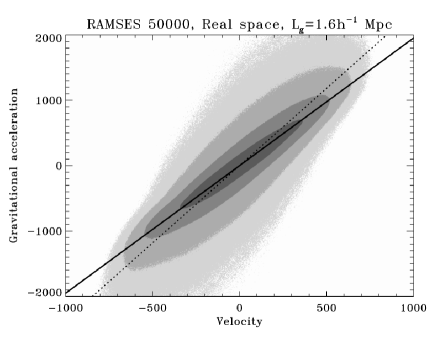
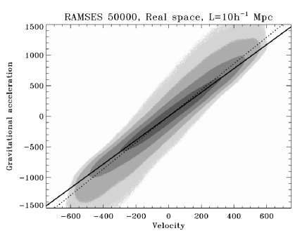
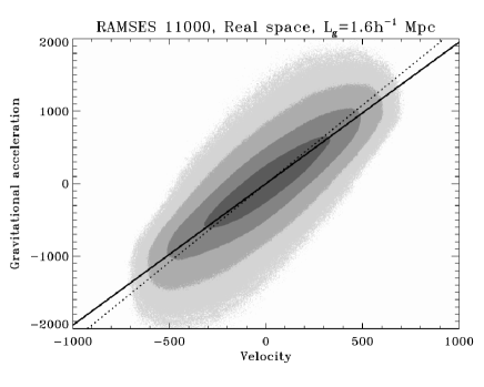
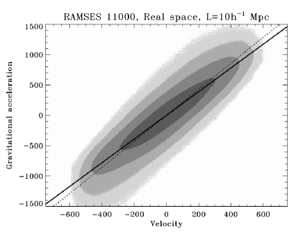
The results are summarized in Table 2 and illustrated by Figs. 7 and 8. We first discuss real space measurements using the second order moments of the full PDF and compare the values obtained for $\Omega$ to those from the undiluted sample (i), given in Table 1. Note that this sample uses a $512^{3}$ grid for the interpolation instead of the $128^{3}$ one for samples D1 and D2. Using a $128^{3}$ resolution grid increases the measured value of $\Omega$ in first line of Table 1 from $0.157$ to $0.178$. Taking that fact into account, we notice that, due to the dilute nature of the samples, our interpolation procedure uses an adaptive kernel of larger size: as shown by Fig. 7, this makes the fields more linear, closer to the Gaussian limit, and decreases the level of effective bias brought by the “propeller” shape of the bivariate PDF. As a result, prior to additional smoothing with a Gaussian window of size $\ell=10\ h^{-1}$ Mpc, the measured $\Omega$ is larger for the dilute samples than for the full one, and the convergence with linear theory prediction improves with level of dilution. The mean inter-particle distance in the sparser sample is of the order of $\lambda=9\ h^{-1}$ Mpc, slightly lower than the size of the post-processing Gaussian smoothing kernel. One thus expects rough agreement between full sample and samples D1 and D2 after smoothing with such a window, which is approximately the case. Furthermore, the measured value of $\Omega$ in D2 is not very sensitive to whether additional smoothing is performed or not, since $\lambda\simeq\ell$.

Still examining real space measurements, we now consider the values of $\Omega$ measured from second order moments of the PDF, but using only the region of best likelihood, Eq. (52), similarly as in previous paragraph. As expected, the effective bias due to nonlinear contributions (or propeller effects) is tremendously reduced, and one recovers a value of $\Omega$ compatible with the true value, given the errorbars. These latter, which estimate pure shot noise, are of the order of 4 and 10% for D1 and D2 respectively. As for the full sample, this result stands also when additional smoothing is applied to the data, although one can notice a slight bias to lower values of $\Omega$.

We now turn to redshift space measurements and first consider the measured value of $\Omega$ using the second

Figure 8: Similarly as in Fig. 6, but for the diluted samples D1 (upper panels) and D2 (lower panels).

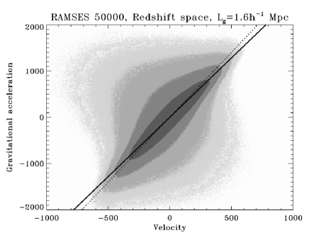
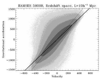
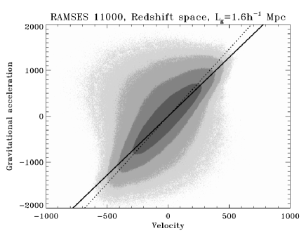
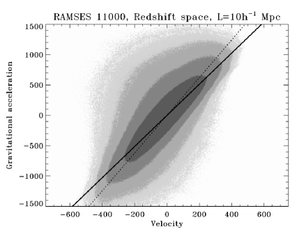
order moments of the full PDF. The results obtained in previous section still hold (compare Table 1 to Table 2), except that the measurements performed before additional Gaussian smoothing give a lower value of $\Omega$, $0.248$ for D1 and $0.226$ for D2: the low bias effect on $\Omega$ gets worse with dilution, since the larger size of the adaptive kernel tends to reduce the effect of fingers of God: as noticed previously, finger-of-God effects help to reduce the asymmetry brought by the “propeller”, the main source of the low bias on $\Omega$. Additional Gaussian smoothing with a window of size $\ell=10\ h^{-1}$ Mpc improves the convergence between D1, D2 and the full sample, as expected, but induces a highly underestimated value of $\Omega\sim 0.2$, because of the propeller effects which are then prominent. These arguments are supported by examination of Fig. 8. Note that the asymmetry of the tails of the bivariate PDF around the major axis of the maximum likelihood region, already observed and explained in Fig. 6, is now more pronounced, at least from the visual point of view.

Measurements are improved while selecting the region of best likelihood, but not as well as in the real space case or in the redshift space case with full sampling: at best, $\Omega$ is underestimated by about 12 percent. Additional smoothing or passing from D1 to D2 expectingly increases the bias. This underestimate comes again from the fact that the adaptive interpolating kernel is now of much larger extension than for the full particles sample, which induces biases comparable to what was observed for the full samples with additional smoothing (§ 4.3.3).

Note that it is possible to reduce the effective bias observed on $\Omega$ by narrowing the region of best likelihood at the price of an increase of the errors. For instance, taking a 38 percent confidence region enclosed by a $\simeq 1\sigma$ isocontour gives $\Omega=0.285$ and $\Omega=0.273$ for D1 and D2, respectively. Our procedure for measuring $\Omega$ can thus certainly be improved with a more sophisticated treatment of the region of best likelihood. For instance, a way to extract in an unbiased way the parameter $\Omega$ from the data could consist in measuring the local slope of the skeleton of the surface representing the bivariate PDF (see Novikov, Colombi & Doré, 2006) after appropriate (adaptive) smoothing of the velocity–gravity scatter plot. This is left for future work; in what follows, we shall still use for the sake of simplicity our $1.5\sigma$ likelihood contour technique, while staying aware of the bias brought by dilution.

4.4 Measurements on simple mock “galaxy” catalogs

To estimate in a sufficiently realistic way how biasing affects the results on the velocity–gravity relation, we extracted from the simulation four “galaxy” catalogs, corresponding to two methods of treating dark matter halos. In the first method, we consider each dark matter halo as a galaxy. In the second method, we consider each substructure present in dark matter halos as a galaxy. The details are given in § 4.4.1. For each kind of “galaxy catalogs”, two level of biasing are considered, corresponding to small and large threshold on the dark matter (sub)-halos masses, $M>5.10^{11}\ M_{\odot}$ and $M>4.10^{12}\ M_{\odot}$ respectively. In all cases, each galaxy is given the same weight while density and velocity are interpolated as explained in § 4.1. This rather extreme way of treating the bias is far from being optimal: appropriate weighting could be given to each object in order to correct at least partly for the effects of the bias, as further discussed in the conclusions of this paper.

The quantitative analysis of the velocity-gravity relation is performed in § 4.4.2. The measurements are interpreted in the light of the previous paragraphs analyses, using as a guideline the large scale bias obtained from the measurement of the power-spectrum of the “galaxy” distribution.

4.4.1 The mock catalogs

To extract halos and substructures from the simulation, we use the publically available software adaptaHOP (Aubert, Pichon & Colombi, 2004). AdaptaHOP builds an ensemble of trees. Each tree corresponds to a halo which is a connected ensemble of particles with SPH density $\rho>81$. The branches of the trees are composite structures of which the connectivity is controlled by the saddle points in the particle distribution. The leaves of the trees correspond to the smallest possible substructures one can find in the simulation. From this ensemble of trees, we extract two kinds of catalogs, one where each galaxy is identified to a tree, the other one where each galaxy is identified to the leaves of the trees (if a tree has only one leaf, it means that the halo is its own single substructure). Note that velocities of these galaxies are computed as the average velocity of all the particles belonging to the corresponding (sub-)structure.

Additional mass thresholding is used to control the number of “galaxies” in the catalogs,. In final, 4 mock catalogs are obtained (see also Table 3):

Table 3: Same as Table 1, but for the “galaxy” catalogs, (v)–(viii). In the second column, it is specified if they correspond to a halo (“HAL.”) or a substructure catalog (“SUBS.”) and what mass threshold was used to select the dark matter (sub-)structures. The values of $\Omega$ displayed in columns seven to nine are obtained from the measured $\beta$ assuming linear theory predictions with no bias. As a guidance to understand the results, we show in the second column of the table the measured value of the bias $b$ at the simulation box size scale (using the power-spectrum of the interpolated density), as well as $\Omega_{\rm eff}=\Omega/b^{9/5}$, the expected value of $\Omega$ from the measured $\beta$ if unity bias is assumed.

Samp.	Content	$N_{\rm rea}$	Size	$N_{\rm g}$	$N_{\rm obj}$	Measured $\Omega$ from:			Comment
						$\frac{\langle g^{2}\rangle}{\langle vg\rangle}$	$\sqrt{\frac{\langle g^{2}\rangle}{\langle v^{2}\rangle}}$	$\frac{\langle vg\rangle}{\langle v^{2}\rangle}$
(v)	HAL. $>5{\rm e}11M_{\odot}$, real space	1	$L=200$	128	43482	0.304	0.375	0.464	all, no smoothing
	$b=0.80$, $\Omega_{\rm eff}=0.45$					0.330	0.379	0.435	all, smoothed
						0.318	0.368	0.426	1.5$\sigma$ isocontour, no smoothing
						0.329	0.370	0.415	1.5$\sigma$ isocontour, smoothed
	HAL. $>5{\rm e}11M_{\odot}$, red. space	125	$R=70$	128	$7874^{*}$	0.208	0.313	0.487	$\langle$ all $\rangle$, no smoothing
	$b=0.80$, $\Omega_{\rm eff}=0.45$					0.033	0.035	0.089	error from dispersion
						0.259	0.312	0.378	$\langle$ all $\rangle$, smoothed
						0.035	0.039	0.055	error from dispersion
						0.311	0.360	0.419	$\langle$ 1.5$\sigma$ isocontours $\rangle$, no smoothing
						0.054	0.063	0.082	error from dispersion
						0.310	0.345	0.385	$\langle$ 1.5$\sigma$ isocontours $\rangle$, smoothed
						0.058	0.064	0.078	error from dispersion
(vi)	HAL. $>4{\rm e}12M_{\odot}$, real space	1	$L=200$	128	11934	0.206	0.254	0.313	all, no smoothing
	$b=0.95$, $\Omega_{\rm eff}=0.33$					0.218	0.254	0.296	all, smoothed
						0.225	0.259	0.297	1.5$\sigma$ isocontour, no smoothing
						0.231	0.258	0.288	1.5$\sigma$ isocontour, smoothed
	HAL. $>4{\rm e}12M_{\odot}$, red. space	125	$R=70$	128	$2143^{*}$	0.155	0.220	0.320	$\langle$ all $\rangle$, no smoothing
	$b=0.95$, $\Omega_{\rm eff}=0.33$					0.029	0.030	0.055	error from dispersion
						0.178	0.221	0.277	$\langle$ all $\rangle$, smoothed
						0.030	0.032	0.045	error from dispersion
						0.215	0.255	0.305	$\langle$ 1.5$\sigma$ isocontours $\rangle$, no smoothing
						0.044	0.049	0.065	error from dispersion
						0.215	0.245	0.282	$\langle$ 1.5$\sigma$ isocontours $\rangle$, smoothed
						0.045	0.049	0.061	error from dispersion
(vii)	SUBS. $>5{\rm e}11M_{\odot}$, real space	1	$L=200$	128	55044	0.215	0.253	0.298	all, no smoothing
	$b=0.97$, $\Omega_{\rm eff}=0.32$					0.248	0.265	0.283	all, smoothed
						0.260	0.281	0.303	1.5$\sigma$ isocontour, no smoothing
						0.264	0.277	0.292	1.5$\sigma$ isocontour, smoothed
	SUBS. $>5{\rm e}11M_{\odot}$, red. space	125	$R=70$	128	$9886^{*}$	0.101	0.228	0.607	$\langle$ all $\rangle$, no smoothing
	$b=0.97$, $\Omega_{\rm eff}=0.32$					0.024	0.020	0.223	error from dispersion
						0.144	0.198	0.277	$\langle$ all $\rangle$, smoothed
						0.023	0.019	0.041	error from dispersion
						0.234	0.264	0.299	$\langle$ 1.5$\sigma$ isocontours $\rangle$, no smoothing
						0.030	0.035	0.045	error from dispersion
						0.224	0.244	0.267	$\langle$ 1.5$\sigma$ isocontours $\rangle$, smoothed
						0.028	0.031	0.038	error from dispersion
(viii)	SUBS. $>4{\rm e}12M_{\odot}$, real space	1	$L=200$	128	11221	0.189	0.226	0.269	all, no smoothing
	$b=1.035$, $\Omega_{\rm eff}=0.28$					0.204	0.228	0.254	all, smoothed
						0.215	0.239	0.266	1.5$\sigma$ isocontour, no smoothing
						0.218	0.236	0.255	1.5$\sigma$ isocontour, smoothed
	SUBS. $>4{\rm e}12M_{\odot}$, red. space	125	$R=70$	128	$2015^{*}$	0.102	0.176	0.327	$\langle$ all $\rangle$, no smoothing
	$b=1.035$, $\Omega_{\rm eff}=0.28$					0.024	0.020	0.082	error from dispersion
						0.123	0.170	0.241	$\langle$ all $\rangle$, smoothed
						0.023	0.021	0.040	error from dispersion
						0.178	0.211	0.251	$\langle$ 1.5$\sigma$ isocontours $\rangle$, no smoothing
						0.030	0.033	0.046	error from dispersion
						0.177	0.201	0.230	$\langle$ 1.5$\sigma$ isocontours $\rangle$, smoothed
						0.030	0.032	0.041	error from dispersion

(v)

A “halos” catalog, involving 43482 dark matter halos with masses larger than $M_{\rm th}=5.10^{11}\ M_{\odot}$;

(vi)

A “massive halos” catalog, involving 11934 dark matter halos with masses larger than $M_{\rm th}=4.10^{12}\ M_{\odot}$;

(vii)

A “sub-structures” catalog, involving 55044 dark matter sub-halos with masses larger than $M_{\rm th}=5.10^{11}\ M_{\odot}$;

(viii)

A “massive sub-structures” catalog, involving 11221 dark matter sub-halos with masses larger than $M_{\rm th}=4.10^{12}\ M_{\odot}$.

From each of these catalogs, we compute the velocity and gravity field on a $128^{3}$ grid as explained in § 4.1, in real and redshift space. In the latter case, we use 125 different observers and perform the measurements in a sphere of radius $70\,h^{-1}\,\hbox{Mpc}$ Mpc centered on the observer exactly as was done to generate the pure dark matter realizations (iv) in § 4.3.

The philosophy underlying to the making of these catalogs relies on the facts that:

(a)

dark matter substructures are reasonable tracers of galaxies (e.g. Springel et al. 2001; Weinberg et al. 2006). In that sense, one can consider the sub-structure catalogs as the most realistic. This is known to be true only to a limited extent. Indeed, sub-halos tend to be tidally disrupted while they spiral in their host halo, therefore one expects less sub-structures than galaxies in the core of dark matter halos (e.g. Diemand et al. 2004; Nagai & Kravtsov 2005). This is all the more true since we apply a mass thresholding to control the number of objects in our catalogs. However, the effect of such a depletion should be noticeable only at the smallest scales and should not affect significantly the results of the analyses at the level of accuracy reached in this paper.

(b)

dark matter halos are representative of the galaxy distribution in terms of an ensemble of structures composed of clusters, groups of galaxies and field galaxies. Therefore, if one considers the galaxy distribution from a slightly different perspective, these structures can be used as well to study the velocity–gravity relation, with the appropriate weighting. The potential advantage of such an approach is to reduce considerably the fingers of God effects discussed previously, since all the galaxies belonging to one cluster or group of galaxies are collapsed to a single point. Note that we oversimplify the analyses here by purposely giving the same weight to all the dark matter halos: this rather extreme procedure is expected to introduce quite significant (anti-)biasing effects on the gravity field determination.

4.4.2 Quantitative measurements and the effect of the bias

The results of our analyses are summarized in Table 3 and illustrated by Figs. 9 and 10.

Figure 9: The velocity–gravity relation in real space as measured in our mock “galaxy” catalogs (v)–(viii). The left column of panels corresponds to the direct SPH alike interpolation on a $128^{3}$ grid, while an additional Gaussian smoothing with a window of size $10\ h^{-1}$ Mpc was performed in the right column of panels. The informations on the catalogs are given as titles on each panel, namely, from top to bottom, halo catalog with mass thresholding $M_{\rm th}=5.10^{11}M_{\odot}$, sub-structure catalog with $M_{\rm th}=5.10^{11}M_{\odot}$, halo catalog with $M_{\rm th}=4.10^{12}M_{\odot}$ and sub-structure catalog with $M_{\rm th}=4.10^{12}M_{\odot}$. The prediction from linear theory in absence of bias is given as the solid line while the slope obtained directly from the ratio $\sqrt{\langle g_{z}^{2}\rangle/\langle v_{z}^{2}\rangle}$ is represented as a dotted line.

Figure 10: Same as in Fig. 9, but in redshift space. The scatter plots are obtained from the average of 125 observer positions disposed on a regular pattern spanning the simulation volume. As expected, finger of God effects are more prominent on the sub-structures catalogs than on the halos catalogs.

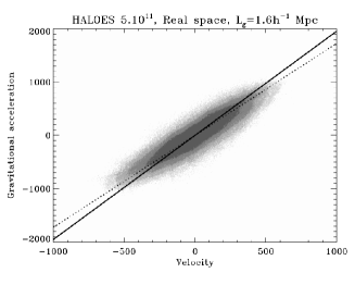
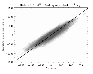
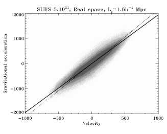
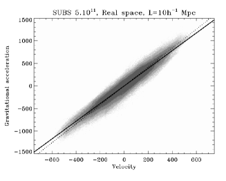
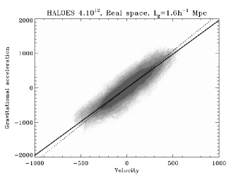
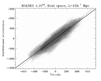
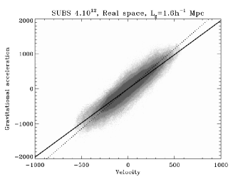
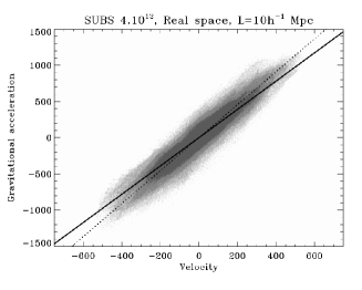
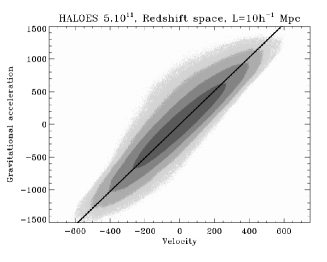
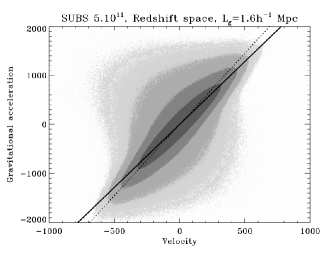
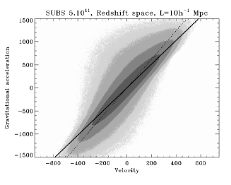
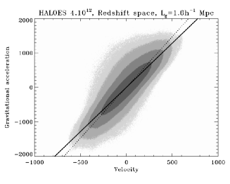
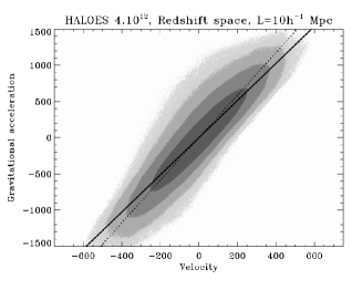
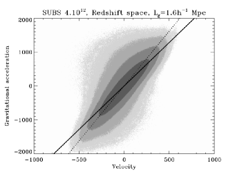
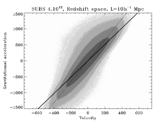
As shown in § 4.3, due to nonlinear effects, measurements based on the direct estimation of the moments of the joint probability of velocity and gravity tend to bias the estimated linear $\beta$ to lower values, both in real and redshift space. To reduce this systematic effect, we propose to consider only the region of best likelihood. Strictly speaking, this approach makes sense only if the bias between the galaxy distribution and the dark matter distribution is either inexistent or linear. The concept of a non local, scale dependent bias as experienced here complicates considerably the analyses. However, the aim is to capture the linear contribution of the dynamics, which in terms of our volume-weighted measurements is dominated by underdense regions. In these regions, the size of the adaptive kernel is large: inside the contour of best likelihood of the joint PDF, the measurements are expected to be dominated by the large scale bias, $b(k)$, with small wavenumber $k$. In that regime, the bias is in general roughly linear or close to linear. The need to actually consider the region of best likelihood of the PDF to perform the measurements is therefore furthermore justified. As a result, in what follows, only results of Table 3 obtained from selecting the region inside the $1.5\sigma$ contour of the PDF are considered. Since additional smoothing tends to introduce additional bias in the redshift space measurements, it will not be discussed either, although the results are shown in Table 3 for completeness.

We first discuss real space measurements and try to understand the effects of the bias. Sample (v) is the halo catalog with low mass threshold. This catalog is expected to present significant antibias. Indeed, if small halos, which mainly lie in moderately dense and underdense regions, trace rather well the underlying dark matter distribution, the largest ones, which are collapsed to a single point, induce a significant underestimate of the overall strength of the dark matter gravity field, resulting in the antibias effect. As shown in Table 3, the value of the bias measured at the simulation box size (using the Fourier modes at the largest scales) gives $b(k=2\pi/L)=0.8$. If one uses, as argued above, this value of $b$ as a reference, the effective value of $\Omega$ obtained from linear theory, ignoring the bias, is larger than the true one, $\Omega_{\rm eff}=\Omega/b^{9/5}=0.45$. This is to be compared to the value of $0.37$ obtained from $\sqrt{\langle g^{2}\rangle/\langle v^{2}\rangle}$. Although this latter result is significantly lower than the “expected” value, two facts have to be taken into account:

1. As an effect of non local, scale dependent biasing, the correlation between gravity and velocity field is not as tight as for the dark matter diluted sample, D1, albeit this latter contains the same number of objects. Indeed, one measures $\Omega=0.31$ and $0.42$ from $\langle g^{2}\rangle/\langle vg\rangle$ and $\langle vg\rangle/\langle v^{2}\rangle$ respectively in sample (v), while $\Omega$ was ranging between $0.28$ and $0.32$ for D1. This loss of tightness in the velocity-gravity relation obviously affects in a non trivial way the region of best likelihood.

2. Our approach for estimating the effects of the bias is rather crude and does not give account of the additional subtleties related to our adaptive smoothing procedure.

Taking these two points into account, the measurements are rather consistent with the expectations, at least at the qualitative level.

In the halo catalog (vi), small mass “galaxies” are removed, so the underdense regions are not populated anymore, leaving us with a set of more clustered objects than in sample (v), since the higher is their mass, the more significantly the halos are clustered. The consequence is that the antibias found in catalog (v) is reduced to $b(k=2\pi/L)=0.95$, resulting in an effective expected value of $\Omega_{\rm eff}=0.33$, to be compared with the value of $0.26$ obtained from the measurement of $\sqrt{\langle g^{2}\rangle/\langle v^{2}\rangle}$. Again the arguments (a) and (b) developed just above apply, leading us to conclude that this result is consistent with expectations, and similarly for the substructures catalogs: sample (vii) is the closest to the underlying dark matter distribution, with a very slight antibias of $b(k=2\pi/L)=0.97$ and $\Omega_{\rm eff}=0.32$ to be compared to $0.28$ from $\sqrt{\langle g^{2}\rangle/\langle v^{2}\rangle}$; sample (viii) presents a small positive large scale bias, with $b(k=2\pi/L)=1.035$ and $\Omega_{\rm eff}=0.28$, to be compared to $0.24$ from $\sqrt{\langle g^{2}\rangle/\langle v^{2}\rangle}$.

We can conclude here that we understand what are the various effects influencing the measurements in the mock catalogs. The general trend is that the “true” value of parameter $\beta$ (i.e. the very large scale one) seems to be underestimated by about 10 to 20 percent. We give here quotes, because such a value is not well defined. Indeed, the interpretation of the measurements is complicated by adaptive filtering, combined with a non local, scale dependent bias. But as discussed above, we really want to capture the value of $\beta$ in the linear regime limit, where the bias is expected to be roughly linear, scale independent and in fact rather close to unity, as observed in our “galaxy” catalogs. Note interestingly that the conditional moment $\langle vg\rangle/\langle v^{2}\rangle$ gives a rather good estimate of the expected value of $\beta$. Without going too far exploiting such a property, which may be specific to our catalogs, it is clear that the slopes given by the two conditional moments could be used as proxies to estimate a range of possible values for $\beta$, or in other words, errorbars. Indeed, the difference between these slopes is related to the width of the likelihood region, i.e. it estimates the tightness of the correlation between gravity and velocity as measured in the catalog. However, note that this difference does not properly give account of systematic effects discussed at length in this paper, as well as cosmic variance effects, although it is indirectly related to them.

We now turn to redshift space measurements. What matters is that they should be self-consistent with the real space ones. This is nearly the case, except again that they tend to underestimate real space measurements by up to ten percent, an effect of sparse sampling discussed in § 4.3.4, with no additional surprise. Overall, the difference between the measured value of $\Omega$ in redshift space and the “expected’, effective one, $\Omega_{\rm eff}$, is about 25 percent, with a systematic bias to lower values, as always. Obviously our mock catalogs are very peculiar in a sense that they represent quite an extreme case in the range of possibilities. And still, without any assumption on the bias, or in other words, assuming that $b$ is of the order of unity, we can determine $\Omega$ with an accuracy of the order of 30 percents without significantly strong prior. Furthermore, the quality of this estimate can certainly be improved with appropriate weighting of the galaxies. However, as discussed in the conclusion that follows, the sources of systematic errors related to the instrumental noise or to the method used to provide velocities were not considered here.

5 Conclusions

In cosmic density–velocity comparisons, since the density field is given solely in redshift space, redshift-space effects have to be accounted for. One method is to perform the analysis directly in redshift space, as proposed by ND (Nusser & Davis 1994). Another one is to reconstruct the real-space density field, but this method is complicated by the fact that redshift-space corrections require assuming a value for $\beta$. As $\beta$ is not known a priori, one is forced to reconstruct the density field for a range of values of $\beta$, which makes the real-space comparison involved, despite its apparent simplicity. In the present paper we have proposed a method that works in redshift space, but is simpler than the formalism of ND, which is based on a spherical harmonics expansion. It is essentially as simple as in real-space; the only difference is that here a directly estimated parameter is not just $\beta$, but its simple function.

This method relies on a tight correlation between cosmic gravity and cosmic velocity in redshift space. We have derived the velocity–gravity relation in redshift space and its scatter analytically, under the assumptions of the linear regime, distant observer limit (DOL) and CMB rest frame for redshift measurements. This relation has turned out to be a simple modification of the corresponding one in real space and in the linear regime. Then we have performed a dark matter $N$-body experiment to test the velocity–gravity relation both in real space and in redshift space. We also extracted mock galaxy catalogs from this data set, with rather extreme prescription for selecting “galaxies” from the dark matter distribution in order to analyze the effects of non-trivial biasing on the velocity–gravity relation. The main results are the following:

• To perform the measurements, we propose to interpolate the gravity and the velocity fields on a regular grid using a new adaptive smoothing procedure described in § 4.1. This method is close to SPH interpolation, but without the defect of having regions of space where the velocity field is undefined. Although our algorithm is expected to be less optimal than those based on Voronoi or Delaunay interpolation (e.g., Bernardeau et al. 1997; Pelupessy, Schaap & van de Weygaert 2003), it has the advantage of being simpler to implement and much faster, and can be applied to very large sets such as the $512^{3}$ sample analyzed in this paper.

• In real space, simple measurements using moments of the full joint probability distribution function (PDF) bias $\Omega$ to low values. This is due to the fact that these moments are contaminated by the tails of the PDF. These latter are influenced by nonlinear dynamics, which induces a global ‘propeller’ shape for the PDF.

• In redshift space, fingers of God (FOG) induce additional “anti-diagonal” tails to the PDF. This effect seems to somewhat compensate the bias due to the propeller shape. However this result could be coincidental and is too sensitive to the level of smoothing applied to the data. Note that in actual peculiar velocity catalogs, clusters of galaxies are in general collapsed into one point to improve the signal to noise ratio of the distance estimates. Although FOG are thus less of an issue in real data, rich filaments can still contribute to an effect similar to FOG as discussed in § 4.3.1.

• Selecting about a $1.5\sigma$ (68% confidence) region around the maximum of the joint PDF of gravity and velocity fields makes the data to match the linear theory predictions very well, both in real and in redshift space. This result stands even in the highly nonlinear regime (no additional smoothing except the adaptive interpolation on the grid). It is easily explained by the fact that our measurements are volume weighted, giving most of the statistical weight to underdense regions. Therefore, it is sufficient to exclude only the tails of the distribution to obtain unbiased estimate of $\Omega$.

• Additional smoothing does not improve the agreement with linear theory predictions: first, it is expected to increase deviations from the DOL limit; second, it makes the situation worse in the region of best likelihood, where it mixes linear contributions with nonlinear ones and biases $\beta$ to lower values, an effect which is minimized as much as possible with our adaptive smoothing procedure.

• The measurements obtained in our mock catalogs provide a value of $\beta$ in agreement with intuition, namely that large scale bias dominates if the region of best likelihood is selected. This is inherent to our volume weighted approach which gives more weight to underdense regions (see also Berlind, Narayanan & Weinberg 2001). However, due to the dilute nature of real catalogs, we expect an effective bias on $\beta$ to lower values. This bias was found to be of the order of 10–20 $\%$ for the mock samples considered in this paper. In addition, the velocity–gravity relation looses some tightness due to effects of non-local biasing between luminous and dark matter distributions. Nevertheless, our analyses show that direct measurement of $\Omega$ from real catalogs assuming no bias should give an answer accurate to about $30$ $\%$ at worse. Moreover, this error can probably be significantly improved to values as low as 10 $\%$, with the appropriate weighting of the data (purposely not performed here), as discussed below.

There are several points we did not address in our numerical analyses, and we leave them for future work:

- Noise:

through the analysis of dilute samples and mock catalogs, we addressed to some extent the effects of shot noise for realistic modern catalogs. However, we used the same catalog for velocity and gravity fields, implying that the same adaptive kernel can be used for both fields, which is not realistic. Furthermore we did not take into account the fact that there is in practice a significant relative error on galaxy distance estimates, which can be as large as 20 percent. Thus the velocity–gravity relation is certainly not expected to be as tight in real catalogs as in the samples considered in this paper. Note interestingly, though, that since the measurements are performed in redshift space, issues related to Malmquist bias (e.g., Strauss & Willick 1995) should be irrelevant, as long as the distance estimates are unbiased (just noisy).

- Incompleteness:

Another closely related issue is that the catalogs used to estimate the gravity field are incomplete. First, edge effects are expected to be significant because gravity force is of long range. The galaxy catalog used to estimate the gravity field has to be significantly deeper than the region used to perform the velocity–gravity comparison. We did not estimate in this paper how deep it has to be, not to mention the problem of obscuring by our own Galaxy. Second, the apparent density of galaxies decreases with increasing distance from the observer. In order to estimate the interpolated density field, one can, under the assumption of no bias between the galaxy distribution and the mass distribution, weight the galaxies by the inverse of the selection function, $\phi$. In the linear regime, in the absence of bias and for redshifts measured relative to the CMB rest frame, the redshift space density contrast measured that way reads (Kaiser 1987)

$$\delta_{\bf s}=\delta-\left(2+\frac{d\ln\phi}{d\ln r}\right)\frac{v}{r}-\frac{\partial v}{\partial r}.$$ (54)

Under the DOL, the second term on the right hand side of this equation drops, so the effect of the selection function disappears. However, since remote parts of the catalogs are sparser, they might be given lesser statistical weight, hence augmenting the relative contribution of this deviation from the distant observer limit.

- Better handling of the bias:

our analyses in the simple mock catalogs show that biasing affects the velocity–gravity relation in a non trivial way. However, we used the most naive prescription to compute the gravity field, giving equal weight to all galaxies. Clearly, a better description would be to assign to each galaxy a weight proportional to its supposed host halo mass, for example assuming constant mass to light ratio, $M/L$, or a more sophisticated weighting using a function $M/L=f(L)$ derived from observations or obtained from theoretical models of galaxy formation. That would allow one to correct to a large extent for the effects of biasing, at the cost of additional priors. Still, unless the galaxy catalog used to compute the gravity field is very deep, i.e. includes faint galaxies, even giving the proper mass to light ratio to each galaxy does not correct for the fact that underdense regions can be artificially underpopulated, especially far away from the observer. To tackle with that, one could add a background population of low mass objects that would give account of the missing mass in the catalog and that would act as a shielding effect on the gravity field (see, e.g., Phelps et al. 2006). Again, some strong priors are required to deal with such a background, in particular on its clustering properties and how it correlates with the population already present in the real catalog.

Note finally that while our approach presents the advantage of simplicity compared to ND (and most other methods), we do not expect it to be as accurate as of ND, since it relies on the distant observer approximation and uses in its current form adaptive smoothing, which complicates the interpretation of the results. (On the other hand, we clearly showed that the region of best likelihood of the joint velocity–gravity distribution is dominated by the linear regime prediction, even in the highly nonlinear regime, which presents a noticeable advantage.) Similarly, our method is not expected to perform as well as sophisticated reconstructions of Lagrangian nature, which try to minimize the Euler-Lagrange action (e.g., Peebles 1989; Shaya, Peebles & Tully 1995; Nusser & Branchini 2000; Phelps 2002; Phelps et al. 2006) or to solve optimal assignment problem (e.g., Croft & Gaztañaga 1997; Frisch et al. 2002; Mohayaee et al. 2003; Mohayaee & Tully 2005), although this remains to be verified.

Appendix A Spherical top-hat in redshift space

The general result in real space is

$$\frac{g_{3}}{v_{3}}=\beta^{-1}\frac{\delta}{\theta}\,,$$ (55)

where $\delta$ and $\theta$ are the real-space density contrast and velocity divergence, respectively. In redshift space, in the distant observer limit, the general result is

$$\frac{g_{3}}{v_{3}}=\frac{3}{2}C\,\beta^{-1}\left(\frac{\delta}{\theta}+\frac{\beta}{3}\right).$$ (56)

Here,

$$C=\frac{2(1-e^{2})}{e^{2}}\left[(1-e^{2})^{-1/2}-\frac{\sin^{-1}{\!e}}{e}\right],$$ (57)

eccentricity

$$e=(1-\varrho^{2})^{1/2},$$ (58)

and

$$\varrho=1-\beta\theta/3\,.$$ (59)

In the linear regime, $C=2/3$ and $\theta=\delta$. Hence,

$$\frac{g_{3}}{v_{3}}=\beta^{-1}\left(1+\frac{\beta}{3}\right).$$ (60)

We see thus that the spherical top-hat model does not give the statistical result obtained from linear theory. The reason for this is the following. In the spherical model, the velocity–gravity relation is fully deterministic, but we could also derive it calculating the relevant statistical averages. While in the linear regime, in general

$$\tilde{\delta}^{(g)}_{\bf s}({\bf k})=b(1+\beta\mu^{2})\tilde{\delta}({\bf k})\,$$ (61)

[where $\mu={\bf k}\cdot{\bf s}/(ks)$], in the spherical top-hat we have

$$\delta^{(g)}_{{\bf s},\rm TH}=b(1+\beta/3)\delta\,,$$ (62)

that immediately yields

$$\tilde{\delta}^{(g)}_{{\bf s},\rm TH}({\bf k})=b(1+\beta\langle\mu^{2}\rangle)\tilde{\delta}({\bf k})\,,$$ (63)

since $\langle\mu^{2}\rangle=1/3$. In other words, the expression for the redshift space density contrast in the top-hat model is an average of generally valid expression (61) over possible orientations of the vector ${\bf k}$. In the case of the estimator $\langle v_{\bf s}g_{\bf s}\rangle/\langle v_{\bf s}^{2}\rangle$, the average over angles yields an expression proportional to

$$\frac{\langle\mu^{2}(1+\beta\mu^{2})\rangle}{\langle\mu^{2}\rangle}=1+\beta\frac{\langle\mu^{4}\rangle}{\langle\mu^{2}\rangle}=1+\frac{3}{5}\beta\,.$$ (64)

In the top-hat model, this is modified to

$$\frac{\left\langle\mu^{2}\left(1+\beta\langle\mu^{2}\rangle\right)\right\rangle}{\left\langle\mu^{2}\right\rangle}=1+\beta\frac{\left\langle\mu^{2}\right\rangle^{2}}{\left\langle\mu^{2}\right\rangle}=1+\frac{1}{3}\beta\,.$$ (65)

Loosely speaking, the top-hat model performs a part of this average ‘too early’. So the top-hat model yields quantitatively different results from the results of a rigorous statistical calculation. However, it is sufficient for qualitative purposes, needed here. In particular, it correctly predicts that the slope of the velocity–gravity relation in redshift space gets steeper.

Turn-around in real space corresponds to extreme flatness of the pancake in redshift space. When $\theta\to\theta_{t}\equiv 3\beta^{-1}$, then $\varrho\to 0$ and $C$ tends to its maximal value, $2$. Hence,

$$\frac{g_{3}}{v_{3}}\to 3\beta^{-1}\left(\frac{\delta_{t}}{\theta_{t}}+\frac{\beta}{3}\right)\simeq 11.6\,.$$ (66)

Here, $\delta_{t}$ is related to $\theta_{t}$ by the formula of Bernardeau (1992). In fact, Bernardeau et al. (1999) invented its more accurate modification:

$$1+\delta\simeq(1+\theta/\alpha)^{\alpha},$$ (67)

where $\alpha$ is slightly greater than $3/2$. However, for our purposes $\alpha=3/2$ should be accurate enough; moreover, it better describes the evolution of voids [for this value of $\alpha$, $\delta(\theta=-1.5)=-1$]. This formula works for mildly non-linear densities.

For $\theta>3\beta^{-1}$, the structure in redshift space is inverted: velocity, and so the ratio of $g_{3}$ to $v_{3}$, changes sign. Then

$$\varrho=\beta\theta/3-1\,,$$ (68)

and

$$\frac{g_{3}}{v_{3}}=-\frac{3}{2}C\,\beta^{-1}\left(\frac{\delta}{\theta}+\frac{\beta}{3}\right).$$ (69)

For $\theta=\theta_{i}\equiv 6\beta^{-1}$ we have $\varrho=1$, so the structure in redshift space is momentarily an (inverted) sphere, hence without further effort, $C=2/3$. Therefore, then

$$\frac{g_{3}}{v_{3}}=-\beta^{-1}\left(\frac{\delta_{i}}{\theta_{i}}+\frac{\beta}{3}\right)\simeq-5.42.$$ (70)

For $\theta\gg 3\beta^{-1}$ (highly nonlinear infall), the (inverted) structure in redshift space becomes very elongated (finger of God). Then $\varrho=\beta\theta/3-1\simeq\beta\theta/3\gg 1$ and $e\simeq(1/3)\beta\theta\rm i$. After some algebra, one can show that then

$$C\to 2\frac{\ln{(\beta\theta/3)}}{(\beta\theta/3)^{2}}\,.$$ (71)

Moreover, then one cannot use formula (67), but $\delta\to(\theta/3)^{2}$ (Bilicki & Chodorowski, in preparation), hence $\delta/\theta\propto\theta$. This yields

$$-\frac{g_{3}}{v_{3}}\propto\theta^{-1}\ln{\theta}.$$ (72)

In other words, $g_{3}$ becomes very small compared to $|v_{3}|$.

References

- [1] Aubert D., Pichon C., Colombi S., 2004, MNRAS 352, 376
- [2] Bardeen J. M., Bond J. R., Kaiser N., Szalay A. S., 1986, ApJ 304, 15
- [3] Barnes J., Hut P., 1986, Nature 324, 446
- [4] Barnes J., Hut P., 1989, ApJS 70, 389
- [5] Berlind A. A., Narayanan V. K., Weinberg D., 2001, ApJ 549, 688
- [6] Bernardeau F., 1992, ApJ 390, L61
- [7] Bernardeau F., 1994, ApJ 427, 51
- [8] Bernardeau F., Chodorowski M. J., Łokas E. L., Stompor R., Kudlicki A., 1999, MNRAS 349, 543
- [9] Bernardeau F., van de Weygaert R., Hivon E., Bouchet F. R., 1997, MNRAS 290, 566
- [10] Bertschinger E., 1995, astro-ph/9506070
- [11] Bouchet F. R., Colombi S., Hivon E., Juszkiewicz R., 1995, A&A 296, 575
- [12] Branchini E., et al., 1999, MNRAS 308, 1
- [13] Chergui J., 2000, Transformées de Fourier Rapides Monoprocesseur sur NEC SX-5, publications de l’IDRIS (CNRS/IDRIS 2000), http://www.idris.fr/data/publications/fft-SX5.pdf
- [14] Cieciela̧g P., Chodorowski M. J., Kiraga M., Strauss M. A., Kudlicki A., Bouchet F. R., 2003, MNRAS 339, 641
- [15] da Costa L. N., Bernardi M., Alonso M. V., Wegner G., Willmar C. N. A., Pellegrini P. S., Rité C., Maia M. A. G., 2000, AJ 120, 95
- [16] Croft R. A., Gaztañaga E., 1997, MNRAS 285, 793
- [17] Davis M., Nusser A., Willick J. A., 1996, ApJ 473, 22
- [18] Dekel A., Bertschinger E., Yahil A., Strauss M. A., Davis M., Huchra J. P., 1993, ApJ 412, 1
- [19] Diemand J., Moore B., Stadel J., 2004, MNRAS 352, 535
- [20] Eisenstein D. J., Hu W., 1998, ApJ 496, 605
- [21] Erdodu P., et al., 2006, MNRAS 368, 1515
- [22] Frisch U., Matarrese S., Mohayaee R., Sobolevski A., 2002, Nature 417, 260
- [23] Kaiser N., 1987, MNRAS 227, 1
- [24] Kaiser N., Efstathiou G., Ellis R., Frenk C., Lawrence A., Rowan-Robinson M., Saunders W., 1991, MNRAS 252, 1
- [25] Kaiser N., Lahav O., 1988, In Large Scale Motions in the Universe, Proceedings of the Vatican Study Week, G. Coyne & V. C. Rubin, Eds. (Princeton University Press 1988), p. 339
- [26] Kaiser N., Stebbins A., 1991, in Large-Scale Structure and Peculiar Motions in the Universe, ASP Conferences Series, Vol. 15, D. W. Latham & L. N. da Costa, Eds., p. 111
- [27] Kudlicki A., Plewa T., Różyczka M., 1996, Acta A. 46, 297
- [28] Kudlicki A., Chodorowski M. J., Plewa T., Różyczka M., 2000, MNRAS 316, 464
- [29] Masters K. L., Springob C. M., Haynes M. P., Giovanelli R., Huchra J. P., 2005, American Astronomical Society Meeting 207, 170.01
- [30] Mohayaee R., Frisch U., Matarese S., Sobolevski A., 2003, A&A 406, 393
- [31] Mohayaee R., Tully R. B., 2005, ApJ 635, L113
- [32] Monaghan J. J., 1992, ARA&A 30, 543
- [33] Moutarde F., Alimi J.-M., Bouchet F.R., Pellat R., Ramani A., 1991, ApJ 382, 377
- [34] Nagai D., Kravtsov A. V., 2005, ApJ 618, 557
- [35] Novikov D., Colombi S., Doré O, 2006, MNRAS 366, 1201
- [36] Nusser A., Branchini E., 2000, MNRAS 313, 587
- [37] Nusser A., Davis M., 1994, ApJ 421, L1 (ND)
- [38] Peebles P. J. E., 1980, The Large-Scale Structure of the Universe (Princeton University Press, 1980)
- [39] Peebles P. J. E., 1989, ApJ 344, L53
- [40] Pelupessy F. I., Schaap W. E., van de Weygaert R., 2003, A&A 403, 389
- [41] Phelps S. D., 2002, ApJ 575, 1
- [42] Phelps S. D., Desjacques V., Nusser A., Shaya E. J., 2006, MNRAS 370, 1361
- [43] Saunders W., et al., 2000, MNRAS 317, 55
- [44] Shaya E. J., Peebles P. J. E., Tully R. B., 1995, ApJ 454, 15
- [45] Sigad Y., Eldar A., Dekel A., Strauss M. A., Yahil A., 1998, ApJ 495, 516
- [46] Springel V., White S. D. M., Tormen G., Kauffmann G., 2001, MNRAS 328, 726
- [47] Strauss M. A., Willick J. A., 1995, PhR 261, 271
- [48] Teuler J.-M., 1999, JMFFT: Emulation des Transformees de Fourier CRAY (CNRS/IDRIS 1999), http://www.idris.fr/data/publications/JMFFT/
- [49] Teyssier, R., 2002, A&A 385, 337
- [50] Weinberg D. H., Colombi S., Davé R., Katz N., 2006, submitted to ApJ (astro-ph//0604393)
- [51] Willick J. A., Courteau S., Faber S. M., Burstein D., Dekel A., Strauss M. A., 1997, ApJS 109, 333
- [52] Willick J. A., Strauss M. A., 1998, ApJ 507, 64
- [53] Yahil A., Strauss M. A., Huchra J. P., 1991, ApJ 372, 380
- [54] Zel’dovich Ya. B., 1970, A&A 5, 84