NON-GAUSSIANITY AND PURITY IN FINITE DIMENSION

Abstract

We address truncated states of continuous variable systems and analyze their statistical properties numerically by generating random states in finite-dimensional Hilbert spaces. In particular, we focus to the distribution of purity and non-Gaussianity for dimension up to $d=21$. We found that both quantities are distributed around typical values with variances that decrease for increasing dimension. Approximate formulas for typical purity and non-Gaussianity as a function of the dimension are derived.

1 Introduction

Quantum states of continuous variable (CV) systems with bounded occupation number $N$ correspond to finite superpositions, or mixture, of Fock states $\varrho_{N}=\sum_{nk=0}^{N}\varrho_{nk}|n\rangle\langle k|$ and are usually referred to as truncated states. Truncated states may be obtained by heralding techniques from entangled sources [1, 2] or by quantum state engineering in cavity QED [3] and nonlinear interferometry [4]. Random quantum states in finite-dimensional Hilbert spaces have been widely investigated, mostly to find typical values of nonlinear functions of the density matrix which are relevant for quantum information processing. In particular, the distribution of entanglement for bipartite states and the volume of separable states [5, 6, 7] have been examined. Here we address states in Hilbert spaces with finite dimension $d$ as truncated continuous variables states with maximum occupation number $N=d-1$. Our goal is to characterize their statistical properties with focus to state purity and non-Gaussianity (nonG) and, in particular, to find their typical values by random generation of states in finite dimensional Hilbert spaces.

Gaussian states play a relevant role in CV quantum information processing [8]. In particular, teleportation, cloning and dense coding have been implemented by using Gaussian states and Gaussian operations. On the other hand, it has been demonstrated that the Gaussian sector of the Hilbert space is not enough to perform long distance quantum communication: protocols as entanglement distillation and entanglement swapping need nonG maps, thus yielding nonG states. Moreover, by using nonG states and operations, teleportation [9, 10, 11] and cloning [12] of quantum states may be improved. De-Gaussification protocols for single-mode and two-mode states have been indeed proposed [9, 10, 11, 13, 14] and realized [15].

In this sense, the nonG character of states and operations represents a resource for CV quantum information and a question arises on whether the nonG character is a general feature of truncated states. In order to gain information about nonG properties of finite-dimensional states we exploit a recently proposed nonG measure [16]. We then generate uniformly random quantum states for different dimension of the truncated Hilbert space [5] and analyze the distribution of nonG and purity of these states and their average values. We focus on the dependence on the dimension of the Hilbert space and use our results to draw some conjectures about the behaviour in higher dimensions.

The paper is structured as follows. In the next section we briefly review the generation of uniformly distributed quantum states in a finite dimensional Hilbert space. In Section 3 we review the basic properties of Gaussian states and of the measure of the nonG character. Then, in Section 4 we evaluate the typical values and the distributions of nonG and purity for random quantum states in finite dimensional Hilbert spaces. Section 5 closes the paper with some concluding remarks.

2 Random quantum states

In order to generate states randomly distributed in a $d$-dimensional Hilbert we consider the spectral decomposition $\varrho=\sum_{n=0}^{d-1}\lambda_{n}P_{n}$, $\sum_{n=0}^{d-1}\lambda_{n}=1$, $\lambda_{n}\geq 0$ where $P_{n}$ form a complete set of orthogonal projectors. Therefore, we may view the set of quantum states as the Cartesian product [5], $\mathcal{S}=\mathcal{P}\times\Delta$ where $\mathcal{P}$ denotes the family of complete sets of orthonormal projectors and where $\Delta$ denotes the simplex, i.e. the subset of the $(d-1)$-dimensional linear sub-manifold of real space $\mathbb{R}^{N}$, defined by the trace condition $\sum_{n=0}^{d-1}\lambda_{n}=1$. This representation of quantum states in $d$-dimensional Hilbert spaces corresponds to the decomposition $\varrho=UDU^{{\dagger}}$, where $U$ denotes a unitary matrix and $D$ a diagonal matrix with trace equal to one. A uniform distribution of density matrices may be thus obtained by choosing the uniform distribution on the group of unitary transformations $U(N)$ (Haar measure) and on the set of diagonal matrices $D$, i.e. the distribution on the simplex. Following these lines we have generated random quantum states upon employing an algorithm to generate random $U(N)$ matrices according to the Haar measure [17] as well as an algorithm to generate random points on the simplex [5].

3 Gaussian states

In this section we will review the definition and the principal properties of Gaussian states, by using the quantum optical terminology of modes carrying photons, though our theory applies to general bosonic systems. Let us consider a CV systems of $n$ modes described by the mode operators $a_{k}$, $k=1\dots n$, satisfying the commutation relations $[a_{k},a_{j}^{{\dagger}}]=\delta_{kj}$. A quantum state $\varrho$ of the $n$ modes is fully described by its characteristic function [18] $\chi[\varrho](\boldsymbol{\lambda})=\hbox{Tr}[\varrho\,D(\boldsymbol{\lambda})]$ where $D(\boldsymbol{\lambda})=\bigotimes_{k=1}^{n}D_{k}(\lambda_{k})$ is the $n$-mode displacement operator, with $\boldsymbol{\lambda}=(\lambda_{1},\dots,\lambda_{n})^{T}$, $\lambda_{k}\in\mathbbm{C}$, and $D_{k}(\lambda_{k})=\exp\{\lambda_{k}a_{k}^{{\dagger}}-\lambda_{k}^{*}a_{k}\}$ is the single-mode displacement operator. The canonical operators are $q_{k}=\frac{1}{\sqrt{2}}(a_{k}+a^{{\dagger}}_{k})$, $p_{k}=\frac{1}{i\sqrt{2}}(a_{k}-a_{k}^{{\dagger}})$ with commutation relations given by $[q_{j},p_{k}]=i\delta_{jk}$. Upon introducing the real vector $\boldsymbol{R}=(q_{1},p_{1},\dots,q_{n},p_{n})^{T}$, we define vector of mean values $\boldsymbol{X}=\boldsymbol{X}[\varrho]$ and the covariance matrix $\boldsymbol{\sigma}=\boldsymbol{\sigma}[\varrho]$ as ${X}_{j}=\langle R_{j}\rangle$ and $\sigma_{kj}=\frac{1}{2}\langle\{R_{k},R_{j}\}\rangle-\langle R_{j}\rangle\langle R_{k}\rangle$, where $\{A,B\}=AB+BA$ denotes the anti-commutator, and $\langle O\rangle=\hbox{Tr}[\varrho\>O]$ is the expectation value of the operator $O$. A quantum state $\varrho_{G}$ is referred to as a Gaussian state if its characteristic function has the Gaussian form $\chi[\varrho_{G}](\boldsymbol{\Lambda})=\exp\left\{-\frac{1}{2}\boldsymbol{\Lambda}^{T}\boldsymbol{\sigma}\boldsymbol{\Lambda}+\boldsymbol{X}^{T}\boldsymbol{\Omega}\boldsymbol{\Lambda}\right\}$ where $\boldsymbol{\Lambda}$ is the real vector $\boldsymbol{\Lambda}=(\hbox{Re}\lambda_{1},\hbox{Im}\lambda_{1},\dots,\hbox{Re}\lambda_{n},\hbox{Im}\lambda_{n})^{T}$. Of course, once the covariance matrix and the vector of mean values are given, a Gaussian state is fully determined. For a single-mode system the most general Gaussian state can be written as $\tau=D(\alpha)S(\zeta)\nu(n_{t})S^{\dagger}(\zeta)D^{\dagger}(\alpha),$ $D(\alpha)$ being the displacement operator, $S(\zeta)=\exp[\frac{1}{2}\zeta(a^{{\dagger}})^{2}-\frac{1}{2}\zeta^{*}a^{2}]$ the squeezing operator, $\alpha,\zeta\in{\mathbbm{C}}$, and $\nu(n_{t})=(1+n_{t})^{-1}[n_{t}/(1+n_{t})]^{a^{\dagger}a}$ a thermal state with $n_{t}$ average number of photons. Its matrix elements in the Fock basis are given by [19]

$$\langle l|\tau|m\rangle =\frac{K}{(l!m!)^{1/2}}\sum_{k=0}^{\min[l,m]}k!\binom{l}{k}\binom{m}{k}\tilde{A}^{k}(\frac{1}{2}\tilde{B})^{(l-k)/2}(\frac{1}{2}\tilde{B}^{*})^{(m-k)/2}$$

$$\qquad\times H_{l-k}((2\tilde{B})^{-1/2}\tilde{C})H_{m-k}((2\tilde{B}^{*})^{-1/2}\tilde{C}^{*})$$ (1)

where

$$\tilde{A} =\frac{A(1+A)-|B|^{2}}{(1+A)^{2}-|B|^{2}}\quad\tilde{B}=\frac{C}{(1+A)^{2}-|B|^{2}}\quad\tilde{C}=\frac{(1+A)C+BC^{*}}{(1+A)^{2}-|B|^{2}}$$

$$K =[(1+A)^{2}-|B|^{2}]^{-1/2}\exp\left\{-\frac{(1+A)|C|^{2}+\frac{1}{2}[B(C^{*})^{2}+B^{*}C^{2}]}{(1+A)^{2}-|B|^{2}}\right\}$$

$H_{n}(x)$ denotes a Hermite polynomial and

$$A=\frac{\sigma_{11}+\sigma_{22}-1}{2}\quad C=\frac{X_{1}+iX_{2}}{\sqrt{2}}\quad\Re\mbox{e}[B]=\frac{\sigma_{22}-\sigma_{11}}{2}\quad\Im\mbox{m}[B]=-\sigma_{12}$$

3.1 A measure of non-Gaussianity

The non-Gaussian character of a quantum state $\varrho$ may be quantified as the squared Hilbert distance between $\varrho$ and a reference Gaussian state $\tau$, normalized by the purity of $\varrho$ itself, in formula [16]

$$\delta[\varrho] =\frac{{\rm D}_{HS}^{2}[\varrho,\tau]}{\mu[\varrho]}$$ (2)

where ${\rm D}_{HS}[\varrho,\tau]$ denotes the Hilbert-Schmidt distance between $\varrho$ and $\tau$, i.e. ${\rm D}_{HS}^{2}[\varrho,\tau]=\frac{1}{2}\hbox{Tr}[(\varrho-\tau)^{2}]=\frac{1}{2}(\mu[\varrho]+\mu[\tau]-2\kappa[\varrho,\tau])$ with $\mu[\varrho]=\hbox{Tr}[\varrho^{2}]$ and $\kappa[\varrho,\tau]=\hbox{Tr}[\varrho\>\tau]$ denoting the purity of $\varrho$ and the overlap between $\varrho$ and $\tau$ respectively. The Gaussian reference $\tau$ is chosen as the Gaussian state with the same covariance matrix $\boldsymbol{\sigma}$ and the same vector $\boldsymbol{X}$ of $\varrho$, that is $\boldsymbol{X}[\varrho]=\boldsymbol{X}[\tau]$ and $\boldsymbol{\sigma}[\varrho]=\boldsymbol{\sigma}[\tau]$. The nonG measure $\delta[\varrho]$ vanishes iff $\varrho$ is a Gaussian state, it is invariant under symplectic transformations and have been employed to analyze the evolution of quantum states undergoing Gaussification and de-Gaussification protocols [16].

4 Non-Gaussianity and purity of random quantum states

We have generated $10^{5}$ random quantum states $\varrho_{N}=\sum_{nk=0}^{N}\varrho_{nk}|n\rangle\langle k|$ in finite dimensional subspaces, $\mathrm{dim}(H)=N+1$ ($N=\{1,\dots,20\}$), following the algorithm explained in Section 2. We have evaluated the vector of mean values $\boldsymbol{X}$ and the covariance matrix $\boldsymbol{\sigma}$ for each generated state $\varrho_{N}$, the corresponding reference Gaussian state $\tau$, as well as parameters $A$, $B$ and $C$. Then, using Eq. (1) we have reconstructed the density matrix elements of $\tau$, truncating the Hilbert space upon checking the normalization condition $\hbox{Tr}[\tau]=1$ up to an error of $10^{-4}$. We have evaluated the purity of the state $\mu[\varrho]$, its nonG $\delta[\varrho]$ and its symplectic eigenvalue $s[\varrho]$. The corresponding average values along with the standard deviations are reported in Table 1, where we also report the average values and the standard deviations of the purity of the reference Gaussian state $\mu[\tau]$ and of the overlap $\kappa[\varrho,\tau]$.

Table 1: Average values and standard deviations of state purity $\mu[\varrho]$, purity of the Gaussian reference $\mu[\tau]$, overlap $\kappa[\varrho,\tau]$, nonG $\delta[\varrho]$, symplectic eigenvalue $s[\varrho]$ evaluated on $10^{5}$ random quantum states for different dimensions $d=N+1$.

$N$ $\overline{\mu[\varrho]}_{\hbox{\scriptsize N}}$ $\overline{\mu[\tau]}_{\hbox{\scriptsize N}}$ $\overline{\kappa[\varrho,\tau]}_{\hbox{\scriptsize N}}$ $\overline{\delta[\varrho]}_{\hbox{\scriptsize N}}$ $\overline{s[\varrho]}_{\hbox{\scriptsize N}}$ 1 0.666 $\pm$ 0.149 0.554 $\pm$ 0.122 0.523 $\pm$ 0.146 0.129 $\pm$ 0.090 0.941 $\pm$ 0.180 2 0.500 $\pm$ 0.129 0.360 $\pm$ 0.063 0.329 $\pm$ 0.077 0.194 $\pm$ 0.077 1.423 $\pm$ 0.213 3 0.400 $\pm$ 0.107 0.264 $\pm$ 0.035 0.236 $\pm$ 0.042 0.228 $\pm$ 0.066 1.922 $\pm$ 0.230 4 0.333 $\pm$ 0.089 0.208 $\pm$ 0.022 0.184 $\pm$ 0.026 0.248 $\pm$ 0.059 2.423 $\pm$ 0.238 5 0.286 $\pm$ 0.075 0.172 $\pm$ 0.015 0.151 $\pm$ 0.018 0.261 $\pm$ 0.055 2.928 $\pm$ 0.245 6 0.250 $\pm$ 0.065 0.146 $\pm$ 0.011 0.128 $\pm$ 0.013 0.269 $\pm$ 0.051 3.431 $\pm$ 0.251 7 0.222 $\pm$ 0.056 0.128 $\pm$ 0.008 0.111 $\pm$ 0.010 0.275 $\pm$ 0.049 3.934 $\pm$ 0.253 8 0.200 $\pm$ 0.049 0.113 $\pm$ 0.006 0.098 $\pm$ 0.007 0.281 $\pm$ 0.047 4.440 $\pm$ 0.256 9 0.182 $\pm$ 0.043 0.101 $\pm$ 0.005 0.088 $\pm$ 0.006 0.284 $\pm$ 0.043 4.944 $\pm$ 0.260 10 0.166 $\pm$ 0.039 0.092 $\pm$ 0.004 0.080 $\pm$ 0.005 0.287 $\pm$ 0.042 5.447 $\pm$ 0.261 11 0.154 $\pm$ 0.035 0.084 $\pm$ 0.003 0.073 $\pm$ 0.004 0.290 $\pm$ 0.041 5.950 $\pm$ 0.262 12 0.143 $\pm$ 0.032 0.078 $\pm$ 0.003 0.067 $\pm$ 0.004 0.292 $\pm$ 0.039 6.451 $\pm$ 0.266 13 0.133 $\pm$ 0.029 0.072 $\pm$ 0.003 0.062 $\pm$ 0.003 0.294 $\pm$ 0.038 6.955 $\pm$ 0.268 14 0.125 $\pm$ 0.027 0.067 $\pm$ 0.002 0.058 $\pm$ 0.003 0.295 $\pm$ 0.037 7.456 $\pm$ 0.269 15 0.118 $\pm$ 0.024 0.063 $\pm$ 0.002 0.054 $\pm$ 0.002 0.297 $\pm$ 0.037 7.958 $\pm$ 0.267 16 0.111 $\pm$ 0.023 0.059 $\pm$ 0.002 0.051 $\pm$ 0.002 0.298 $\pm$ 0.037 8.462 $\pm$ 0.271 17 0.105 $\pm$ 0.021 0.056 $\pm$ 0.002 0.048 $\pm$ 0.002 0.299 $\pm$ 0.036 8.964 $\pm$ 0.271 18 0.100 $\pm$ 0.020 0.053 $\pm$ 0.001 0.046 $\pm$ 0.002 0.300 $\pm$ 0.035 9.464 $\pm$ 0.274 19 0.095 $\pm$ 0.018 0.050 $\pm$ 0.001 0.043 $\pm$ 0.001 0.301 $\pm$ 0.034 9.966 $\pm$ 0.272 20 0.091 $\pm$ 0.017 0.048 $\pm$ 0.001 0.041 $\pm$ 0.001 0.302 $\pm$ 0.033 10.467 $\pm$ 0.273

As we expected, upon increasing the dimension of the Hilbert space the average purity decreases and the average of the symplectic eigenvalue increases. If we rather point our attention on the average overlap between the random states and their reference Gaussian states and the average nonG, we observe that $\overline{\kappa[\varrho,\tau]}_{\hbox{\scriptsize N}}$ decreases while $\overline{\delta[\varrho]}_{\hbox{\scriptsize N}}$ increases. We also notice that, except for the symplectic eigenvalue, the variances decrease with the dimension. We conclude that all these quantities are concentrating around typical values. A more accurate analysis has been made on the distributions of the purity $\mu[\varrho]$ and nonG $\delta[\varrho]$.

Figure 1: Histograms corresponding to the distributions of purities of $10^{5}$ random quantum states for different dimensions of the Hilbert space. From left to right: $N=2$, $N=5$, $N=10$, $N=20$.

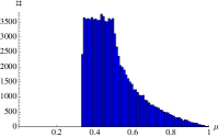
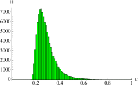
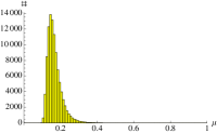
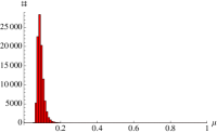
In Fig. 1 and in Fig. 2 we show the distributions of purity and nonG of the $10^{5}$ random quantum states for different dimensions of the Hilbert space. We notice that both these quantities distribute according to Gaussian-like distributions and, as said before, they concentrate around typical values increasing the dimension.

Figure 2: Histograms corresponding to the distributions of nonG of $10^{5}$ random quantum states for different dimensions of the Hilbert space. From left to right: $N=2$, $N=5$, $N=10$, $N=20$.

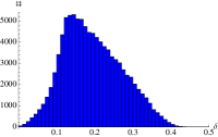
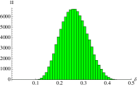
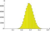
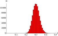
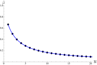
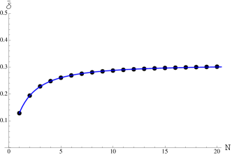
We also analyzed the behaviour of the average values, in particular we have looked for fitting functions $\overline{\mu}_{f}=\overline{\mu}_{f}(N)$ and $\overline{\delta}_{f}=\overline{\delta}_{f}(N)$ able to describe the behaviour of both $\overline{\mu}_{\hbox{\scriptsize N}}=\overline{\mu[\varrho]}_{\hbox{\scriptsize N}}$ and $\overline{\delta}_{\hbox{\scriptsize N}}=\overline{\delta[\varrho]}_{\hbox{\scriptsize N}}$ as a function of the maximum number of photons $N$, i.e. varying the dimension of the truncated Hilbert space $d=N+1$. The following fitting functions have been obtained

$$\overline{\mu}_{f}(N)=\frac{2}{N+2}\qquad\overline{\delta}_{f}(N)=-\frac{1}{(N+2)^{c_{1}}}+c_{2}$$ (3)

wit $c_{1}=1.560$ and $c_{2}=0.309$. These functions along with the corresponding numerical results are plotted in Fig. 3. If we study their behaviour when we consider Hilbert spaces with very high dimensions, i.e. with maximum number of photons $N\gg 1$, we observe that the typical purity vanishes as $2/N$ while the typical nonG approaches a finite value $\overline{\delta}_{\infty}\approx c_{2}$.

Figure 3: (Left) Black points: typical purity as a function of the maximum occupation number $N$. Blue line: fitting function $\overline{\mu}_{f}$ for the typical purity as a function of $N$. (Right) Black points: typical nonG as a function of the maximum occupation number $N$. Blue line: fitting function $\overline{\delta}_{f}$ for the typical nonG as a function of $N$.

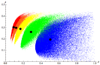
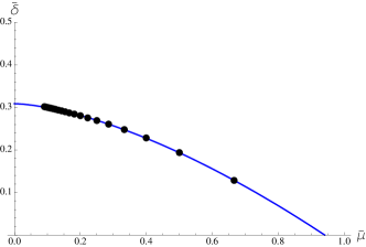
In order to better understand the relationship between the purity and the nonG of a truncated quantum state, we report the purity and the nonG of the generated states as points in the plane $(\mu,\delta)$. Results are shown in Fig. 4 where different colors denotes states generated in Hilbert subspaces with different dimensions. As it is apparent from the plot, the points concentrate, at fixed dimension, in well-defined regions of the plane, whose area decreases for increasing the dimension. Since, as mentioned above, upon increasing the dimension the typical nonG $\overline{\delta}_{\hbox{\scriptsize N}}$ increases and the typical purity $\overline{\mu}_{\hbox{\scriptsize N}}$ decreases, we have that higher typical nonG corresponds to lower typical purities. On the other hand, if we rather focus to points fixed dimension, we have that large values of nonG correspond to large values of purity, this effect being more pronounced for higher values of $N$.

   

Figure 4: Left: Purity and nonG of random states as points in the plane $(\mu,\delta)$. Different colors correspond to different dimension of the Hilbert space. The black points correspond to the average (typical) purity and nonG at each dimension. blue: $N=2$. green: $N=5$. yellow: $N=10$. orange $N=15$. red: $N=20$. Right: Typical purity and nonG in the plane $(\mu,\delta)$ varying the dimension $N=2,\dots,20$. The blue line correspond to the approximate formula reported in the text.

Using Eqs. (3) we may write the relation between the typical nonG and the typical purity as

$$\overline{\delta}_{f}(\overline{\mu})=c_{2}-\left(\frac{\overline{\mu}}{2}\right)^{c_{1}}\>.$$

Comparison with numerical findings is reported in the right panel of Fig. 4.

5 Conclusion

In conclusion, we have analyzed the properties of random quantum states generated in finite dimensional Hilbert spaces in terms of their nonG character and purity. We have found that both quantities distribute according to a Gaussian-like distribution with variance that decreases by increasing the dimension, i.e. they concentrate around typical values. We also found that the typical nonG and the typical purity are monotone functions of the dimension $d$. In particular, the average purity decreases to zero whereas the average nonG increases to an asymptotic value. Besides, we have found that, at fixed dimension, the points corresponding to the random states in the plane $(\mu,\delta)$ are confined in well-defined regions whose area decreases with the dimension. For increasing dimension higher nonG correspond to higher purities.

References

- [1] P. Walther et al., Phys. Rev. A 75, 012313 (2007).
- [2] B.M. Escher et al., Phys. Rev. 72, 045803 (2005)
- [3] L. A. de Souza et al., Phys. Lett. A 309, 5 (2003);
- [4] A.T. Avelar et al., Phys. Lett. A 318, 161 (2003).
- [5] K. Zyczkowski et al., Phys. Rev. A 58, 883 (1998).
- [6] K. Zyczkowski, Phys. Rev. A 60, 3496 (1999).
- [7] V. Cappellini et al., Phys. Rev. A 74, 062322 (2006).
- [8] J. Eisert et al., Int. J. Quant. Inf. 1, 479 (2003); A. Ferraro et al., Gaussian States in Quantum Information, (Bibliopolis, Napoli, 2005); F. Dell’Anno et al., Phys. Rep. 428, 53 (2006).
- [9] T. Opatrny et al., Phys.Rev. A 61, 032302 (2000).
- [10] P. T. Cochrane et al., Phys Rev. A 65, 062306 (2002).
- [11] S. Olivares et al., Phys. Rev. A 67, 032314 (2003).
- [12] N. J. Cerf et al., Phys. Rev. Lett. 95, 070501 (2005).
- [13] S. Olivares and M. G. A. Paris, J. Opt. B 7, S392 (2005).
- [14] T. Tyc at al., New. J. Phys. 10, (2008).
- [15] J. Wenger et al, Phys. Rev. Lett. 92, 153601 (2004).
- [16] M. G. Genoni et al., Phys. Rev. A 76, 042327 (2007).
- [17] K. Zyczkowski and M. Kus, J. Phys. A: Math. Gen. 27, 4235-4245 (1994).
- [18] K. E. Cahill and R. J. Glauber, Phys. Rev. 177, 1882–1902 (1969).
- [19] P. Marian et al., Phys. Rev. A 47, 4474 (1993); 4487 (1993).