Avalanche Statistics of Driven Granular Slides in a Miniature Mound

Abstract

We examine avalanche statistics of rain- and vibration-driven granular slides in miniature sand mounds. A crossover from power-law to non power-law avalanche-size statistics is demonstrated as a generic driving rate $\nu$ is increased. For slowly-driven mounds, the tail of the avalanche-size distribution is a power-law with exponent $-1.97\pm 0.31$, reasonably close to the value previously reported for landslide volumes. The interevent occurrence times are also analyzed for slowly-driven mounds; its distribution exhibits a power-law with exponent $-2.670\pm 0.001$.

JUANICO et al. AVALANCHE STATISTICS OF DRIVEN GRANULAR SLIDES… cmonterola@nip.upd.edu.ph,cmonterola@gmail.com

Gindraft=false

Introduction.—Landslides are the movement of a mass of rock, debris, or earth down a slope triggered by a variety of natural factors, ranging from rainfall to volcanic activity. On 17 February 2006, a series of mudslides caused widespread damage and loss of life in Southern Leyte, Philippines. The deadly landslides followed a ten-day period of persistent downpour and a minor ($M2.6$) earthquake (Catane et al., 2007).

One practical approach in analyzing the underlying physical processes that generate landslide statistics is numerical modeling. One class of models, based on self-organized criticality (SOC) (Hergarten and Neugebauer, 1998; Piegari et al., 2006), hint at some possible mechanisms yielding the observed statistics. SOC is a theory underlying the spontaneous emergence of critical-like behavior (i.e., power laws and critical exponents) in systems for which the timescales between buildup and release of stress are separated, and for which the stress-transfer mechanism is generally nonconservative (Juanico et al., 2007a; Juanico et al., 2007b; Juanico and Monterola, 2007). SOC concepts have aroused great interest in the study of granular matter (Jaeger et al., 1989), a well-known example of which is the ricepile experiment (Frette et al., 1996).

The present work examines avalanche statistics of rain- and vibration-driven granular slides in miniature sand mounds. A previous study (Katz and Aharonov, 2006) explored slope-failure types due to horizontal and vertical vibrations in a miniature sandbox. It was shown that vertical shaking leads to a power-law distribution of slide-block surface area, although the experiment did not demonstrate a ‘rollover’ observed in substantially complete, empirical landslide inventories (Guzzetti et al., 2002; Malamud et al., 2004a, b). In the present study, we incorporate rainfall as a triggering mechanism and show that its presence allows our model to capture the rollover. Likewise, we demonstrate experimentally the existence of a crossover from power-law to non power-law statistics as theoretically predicted by Piegari et al. (2006).

It appears from the data reported by Malamud et al. (2004a) that any type of trigger (earthquake, rainfall, or snowmelt) yields roughly the same trend in the landslide-size distribution. Combining any two trigger types should reasonably yield the same trend in the distribution, and this is precisely one of the aspects tested in this study. In addition, the computational model proposed here assumes a generic triggering mechanism. Thus, rainfall and vibrations have been introduced to act as concurrent landslide triggers.

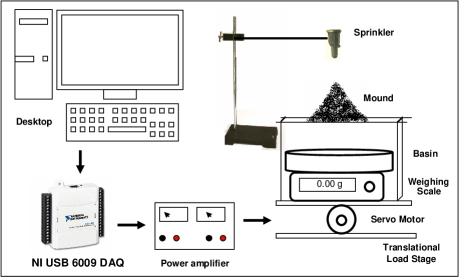
Experimental Method.—The experimental setup (Figure 1) consists of a sand mound (total mass, $1500$ g) disturbed concurrently by rainfall and vibration. River sand with irregularly-shaped grains (mean grain mass, $8.8\times 10^{-4}$ g; mean grain volume, $5.8\times 10^{-4}\,\,\mathrm{cm}^{3}$) was used. Initially, the mound is dry and is a near-perfect cone in shape with a base diameter of $23$ cm and height of $8$ cm (slope angle $\approx 35^{\circ}$ with respect to horizontal). Water ($200$ ml) is dispensed quite uniformly over the surface and allowed time to seep into the mound. The wet mound thus consists of $12$% water by weight at the start of the observations.

Rainfall is simulated using a makeshift sprinkler (water capacity, $75$ ml) placed directly above the mound apex. Water pours out through a circular orifice of diameters: $4.5$, $10.0$, and $47.0$ ($\pm 0.5$) mm. Pour rate is the mass of water flowing out per unit time, and the orifice diameter controls its value. Pour rate is constant at the following values: $3.21$ g $\mathrm{s}^{-1}$; $6.60$ g $\mathrm{s}^{-1}$; and $21.09$ g $\mathrm{s}^{-1}$ over a time interval of $20$, $10$, and $3$ s, respectively. These time intervals are commensurate with the length of time the 75-ml water in the sprinkler is depleted.

Horizontal vibrations are applied using a tabletop earthquake simulator. Horizontal shaking at low to moderate accelerations generates grain flows of the topmost layer of the slope resulting in rapid failure-plane development (Katz and Aharonov, 2006). As shown in Figure 1, a translational-load platform, powered by a servo motor driven by a USB $6009$ DAQ driver (National Instruments™), imparts the horizontal vibrations having a sawtooth wave profile. The wave profile is fed into the DAQ driver via LabVIEW™computer interface. The wave is characterized by a maximum amplitude of $1.5$ cm (with respect to center) and by frequencies of: $1.8$ Hz, $10$ Hz, and $89$ Hz. Due to the 3D shape of the mound, slope-parallel and slope-normal accelerations are both present during shaking.

Computational Model.—The underlying physics of the avalanche statistics of driven granular slides is investigated by performing numerical experiments of a landslide model proposed by Piegari et al. (2006), defined as follows. A mountain ‘slope’ is represented as a 2D inclined plane partitioned into a grid ($500\,\,\mathrm{cells}\,\times\,500\,\,\mathrm{cells}$). Each cell $k$ is described by a stress parameter $\theta_{k}$ initialized randomly between $0$ and $1$ from an arbitrarily chosen rectangular distribution (although the distribution used for initial randomization does not affect the long-term behavior of the model (Piegari et al., 2006)). The randomization captures the expected heterogeneity of stress values in actual mountain slopes. Stress in the slope builds up over time by means of a localized (i.e., cell scale) driving: $\theta_{k}\left(t+\Delta t\right)=\theta_{k}(t)+\nu\Delta t$, where $\nu$ is the generic driving rate. For simplicity, it is assumed that $\nu$ has the same value for all cells. When a cell $k$ has $\theta_{k}>1$, it relaxes by transferring stress to its four nearest neighbors $nn=\left\{up,down,right,left\right\}$ at different proportions $g_{nn}$. By virtue of gravity, stress transfer is biased downwards, such that: $g_{down}>g_{up}$, subject to the constraint $g_{down}+g_{up}=0.5$; and $g_{left}=g_{right}=0.25$. In this study, it is assumed that transfer is conservative, so that $\sum_{nn}g_{nn}=1$. Stress-transfer proceeds until the entire grid relaxes so that for all $k$, $\theta_{k}<1$. All consecutive stress-transfers comprise a landslide at time $t$, and the total number of collapsing cells at time $t$ is the landslide area $A(t)$. For correspondence with experiments, although we recognize its limitations, we assume a landslide mass-area relation: $M\sim A^{3/2}$, which can be derived by means of dimensional analysis (i.e., assuming that $M$ is proportional to volume $V$, and then considering that $V\sim A^{3/2}$ (Hovius et al., 1997)).

The novelty of our computational modeling approach is in considering the gradual flattening of the slope after several landslides have occurred (as seen in our experiments). An update rule is introduced to decrease $g_{down}$, as follows: $g_{down}(t+\Delta t)=g_{down}(t)-10^{-5}A(t)$, where $A(t)$ is the area of landslide at time $t$. The value of $g_{up}$ is updated accordingly via the constraint $g_{down}+g_{up}=0.5$. This modification incorporates the dynamics of slope evolution which was not realized by Piegari et al. (2006). The generic driving rate $\nu$ defined in the model corresponds to the experimental parameters, as shown in Table 1.

Table 1: Generic driving rate $\nu$ in terms of experimental parameters

Description	Driving rate (no units) $\nu$	Pour rate (g $\mathrm{s}^{-1}$)	Vibration frequency (Hz)
Slow	$7.50\times 10^{-5}$	3.21	1.8
Moderate	$1.25\times 10^{-4}$	6.60	1.8, 10, 89
Fast	$7.50\times 10^{-4}$	21.09	1.8, 10, 89

Results and Discussion.—Avalanche size is interpreted as the total mass $M$ of wet sand falling from the mound onto the basin within a $20$-ms period (temporal resolution of our data-capturing device). $M$ is measured by a weighing scale (resolution, $0.1$ g) beneath the basin, as illustrated in Figure 1. $M$ is sometimes contributed to by several distinct ‘sub-avalanches.’ The tradeoff in this interpretation is that although it resolves mostly individual avalanches, those that last $>20$ ms may be recorded as partial sub-avalanches, and if there are more than one avalanche within any $20$ -ms interval, these will be recorded as one value.

The total observation period is determined by the pour rate and is based on how long before the entire mound washes out. A total of $20$, $10$, and $3$ trials were made for slow, moderate, and fast pour rates, respectively. The fact that sand tends to stick together when wet (i.e., negative pore pressure) (Katz and Aharonov, 2006) justifies our assumption that by measuring the mass $M$ of falling wet sand, the avalanche volume is effectively measured (i.e., $M\propto V$). In (Malamud et al., 2004a, b), the distribution of landslide volumes has been deduced from scaling arguments due to the difficulty in obtaining direct information about landslide volume from field data (Malamud et al., 2004a). In our experiment, landslide volume distribution is determined by using mass as a proxy for volume.

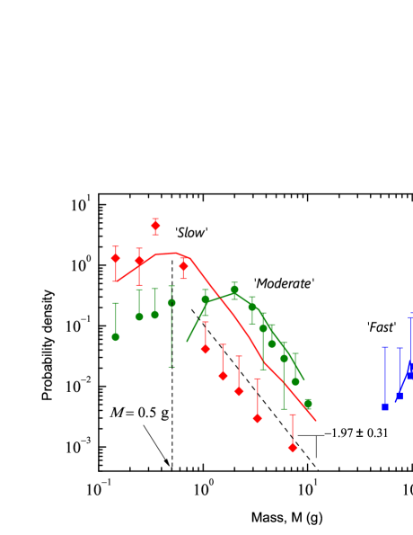
Figure 2 illustrates probability densities (pdf) of avalanche sizes resulting from slow ($\blacklozenge$), moderate ($\bullet$), and fast ($\blacksquare$) driving (as defined in Table 1). Also shown are corresponding pdfs from numerical simulations of the computational model. The pdfs for all cases exhibit peaks that shift towards the right as the driving rate is increased. In particular, The tail of the pdf for a slowly-driven mound ($\blacklozenge$, Fig. 2) is a power-law with exponent $-1.97$($\pm 0.31$; standard error of least-squares fit, $df=4$, reduced $\chi^{2}=1.14\times 10^{-5}$), determined by curve-fitting the linear portion (in double log scale) for which $1.0\,\,\mathrm{g}<M<8.0\,\,\mathrm{g}$. The exponent value is not significantly different (two-tailed $t$-test: $t=1.13$, $df=4$, $p=0.32$) from the value $-1.93$ reported for probability densities of landslide volumes (Malamud et al., 2004a).

A crossover from power-law to non power-law statistics is also evident in our data. This crossover has been previously recognized by Piegari et al. (2006) as an effect of increasing the generic driving rate $\nu$. We attribute the crossover to timescale separation. Based on the model, the timescale separation is the ratio between the timescale $\nu^{-1}$ of stress changes on any site due to driving and the timescale of the longest avalanche which is set at $\Delta t=1$. Hence, the timescale separation is $\left(\nu\Delta t\right)^{-1}\sim\nu^{-1}$. For slow driving (small $\nu$), SOC theory expects the appearance of power laws. On the other hand, for fast driving, a different trend is expected. We found this fit to resemble a normal distribution, and is centered at a large $M$ ($\blacksquare$, Fig. 2). An implication of the crossover is that under high-rate driving (especially by frequent rainfall), the landslide behavior of mountain slopes appears to produce relatively large avalanches on average. It is thus not surprising that highly-devastating rain-induced landslides occur more often in areas frequently struck by storms. However, a more comprehensive description of $\nu$ should incorporate ground-failure factors such as soil composition. Such factors have been neglected in this study for simplicity.

The rollover observed in our data supports the claim that the rollover seen in substantially complete landslide-inventory datasets is not a mere artifact of limited mapping resolution  (Guzzetti et al., 2002; Malamud et al., 2004a, b). As $\nu\rightarrow 0$ , the rollover is expected to disappear thus leaving the power-law tail of the distribution. This agrees with predictions from the Olami-Feder-Christensen model (Olami et al., 1992), which is the limiting case of our model for $\nu\rightarrow 0$. To the extent that our experiment and numerical results agree, we thus attribute the rollover to the finiteness, albeit small, value of the driving rate $\nu$ assumed to characterize real physical systems. From this argument it can thus be reasonably deduced that the rollover increases in prominence, such that the peak shifts towards larger avalanche sizes, as $\nu$ increases. We found that at $\nu\sim 7.5\times 10^{-4}$, the avalanche size distribution more closely resembles a normal (or Gaussian) distribution that is centered at a large size value.

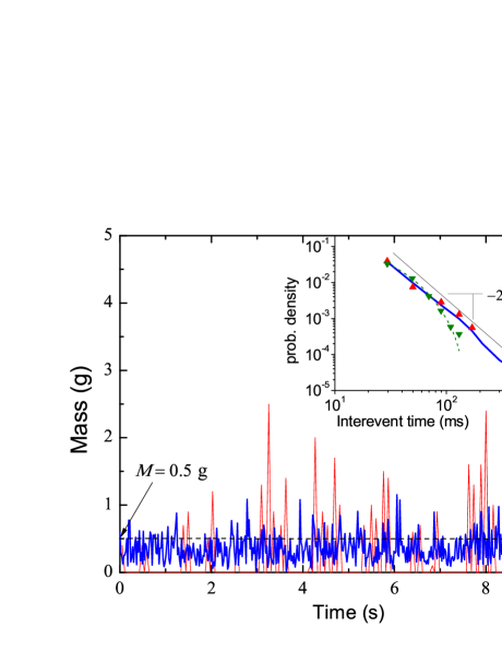
A relevant aspect for hazard prediction is the interevent occurrence time (IOT) statistics. The IOT is the interval between the peaks of events whose sizes are above a given threshold ($M=0.5$ g), which corresponds roughly to the peak of the pdf ($\blacklozenge$, Figure 2). We thus gathered time series of avalanche size $M(t)$ in slowly-driven mounds over a period of 20 s. Figure 3 illustrates a representative sample for the first 10 s of this time series for both experiment and computational data. A thresholding procedure is applied to discard events whose sizes are below the threshold. The region $M<0.5$ g corresponds to the rollover portion of the pdf ($\blacklozenge$, Figure 2) for slowly-driven mounds. The vertical demarcation line in Figure 2 corresponds to the horizontal demarcation line in Figure 3. The probability density for interevent occurrence time derived from experiment and model are shown on the inset graph of Figure 3 ($\blacktriangle$; blue, solid curve), and both exhibit a power-law trend with exponent $-2.670$($\pm 0.001$; standard error of least-squares fit, $df=6$, reduced $\chi^{2}=2.09\times 10^{-8}$).

A power-law IOT distribution implies that most correlated events (i.e., those with sizes above the threshold) tend to occur close together in time, which seems to agree with recent findings (Rossi et al., 2008). The power-law trend further implies that correlated events may be separated a long time from each other—a landslide today may be linked with an earlier landslide a long time ago. This may be tied to the fact that landslides tend to occur where they have occurred before. The long temporal correlation suggested by the power-law could possibly be attributed to rainfall seasonal trends (Rossi et al., 2008).

To illustrate that a power-law emerges from temporal correlations in the time series data, a shuffling procedure has been implemented wherein the order of the time series is rearranged randomly (Yang et al., 2004). Random shuffling effectively eliminates any trace of correlations present in the original time series data. The thresholding procedure is then applied on the shuffled data to extract the IOT distribution. After shuffling, the IOT distribution becomes exponential, as shown in Figure 3 ($\blacktriangledown$, Inset). The change from power-law to exponential due to shuffling has been expected for systems governed by SOC dynamics (Woodward et al., 2004). Therefore, we conclude that the power-law is a direct indication of temporal correlations in the time series data.

Conclusion.—The general agreement of our results with empirical data suggests that miniature experimental models may help in understanding several underlying facets of complex landslide processes. While several geophysical factors such as sand porosity, rock type, pore-water pressure, and humidity have been neglected, the landslide model presented here delivers basic insights that would guide more detailed explorations later on.

Figure 1: Diagram of experimental setup. Sand mound consists of river sand. Rainfall is simulated by a sprinkler right above the mound apex. An earthquake is simulated by a translational load stage imparting horizontal vibrations to the platform where the mound is placed. Rainfall and vibration are parametrized by pour rate and vibration frequency, respectively. Different parameter combinations are listed on Table 1. Avalanche size is the mass $M$ of wet sand falling onto the basin within $20$-ms intervals. $M$ is measured by a weighing scale at the bottom of the basin, and is connected to the PC that records measurements in time.

Figure 2: (Color online). Probability densities (pdf) of avalanche sizes. Pdfs for slow ($\blacklozenge$), moderate ($\bullet$), and fast ($\blacksquare$) driving; where the error bars are $\pm 2\sqrt{n}/\delta$ (equivalent to $\pm 2\sigma$, 95% confidence; $n=$ number of values in a bin; and $\delta$ is the bin width). Corresponding pdfs of avalanche size from numerical simulations (curves) are overlaid, after converting area into mass using the scaling relation: $M=(1.0\times 10^{-5}\mathrm{g}\cdot\mathrm{cell}^{-3/2})A^{3/2}$. Linear regime ($1.0<M<8.0$ g) of the pdf for a slowly-driven mound fits a power-law with exponent $-1.97\pm 0.31$. For moderately-driven mounds, the rollover region of the pdf becomes more prominent as the peak shifts to the right. For highly-driven mounds, the pdf resembles a normal distribution centered at a large $M$.

Figure 3: (Color online). Interevent occurrence times (IOT). Time series of avalanche sizes from experiment (red, solid curve) and model (blue, thick curve). Consecutive data points are separated by $20$ ms. Iteration steps (iter) in the model have been rescaled to time by multiplying by the scaling factor: $0.05\,\mathrm{s}\cdot\mathrm{iter}^{-1}$. Avalanche sizes less than $0.5$ g are discarded. IOT is the interval between consecutive peaks above the threshold. Inset: IOT distributions for experiment ($\blacktriangle$) and model (blue solid curve) both exhibit a power-law with exponent $-2.670\pm 0.001$. Randomly shuffling the order of the time series effectively results in an exponential IOT distribution ($\blacktriangledown$; curve fit: green, dashed curve).