Critical properties of edge-cubic spin model on square lattice

Abstract

The edge-cubic spin model on square lattice is studied via Monte Carlo simulation with cluster algorithm. By cooling the system, we found two successive symmetry breakings, i.e., the breakdown of $O_{h}$ into the group of $C_{3h}$ which then freezes into ground state configuration. To characterize the existing phase transitions, we consider the magnetization and the population number as order parameters. We observe that the magnetization is good at probing the high temperature transition but fails in the analysis of the low temperature transition. In contrast the population number performs well in probing the low- and the high-$T$ transitions. We plot the temperature dependence of the moment and correlation ratios of the order parameters and obtain the high- and low-$T$ transitions at $T_{h}=0.602(1)$ and $T_{l}=0.5422(2)$ respectively, with the corresponding exponents of correlation length $\nu_{h}=1.50(1)$ and $\nu_{l}=0.833(1)$. By using correlation ratio and size dependence of correlation function we estimate the decay exponent for the high-$T$ transition as $\eta_{h}=0.260(1)$. For the low-$T$ transition, $\eta_{l}=0.267(1)$ is extracted from the finite size scaling of susceptibility. The universality class of the low-$T$ critical point is the same as the $3$-state Potts model.

I Introduction

The presence of symmetry breaking in many areas of physics such as particle, atomic and condensed matter physics is indicative of the importance of the phenomenon zinn . In general, the breakdown of symmetry is an onset of a phase transition which separates phases with different degrees of symmetry landau . A system is in high degree of symmetry at high temperature because it is able to explore all its configurational spaces. The decrease in temperature will reduce thermal fluctuation and lead the system to stay in some favorable states. This type of transition with no co-existence phases, therefore no latent heat, is commonly called a continuous phase transition.

A system with initially large number of symmetry elements is more likely to experience sequential phase transitions. In fact, various magnetic systems exhibit such behavior. The clock spin model in two dimensions, for example, whose group symmetry $C_{n}$ experiences double Kosterlitz-Thouless transitions for $n>4$ jose . In the presence of frustration which induces chiral symmetry $Z_{2}$, another phase transition occurs tasrief04 .

In this paper, we study the edge-cubic spin model on two dimensions. The model is one of the discrete counterparts of the continuous-spin, the Heisenberg model, of symmetry group ($O_{3}$). In two dimension anisotropy is important as systems with discrete symmetry can have a true long range order at finite temperature. The octahedral symmetry group $O_{h}$ of the model, with 48 symmetry elements, consists of some subgroups associated with familiar discrete models, such as the inversion $Z_{2}$ of Ising model and the $C_{3h}$ of the chiral 3-state Potts model. Any finite ordered phase of the system is expected to be in one of its subgroup symmetries.

While cubic symmetry in magnetic systems is an old subject and appears whenever systems are on real cubic lattice aharony ; kim , cubic spin models have not been studied as much as other discrete models such as Ising, Potts and clock models. Previous works on cubic symmetries were mostly carried out in the theoretical field approach through the consideration of the $\phi^{4}$ Hamiltonian in which $n$-component anisotropy fields break the continuous $O(N)$ symmetry sznajd ; calabrese02 . It is well established that for three-dimensional case, the cubic fixed point is stable if $n>n_{c}$, where $n_{c}<3$ according to more recent calculations calabrese02 ; carmona . The situation is different in two-dimensional case because the existence of cubic fixed point is still unclear. Recent study by Calabrese et al. could not unravel the speculation that the Ising and the cubic fixed points maybe coincide calabrese04 .

In trying to resolve the speculation of the existence of cubic fixed point in two dimensions, it is of importance to directly probe the spin models with cubic symmetry. With simple normalized-vector spin on cube, we can have three models i.e, the face-cubic (6 states), the corner-cubic (8 states) and the edge-cubic spin (12 states). Very recently, Yasuda et al. yasuda considered a ferromagnetic face-cubic spin model and then found that the model undergoes a single phase transition; they discussed the universality class of this model in comparison with 4-state Potts model. The corner-cubic spin model is considered as a trivial model of decoupled three independent Ising models. Studying the corner-cubic model can not be expected to address the existence of cubic fixed point. However, by weighting the spin orientation, the corner-cubic spin model can transform into a general Ashkin-Teller model ashkin ; to this respect the model is no longer trivial.

Probing the edge-cubic spin model deserves for its own right. Firstly, it is interesting to know the symmetry breaking of the $O_{h}$ in that model, and also to address the existence of cubic universality class. Since the degree of $O_{h}$ is high, the edge-cubic model may experience sequential phase transitions.

The remaining part of the paper is organized as follows: Section II describes the model and the method. The result is discussed in Section III. Section IV is devoted to the concluding remarks.

II Model and Simulation Method

The edge-cubic spin model is one of the discrete counterparts of the Heisenberg model. Spins can point to any of the 12 middle points of the edges of a cube. An edge of the cube is 2 unit long, and its center of mass $O(0,0,0)$ is set as the origin of the normalized-vector spin. Here we study the ferromagnetic case on square lattice with periodic boundary condition. The Hamiltonian of the model is expressed as

$$H=-J\sum_{\langle ij\rangle}\vec{s}_{i}\cdot\vec{s}_{j}$$ (1)

where $\vec{s}_{i}$ is a spin on site $i$-th, $J>0$. Summation is performed over all the nearest-neighbor pairs of spins. In the ground state configuration, i.e., when all spins having a common orientation, the energy will be $-2JN$ with $N$ is the number of spins.

Figure 1: The temperature dependence of the specific heat for various system sizes. As shown, there exist a clear peak and a hump respectively at high and at low temperatures. The peak and the hump signify that system possesses sequential phase transitions. The error bar, in average, is in the order of symbol size, except data for $L=256$ at $T>0.65$, where error is larger than the symbol size.

We use the canonical Monte Carlo (MC) method with single cluster spin updates due to Wolff wolff and adopt Wolff’s idea of embedded scheme in constructing a cluster for the edge-cubic spins. This is done by projecting the spins into a randomly generated plane so that the spins are divided into two groups (Ising-like spins). The embedded scheme is essential in carrying out cluster algorithm for such spins as cubic and planar spins.

After the projection, the usual steps of the cluster algorithm are performed kasteleyn , i.e., by connecting bonds from the randomly chosen spin to its nearest neighbors of similar group, with suitable probability. This procedure is repeated for neighbors of sites connected to chosen spin until no more spins to include. One Monte Carlo step (MCS) is defined as visiting once the whole spins randomly and perform cluster spin update in each visit. Note that a spin may be updated many times, in average, during one step, in particular near the critical point.

Measurement is performed after enough equilibration MCS’s ($10^{4}$ MCS’s). Each data point is obtained from the average over several parallel runs, each run is of $4\times 10^{4}$ MCS’s. To evaluate the statistical error each run is treated as a single measurement. For the accuracy in the estimate of critical exponents and temperatures, data are collected upto more than 100 measurements for each system size.

III Results and Discussion

III.1 Specific heat and magnetization

The first step in search for any possible phase transition is to measure the specific heat of the system defined as follows

$$C_{v}(T)=\frac{1}{Nk_{B}T^{2}}(\langle E^{2}\rangle-\langle E\rangle^{2})$$ (2)

where $E$ is the energy in unit of $J$ while $\langle\cdots\rangle$ represents the ensemble average of the corresponding quantity. All temperatures are expressed in unit of $J/k_{B}$ where $k_{B}$ is the Boltzmann constant.

Figure 2: Temperature dependence of (a) moment ratio and (b) correlation ratio for several system sizes. The crossing points indicates a phase transition between the disordered and the intermediate phase. A cusp in the moment ratio and valley-like in the correlation ratio suggest another phase transition. Error bar is in the order smaller than the symbol size.

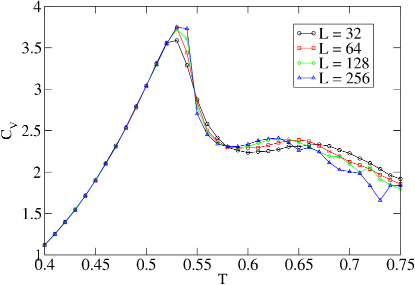
As shown by the specific heat plot in Fig. 1, there exist a peak at lower temperature and a hump at higher temperature. Although the peak and the hump are more directly related to energy fluctuation, they may signify the existence of sequential phase transitions. In what follows, more quantitative analysis is performed through the evaluation of the order parameters.

The critical properties of the system are quantified by the critical temperatures and exponents extracted from the finite size scaling (FSS) of the order parameters, in particular from their moment and correlation ratios. As the probed system is ferromagnetic we consider magnetization $M=|\sum\vec{s}_{i}|$ as the order parameter. By defining $M^{k}$ as the $k$-th order moment of magnetization and $g(R)=\sum\vec{s}(r)\cdot\vec{s}(r+R)$ as correlation function, the moment and correlation ratios are respectively written as follows

$$U_{L} = \frac{\langle M^{4}\rangle}{\langle M^{2}\rangle^{2}}$$ (3)

$$Q_{L} = \frac{\langle g(L/2)\rangle}{\langle g(L/4)\rangle}$$ (4)

Precisely, the distance $R$ for the correlation function $g(R)$ is a vector quantity, here we take the simple form and choose convenient distances $L/2$ and $L/4$, both in $x$- and $y$-directions.

Figure 3: The FSS plot of (a) moment ratio, (b) correlation ratio. The estimates of critical temperature and the exponent of correlation length $\nu$ are obtained.

Figure 4: Double logarithmic plot of $g(L/2)$ vs $L$ for several values of correlation ratio $Q_{L}$’s. The best estimate of $\eta=0.260(1)$ is the slope of the best-fitted line of $Q_{L}=0.91$ associated with critical temperature.

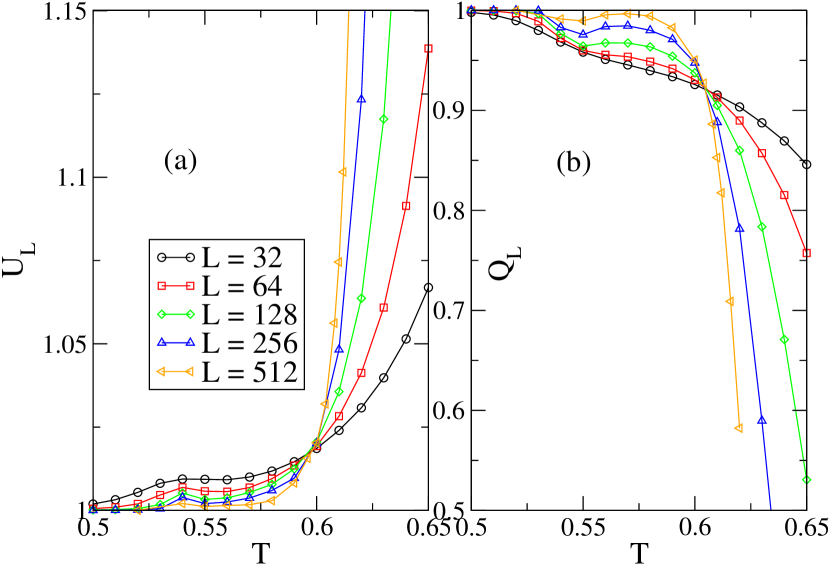
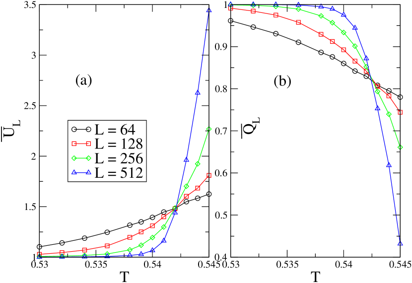
More accurate estimate of parameters of phase transition is obtained from the temperature dependence of $U_{L}$ and $Q_{L}$. At very low temperature where system is approaching the ground state, both moment and correlation ratio are trivial. Due to the absence of fluctuation, the distribution of $M$ is a delta-like function, giving moment ratio equals to unity. Correlation ratio also goes to unity as correlation function for small and large distance is the same due to highly correlated states. In excited states, the moment and the correlation ratios are not trivial, they depend on temperature. The plot of moment ratio for various system sizes, shown in Fig. 2(a), exhibits a clear crossing point which indicates a phase transition. At low temperature side, there exists a cusp which may corresponds to another phase transition. A possibility that system has additional phase transition at low temperature, apart from an obvious one at high temperature, is also signified by the plot of correlation ratio shown in Fig. 2(b).

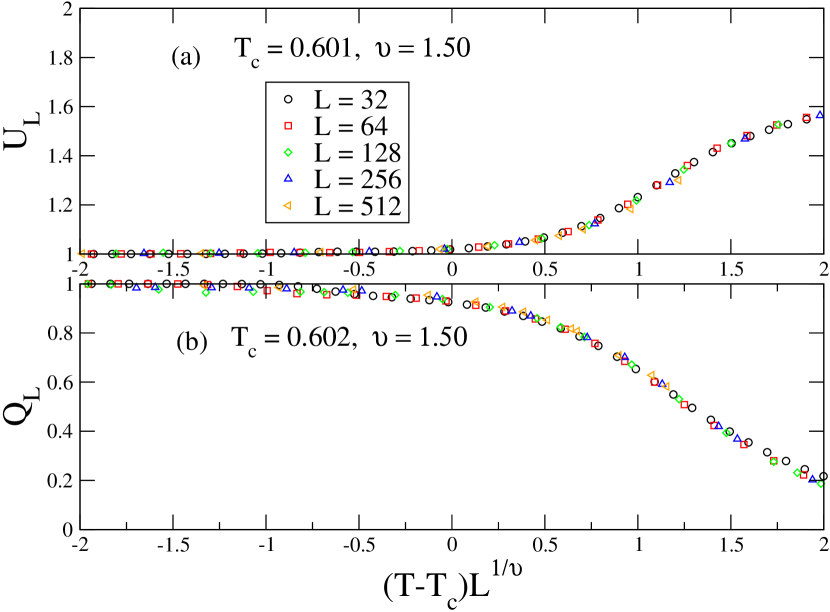
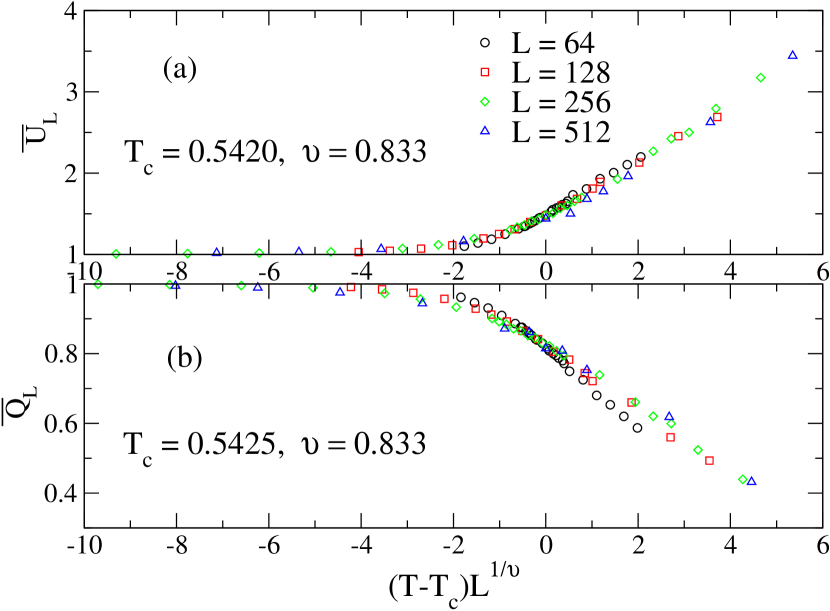
We show the FSS plot of moment and correlation ratios in Fig. 3; we estimate critical temperature and exponents from both ratios which give consistent results, with only difference smaller than estimated statistical error. The estimate of $T_{c}$ obtained from moment ratio is $T_{c}=0.601(1)$, slightly smaller than $T_{c}=0.602(1)$ from the correlation ratio. The number in bracket is the uncertainty in the last digit. In general, moment ratio has larger correction to scaling than the correlation ratio tomita02a , which happens to be the case here. However, if the variables of the two correlation functions are not local quantity, in the sense they depend on another quantity, then the correlation ratio may have larger correction to scaling. Our estimate of $T_{c}$ is based on result obtained from the correlation ratio. The estimates of the decay exponent of the correlation length both give the same results, i.e., $\nu_{h}=1.50(1)$. The subscript is used for the reminder that we are dealing with the high-$T$ transition.

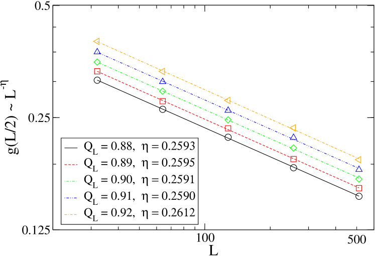
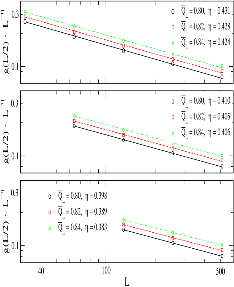
In addition to the exponent $\nu$, it is possible to extract the decay exponent $\eta$ of the correlation function from the correlation ratio. This is done by firstly looking at the constant value of correlation ratio $Q_{L}$ for different sizes and then find the corresponding correlation function $g(L/2)$. The correlation function is in power-law dependence on the system size, $g(L/2)\sim L^{-\eta}$ tomita02a . Therefore, if we plot $g(L/2)$ versus $L$ for various $Q_{L}$’s in logarithmic scale, as in Fig. 4, the value of $\eta$ will correspond to the gradient of the best-fitted line for each constant of correlation ratio. There are several lines plotted in Fig. 4. Since the critical temperature is associated with the value of $Q_{L}\sim 0.91$ (Fig. 2(b)), we assign $\eta=0.260(1)$ as the best estimate.

Figure 5: The cube and 1/8 cube (green). Three outer sides of the small cube viewable from corner (111) are the surfaces penetrated by series of magnetization vectors.

Although there is an indication of low temperature transition, at this stage we do not estimate its critical quantities due to the absence of a crossing point. We need to formulate a more suitable order parameter able to distinguish the intermediate and the low temperature ordered phase. In the next section, we present the snapshot series of total magnetization and discuss the order parameter of characterizing low temperature transition.

III.2 Snapshot of spin configuration and population number order parameter

Figure 6: Plot of the series of snapshots of total magnetization. The orientation is viewed from the corner point (111) of the cube. Each symbol represents the total magnetization of a snapshot spin configuration.

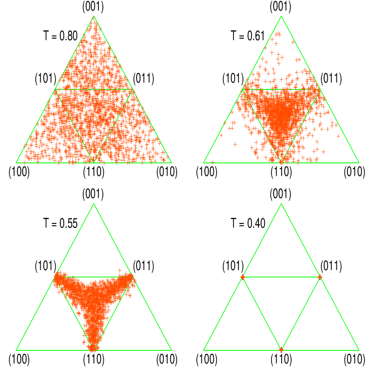
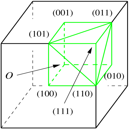
The total vector magnetization is computed for every snapshot spin configuration. A snapshot magnetization is represented by a dot that is the intersection of the line parallel to the magnetization and the cube surface. Thus we obtain dots as many as the number of MCS’s, and we view this dots from the (111) direction as shown in Fig. 5.

Figure 7: Plot of temperature dependence of population number, $M_{i}$ i.e., the thermal average of number of spins pointing to $i$-th direction. At each MCS, 12 possible directions are sorted and we assign the most populated as $M_{1}$, the second largest as $M_{2}$, and so on. Here the linear size of the lattice is $L=128$.

For simplicity, we make suitable mirror projection of the total magnetization so that its orientation is in the region of the three outer sides of the 1/8 cube. We further project the surface of the 1/8 cube on to a triangle as shown in Fig. 6. The inner triangle is associated with the plane made by three edge-points ((101), (110) and (011)) in Fig. 5. Each pair of these points together with a middle point of sides viewable from the corner point (111) construct three other outer triangles.

The phase of the system is related to spin configuration. At high temperatures, due to large thermal fluctuation, each spin is relatively free to point to any direction, therefore no common orientation of the total magnetization. As a result, the snapshot point will occupy the whole area of four triangles. This is indicated by the Fig. 6 with $T=0.80$.

As we reduce the temperature, the thermal fluctuation starts being overcome by the magnetic interaction. The snapshot points start being around the middle area of the triangle (associated with $T=0.61$). At this state, three neighboring spin-orientations near a corner of the cube become more favorable. At temperature $T=0.55$ system is in intermediate phase where almost all snapshots are inside the area of the inner triangle. Three neighboring orientations around a particular corner of the cube are chosen; the octahedral symmetry $O_{h}$ is completely broken.

The symmetry group associated with the intermediate phase is the point group $C_{3h}$, realized for example by the 3-state Potts model. As the temperature is further reduced, this symmetry breaks down into a ground state with all spins pointing to the same direction, shown by the figure with $T=0.40$. Therefore, from the symmetry group point of view, it is natural to expect that the low temperature phase transition is in the same universality class as the 3-state Potts model.

Figure 8: Temperature dependence of (a) moment ratio and (b) correlation ratio for the occupation number order parameter defined in Eq. (5). Error bar is in the order of symbol size.

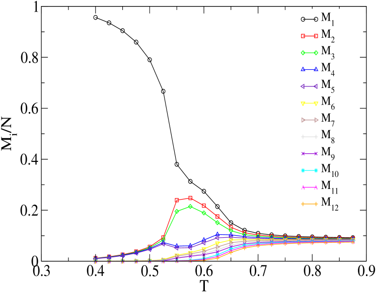
Based on the snapshot of magnetization, we define an order parameter related to population numbers. It is formulated from the fact that at each microscopic state, spins will be pointing to 12 possible orientations. The difference between maximum population among the 12 orientations and the second largest is assigned as the order parameter which is written as follows

$$\bar{M}=M_{1}-M_{2}$$ (5)

where $M_{1}$ and $M_{2}$ are the largest and the second largest population numbers, respectively.

At ground state the value of this order parameter will be just $N$ because all $N$ spins are in a common alignment. In contrast, at high temperature, the value of the order parameter is very small and vanishing in the thermodynamic limit, as the 12 possible orientations are occupied by approximately equal number of spins. Figure 7 shows the temperature dependence of the 12 population numbers $M_{i}$. One could choose another quantity as an order parameter, but Eq. 5 is simple and straightforward.

The breakdown of symmetries experienced by the system can also be detected from temperature dependence of $M_{i}$. At high temperature side ($T>0.8$), 12 lines are approximately parallel. There is a clear split of lines at temperature around $T=0.61$, where 3 lines go up whereas the others go down. This reminds us of Fig. 6 with $T=0.61$, where three neighboring spins around a cube corner start being favorable. At lower temperatures ($T<0.55$), the upper three lines separate into two groups, where one continuously goes up while the other two are vanishing. This exhibits the breakdown of $C_{3h}$.

Figure 9: Finite size scaling plot of (a) moment ratio and (b) of Fig. 8.

In this part, we make use the moment and the correlation ratio of the newly introduced order parameter for the analysis of the low temperature critical behavior, expressed as

$$\bar{U}_{L} = \frac{\langle\bar{M}^{4}\rangle}{\langle\bar{M}^{2}\rangle^{2}}$$ (6)

$$\bar{Q}_{L} = \frac{\langle\bar{g}(L/2)\rangle}{\langle\bar{g}(L/4)\rangle}$$ (7)

Here, the correlation function $\bar{g}(R)=\sum\bar{M}(R+r)\bar{M}(r)$, where $\bar{M}(R)$ is defined as follows

$$\bar{M}(R)=M_{1}(R)-M_{2}(R)$$ (8)

where $M_{k}(R)$ is 0 or 1. When the spin at $R$, $\vec{s}(R)$, is in the $k$-th populated direction $M_{k}(R)=1$, otherwise it is 0. This means the direction 1 (or 2) can be different for different Monte Carlo steps. With this definition, the correlation function relates points with functional variable of occupation number. The plot of these ratios for various system sizes, given in Fig. 8, has shown a clear crossing point separating between the intermediate and the low temperature order phases. The FSS plot of the moment and correlation ratios, shown in Fig. 9, gives the estimates of $T_{c}$ and the exponent $\nu$. While the quality of the plot is not as good as that of the susceptibility discussed below, we estimate $T_{c}=0.5422(2)$ and $\nu=0.833(1)$ based on moment ratio. This exponent is in a good agreement with the result of 3-state Potts model wu .

The decay exponent $\eta$ for the correlation function of $\bar{M}$ can also be extracted in the same way for $M$. After determining a fixed value of correlation ratio, we search for $\bar{g}(L/2)$ of each system size and plot against $L$ in logarithmic scale. The gradient of the best-fitted line associated with critical value of correlation ratio is the estimate of $\eta$. However, due to large correction to scaling of the correlation ratio, the estimates of $\eta$ is off from the 3-state Potts model. By excluding the small system sizes, as indicated in Fig. 10, the estimated value of $\eta$ systematically declines. We believe that the value of the 3-state Potts model is approached for larger system sizes.

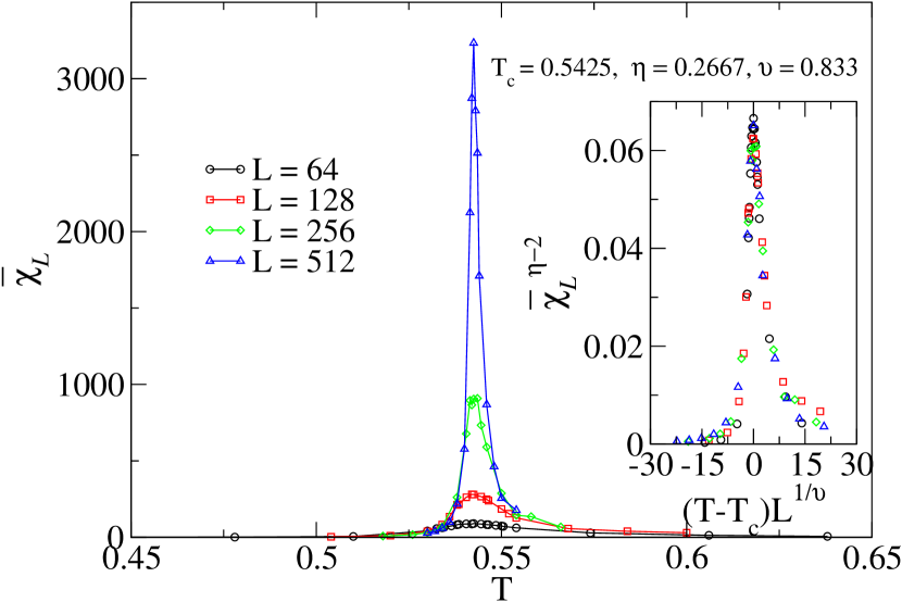
In order to obtain a better estimate of $\eta$, we perform another approach, namely by using the FSS of susceptibility $\chi_{L}$, which is written as follows

$$\bar{\chi}_{L}=L^{2-\eta}\tilde{\bar{\chi}}_{L}\left((T-T_{c})L^{1/\nu}\right),$$ (9)

where $\bar{\chi}_{L}=\left(\langle\bar{M}^{2}\rangle-\langle\bar{M}\rangle^{2}\right)/L^{2}$. The temperature dependence of $\bar{\chi}_{L}$ is given in Fig. 11 with the inset is its FSS plot. The exponent $\nu=0.833(1)$ and $\eta=0.267(1)$ belong to 3-state Potts model.

Figure 10: Double logarithmic plot of $\bar{g}(L/2)$ vs $L$. The gradient of the fitted line associated with $\bar{Q}_{L}=0.82$ is the estimate of $\eta$. By excluding the smaller system sizes, the value of estimated $\eta$ systematically increases, which indicates large correction to scaling.

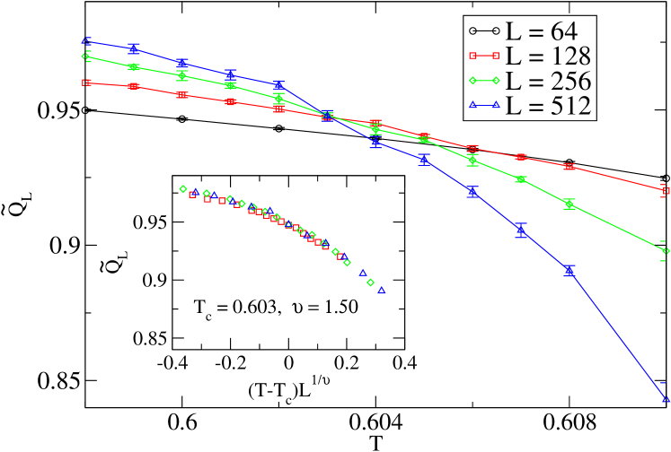
Next, we address the possibility of characterizing the high temperature transition by using the order parameter based on population number. Obviously, the order parameter introduced in Eq. (5) is only appropriate for low temperature, not for high temperature transition. This is due to the fact that at high and intermediate temperatures, $M_{1}$ and $M_{2}$ have approximately similar value, especially for larger system sizes. In the intermediate phase, the three neighboring spin-orientations are favorable; thus for probing high temperature transition, it is appropriate to subtract $M_{4}$, the fourth largest population number, instead of $M_{2}$, from $M_{1}$, and obtain $\tilde{M}=M_{1}-M_{4}$, analogous to Eq. (5). The temperature dependence of the correlation ratio and its FSS is shown in Fig. 12. The plot of temperature dependence for various system sizes gives a crossing critical point. The estimate of $T_{c}=0.603(2)$ and $\nu=1.50(1)$ is consistent with that obtained earlier.

Figure 11: Temperature dependence of susceptibility and its FSS (inset). The exponents $\eta$ and $\nu$ are very consistent with that of 3-state Potts model.

Figure 12: Correlation ratio of the order parameter $\bar{M}=M_{1}-M_{4}$ vs temperature. There is a clear crossing point for curves of larger system sizes, $L$ = 128, 256, and 512. The system size $L=$ 64 seems to have quite large correction to scaling. The inset is the FSS for the 3 large system sizes.

After obtaining the critical exponents, we can now discuss the universality classes of the phase transitions. Two symmetry breakings are obvious from the snapshot series of magnetization shown in Fig. 6 as well as from temperature dependence of $M_{i}$ in Fig. 7. At higher temperature, the native octahedral symmetry $O_{h}$ breaks into an intermediate phase $C_{3h}$ symmetry which then freezes into a ground state of low temperatures. The high temperature phase transition with exponents $\nu_{h}=1.50(1)$ and $\eta_{h}=0.260(1)$ different from Ising’s exponents may suggest the existence of cubic universality class in two dimensions.

We expect the low temperature transition is in the same universality class of 3-state Potts model, which is a realization of $C_{3h}$ symmetry and exactly solvable with exponents $\nu=5/6$ and $\eta=4/15$ wu . Our numerical results affirm this scenario.

IV Concluding Remarks

In summary, we have investigated the ferromagnetic edge-cubic spin model on square lattice with periodic boundary condition. The octahedral symmetry group $O_{h}$ of the system experiences sequential symmetry breakings as temperature is reduced. Firstly, the $O_{h}$ breaks into $C_{3h}$ which occurs at critical temperature $0.602(1)$. Two critical exponents are estimated, i.e., the exponent of the correlation length $\nu=1.50(1)$ and decay exponent of correlation function $\eta=0.260(1).$

Further cooling down the system, the second phase transition is observed. Although the magnetization is the order parameter for the ferromagnetic system, it does not necessarily succeed in the analysis of low temperature transition of our system. The introduced order parameter associated with the maximum number of spins pointing to a particular direction, in fact performs better, by which we extract the critical temperature and exponents.

The low temperature transition that occurs at $T=0.5422(2)$ separates between the intermediate state belonging to symmetry group $C_{3h}$ and the ground state. Two critical exponents of this transition are estimated, namely $\nu$ of correlation length and $\eta$ of decaying correlation function, tabulated in Table 1. The values of the exponents are in very good agreement with the 3-state Potts model.

Table 1: Transition temperatures and exponents $\nu$ and $\eta$ of high and low temperature transition.

Transition	$T_{c}$	$\nu$	$\eta$
High-$T$	$0.602(1)$	1.50(1)	0.260(1)
Low-$T$	$0.5422(2)$	0.833(1)	0.267(1)

References

- (1) J. Zinn-Justin, Quantum Field Theory and Critical Phenomena, 4th ed. (Oxford Univ. Press, Oxford, 2002).
- (2) L. D. Landau, On the theory of phase transition, in Collected Paper of L. D. Landau, edited by D. T. Haar (Pergamon Press, 1965).
- (3) J. V. José, L. P. Kadanoff, S. Kirkpatrick, and D. R. Nelson, Phys. Rev. B 16, 1217 (1977).
- (4) T. Surungan, Y. Okabe, and Y. Tomita, J. Phys. A 37, 4219 (2004).
- (5) A. Aharony, Phys. Rev. B 10, 3006 (1974).
- (6) D. Kim, P. M. Levy and L. F. Uffer, Phys. Rev. B 12, 989 (1975).
- (7) J. Sznajd and M. Dudziński, Phys. Rev. B 59, 4176 (1999).
- (8) P. Calabrese and A. Celi, Phys. Rev. B 66, 184410 (2002).
- (9) J. M. Carmona, A. Pelissetto, and E. Vicari, Phys. Rev. B 61, 15136 (2000).
- (10) P. Calabrese, E. V. Orlov, D. V. Pakhnin and A. I. Sokolov, Phys. Rev. B 70, 094425 (2004).
- (11) T. Yasuda, N. Kawashima and Y. Okabe, in preparation.
- (12) J. Ashkin and E. Teller, Phys. Rev. 64, 178 (1943).
- (13) U. Wolff, Phys. Rev. Lett. 62, 361 (1989).
- (14) P. W. Kasteleyn and C. M. Fortuin, J. Phys. Soc. Jpn, Suppl. 26, 11 (1969); C. M. Fortuin and P. W. Kasteleyn, Physica (Amsterdam) 57, 536, (1972).
- (15) Y. Tomita and Y. Okabe, Phys. Rev. B 66, 180401(R) (2002).
- (16) F. Y. Wu, Rev. Mod. Phys. 54, 235, (1982).