Fast Construction of Robustness Degradation Function

Abstract

We develop a fast algorithm to construct the robustness degradation function, which describes quantitatively the relationship between the proportion of systems guaranteeing the robustness requirement and the radius of the uncertainty set. This function can be applied to predict whether a controller design based on an inexact mathematical model will perform satisfactorily when implemented on the true system.

1 Introduction

In recent years, there has been growing interest in the development of probabilistic methods for robustness analysis and design problems aimed at overcoming the computational complexity and the conservatism issue of the deterministic worst-case framework [16, 17, 14, 12, 19, 2, 5, 4, 18, 8, 9, 6, 7, 21, 22, 15, 3]. In the deterministic worst-case framework, one is interested in knowing if the robustness requirement is guaranteed for every value of the uncertainty. However, it should be borne in mind that the uncertainty set may include worst cases which never happen in reality. Instead of seeking the worst-case guarantee, it is sometimes “acceptable” that the robustness requirement is satisfied for most of the cases. It has been demonstrated that the proportion of systems guaranteeing the robustness requirement can be close to $1$ even if the radii of the uncertainty set are much larger than the worst-case deterministic robustness margin [2, 13, 4, 8, 18]. Therefore, it is of practical importance to construct a function which describes quantitatively the relationship between the proportion of systems guaranteeing the robustness requirement and the radius of the uncertainty set. Such a function can serve as a guide for control engineers in evaluating the robustness of a control system once a controller design is completed. Such a function, referred to as a robustness degradation function, has been proposed by a number of researchers [2, 8]. For example, Barmish, Lagoa, and Tempo [2] have constructed a curve of the robustness margin amplification versus risk in a probabilistic setting. In a similar spirit, Calafiore, Dabbene, and Tempo [8, 9] have constructed a probability degradation function in the context of real and complex parametric uncertainty.

In this paper, allowing the robustness analysis to be performed in a distribution-free manner, we introduce the concept of proportion and adopt the assumption from the classical robust control framework that uncertainty is deterministic and bounded. It follows naturally that the robustness of a system can be reasonably measured by the ratio of the volume (Lebesgue measure) of the set of uncertainty guaranteeing the robustness requirement to the overall set of uncertainty [19]. Evaluation of such a measure of robustness requires generating samples with uniform distribution over uncertainty sets such as a spectral normal ball or an $l_{p}$ ball. The difficulty of generating such samples has been successfully resolved in [8, 9].

The conventional method for constructing the robustness function is to perform, independently, a certain number of simulations for each value of the uncertainty radius and then plot the function. Although such a curve can be applied to evaluate the robustness of the control system, it may be computationally expensive. This is especially true when many cycles of controller synthesis and robustness analysis are needed in the development of a high performance control system. Motivated by this situation, we focus on the machinery that can make the construction of such a function efficient. We have developed a sample reuse algorithm that allows the simulations to be conducted in an iterative manner. The idea is to start simulation from the larger uncertainty set and save appropriate evaluations of the robust requirement for the use of later simulations on the smaller uncertainty set. In this way the total number of simulations can be reduced significantly as compared to the conventional method.

In addition to deriving our sample reuse algorithm from the worst-case deterministic framework, we show that the technique is also applicable when considering the random nature of the uncertainty. In such cases, the worst-case properties of uniform distribution given in the pioneering work [5, 2, 1] allow our algorithm to be applied to efficiently solve a wide variety of robustness analysis problems. In particular, the radial truncation theory [2] can be applied to robustness analysis problems with uncertainty bounding sets defined as spectral norm balls and $l_{p}$ balls.

The organization of the paper is as follows. Section 2 gives the problem formulation. Section 3 presents our sample reuse algorithm. Section 4 is the performance analysis of the algorithm. Section 5 applies the algorithm to examples. Section 6 shows the justification of the algorithm for the case of random uncertainties. Section 7 is the conclusion. The proofs of the theorems are included as an appendix.

2 Problem formulation

We adopt the assumption, from the classical robust control framework, that the uncertainty is deterministic and bounded. We formulate a general robustness analysis problem as follows.

Let ${\bf P}$ denote a robustness requirement. The definition of ${\bf P}$ can be a fairly complicated combination of the following:

• stability or ${\cal D}$-stability;

• $H_{\infty}$ norm of the closed-loop transfer function;

• time specifications such as overshoot, rise time, settling time, and steady state error.

Let ${\cal B}(r)$ denote the set of uncertainties with size smaller than $r$. In applications, we are usually dealing with uncertainty sets such as the following:

• $l_{p}$ ball ${\cal B}_{p}(r):=\left\{\Delta\in{\bf R}^{n}:\;||\Delta||_{p}\leq r\right\},$ where $||.|_{p}$ denotes the $l_{p}$ norm and $p=1,2,\ldots,\infty$. In particular, ${\cal B}_{\infty}(r)$ denotes a box.

• Spectral norm ball ${\cal B}_{\sigma}(r):=\{\Delta\in{\bf\Delta}:\bar{\sigma}(\Delta)\leq r\},$ where $\bar{\sigma}(\Delta)$ denotes the largest singular value of $\Delta$. The class of allowable perturbations is

  $${\bf\Delta}:=\{{\rm blockdiag}[q_{1}I_{r_{1}},\ldots,q_{s}I_{r_{s}},\Delta_{1},\ldots,\Delta_{c}]\},$$ (1)

  where $q_{i}\in\mathbb{F},\;i=1,\ldots,s$ are scalar parameters with multiplicity $r_{1},\ldots,r_{s}$ and $\Delta_{i}\in\mathbb{F}^{n_{i}\times m_{i}},\;i=1,\ldots,c$ are possibly repeated full blocks. Here $\mathbb{F}$ is either the complex field ${\bf C}$ or the real field ${\bf R}$.

• Homogeneous star-shaped bounding set ${\cal B}_{H}(r):=\left\{r(\Delta-\Delta_{0})+\Delta_{0}:\Delta\in Q\right\},$ where $Q\subset{\bf R}^{n}$ and $\Delta_{0}\in Q$ (see [2] for a detailed illustration).

Throughout this paper, ${\cal B}(r)$ refers to any type of uncertainty set described above. Define a function $\ell(.)$ such that, for any $X$,

$$\ell(X):=\min\{r:X\in{\cal B}(r)\},$$

i.e., ${\cal B}(\ell(X))$ includes $X$ exactly in the boundary. By such definition,

$$\ell(X)=\min\left\{r:\frac{X-\Delta_{0}}{r}+\Delta_{0}\in Q\right\},$$

$$\ell(X)=\bar{\sigma}(X),$$

and

$$\ell(X)=||X||_{p}$$

in the context of a homogeneous star-shaped bounding set, spectral norm ball, and $l_{p}$ ball, respectively.

To allow the robustness analysis to be performed in a distribution-free manner, we introduce the notion of proportion as follows. For any $\Delta\in{\cal B}(r)$ there is an associated system $G(\Delta)$. We define proportion as follows:

$$\mathbb{P}(r):=\frac{{\rm vol}(\{\Delta\in{\cal B}(r):{\rm The\;associated\;system}\;G(\Delta)\;{\rm guarantees}\;{\bf P}\})}{{\rm vol}({\cal B}(r))}$$

with

$${\rm vol}(S):=\int_{q\in S}dq,$$

where the notion of $dq$ is illustrated as follows:

• (I): If $q=[x_{rs}]_{n\times m}$ is a real matrix in ${\bf R}^{n\times m}$, then $dq=\prod_{r=1}^{n}\prod_{s=1}^{m}dx_{rs}$.

• (II): If $q=[x_{rs}+jy_{rs}]_{n\times m}$ is a complex matrix in ${\bf C}^{n\times m}$, then $dq=\prod_{r=1}^{n}\prod_{s=1}^{m}(dx_{rs}dy_{rs})$.

• (III): If $q\in{\bf\Delta}$, i.e., $q$ possesses a block structure defined by (1), then $dq=(\prod_{i=1}^{s}dq_{i})(\prod_{i=1}^{c}d\Delta_{i})$, where the notion of $dq_{i}$ and $d\Delta_{i}$ is defined by (I) and (II).

It follows that $\mathbb{P}(r)$ is a reasonable measure of the robustness of the system [8, 20]. In the worst-case deterministic framework, we are interested only in knowing if ${\bf P}$ is guaranteed for every $\Delta$. However, one should bear in mind that the uncertainty set in our model may include worst cases which never happen in reality. Thus, it would be “acceptable” in many applications if the robustness requirement ${\bf P}$ is satisfied for most of the cases. Hence, due to the inaccuracy of the model, we should also obtain the value of $\mathbb{P}(r)$ for uncertainty radius $r$ which exceeds the deterministic robustness margin.

Clearly, $\mathbb{P}(r)$ is deterministic in nature. However, we can resort to a probabilistic approach to evaluate $\mathbb{P}(r)$. To see this, one needs to observe that a random variable with uniform distribution over ${\cal B}(r)$, denoted by ${\bf\Delta}^{u}$, guarantees that

$$\Pr\{{\bf\Delta}^{u}\in S\}=\frac{{\rm vol}(S\bigcap{\cal B}(r))}{{\rm vol}({\cal B}(r))}$$

for any $S$, and thus

$$\mathbb{P}(r)=\Pr\{{\rm The\;associated\;system}\;G({\bf\Delta}^{u})\;{\rm guarantees}\;{\bf P}\}.$$

It follows that a Monte Carlo method can be employed to estimate $\mathbb{P}(r)$ based on independently and identically distributed (i.i.d.) observations of ${\bf\Delta}^{u}$.

It is interesting to know how the function $\mathbb{P}(r)$ degrades with respect to $r$ when $r$ increases from $a$ to $b$, where $b,\;a\geq 0$. In a similar spirit, such a function has been proposed as a confidence degradation function in [2] and as a probability degradation function in [8, 9]. In this paper, we refer to the function $\mathbb{P}(.)$ as a robustness degradation function for the following reasons. First, we introduce the confidence interval for assessing the accuracy of the estimate of $\mathbb{P}(r)$. To be useful, every numerical method should be associated with an assessment for the accuracy of the estimate. Monte Carlo simulation is no exception. To avoid confusion, we reserve the notion of “confidence” for the purpose of interval estimation. Second, we introduce the concept of proportion for measuring robustness, which has no probabilistic content. Third, $\mathbb{P}(r)$ is a robustness measure and is usually decreasing with respect to $r$ when $\mathbb{P}(r)$ is close to $1$.

To construct such a function of practical importance, the conventional way is to grid the interval $[a,b]$ as $a=\rho_{1}<\rho_{2}<\cdots<\rho_{l}=b$ and estimate $\mathbb{P}(\rho_{i})$ by conducting $N$ i.i.d. sampling experiments for each $\rho_{i}$. In total, we need $Nl$ samples. In the next section we show that the number of experiments can be significantly reduced.

3 Sample reuse algorithm

To improve efficiency, we shall make use of the following simple yet important observation.

Let $q^{*}$ be an observation of a random variable with uniform distribution over ${\cal B}(r^{*})\supseteq{\cal B}(r)$ such that $q^{*}\in{\cal B}(r)$. Then $q^{*}$ can also be viewed as an observation of a random variable with uniform distribution over ${\cal B}(r)$.

In our algorithm, we flip the order of $\rho_{i}$ by defining

$$r_{i}=\rho_{l+1-i}$$

for $i=1,2,\ldots,l$. Thus, the direction of simulation is backward. Our algorithm is described as follows.

Sample Reuse Algorithm

• Input: Sample size $N$, confidence parameter $\delta\in(0,1)$ and uncertainty radii $r_{i},\;\;i=1,2,\ldots,l$.

• Output: Proportion estimate $\widehat{\mathbb{P}}_{i}$ and the related confidence interval for $i=1,\ldots,l$. In the following, $m_{i1}$ denotes the number of sampling experiments conducted at $r_{i}$, and $m_{i2}$ denotes the number of observations guaranteeing ${\bf P}$ during the $m_{i1}$ sampling experiments.

• Step $1$ (initialization). Let $M=[m_{ij}]_{l\times 2}$ be a zero matrix.

• Step $2$ (backward iteration). For $i=1$ to $i=l$ do the following:

  • Let $r\leftarrow r_{i}$.

  • While $m_{i1}<N$ do the following:

    • Generate uniform sample $q$ from ${\cal B}(r)$. Evaluate the robustness requirement P for $q$.

    • Let $m_{s1}\leftarrow m_{s1}+1$ for any $s$ such that $r\geq r_{s}\geq\ell(q)$.

    • If robustness requirement P is satisfied for $q$, then let $m_{s2}\leftarrow m_{s2}+1$ for any $s$ such that $r\geq r_{s}\geq\ell(q)$.

  • Let $\widehat{\mathbb{P}}_{i}\leftarrow\frac{m_{i2}}{N}$ and construct the confidence interval of confidence level $100(1-\delta)\%$.

It follows that $q$ can be viewed as an observation of a random variable with uniform distribution over ${\cal B}(r_{j})$ if and only if $r\geq r_{j}\geq\ell(q)$. Hence, if the robustness requirement ${\bf P}$ has been evaluated for ${\cal B}(r_{i})$ at sample $q$, the result can be accepted without repeated evaluation of P for all ${\cal B}(r_{j})$ such that $r\geq r_{j}\geq\ell(q)$. Thus, sample reuse allows us to save both the sample generation and the evaluation of ${\bf P}$ for the sample. It is also interesting to point out that the samples collected for each $r_{i}$ are i.i.d. and thus the confidence interval can be rigorously constructed based on the evaluation of ${\bf P}$ for the samples.

4 Sample reuse factor

Let ${\bf n}_{i}$ be the number of simulations required at $r_{i}$. Define sample reuse factor as follows:

$${\cal F}_{reuse}:=\frac{Nl}{{\cal E}[\sum_{i=1}^{l}{\bf n}_{i}]},$$

where ${\cal E}(X)$ denotes the expectation of random variable $X$. Obviously, ${\cal F}_{reuse}$ measures the improvement of efficiency upon the conventional method. We demonstrate that the improvement can be significant in most applications.

Theorem 1

The sample reuse factor ${\cal F}_{reuse}={l}/{l-\sum_{i=2}^{l}\left(\frac{r_{i}}{r_{i-1}}\right)^{d}}$, where $d=n$ for $l_{p}$ ball ${\cal B}_{p}(r)$ and homogeneous star-shaped bounding set ${\cal B}_{H}(r)$; and

$$d=\sum_{i=1}^{s}\kappa(q_{i})+\sum_{j=1}^{c}\kappa(\Delta_{j})$$

for spectral norm ball ${\cal B}_{\sigma}(r)$ with $\kappa(.)$ defined as

$$\kappa(X):=\left\{\begin{array}[]{ll}2mn\;\;\;{\rm if}\;X\;{\rm is\;a\;variable\;in}\;{\bf C}^{n\times m}\\ mn\;\;\;\;{\rm if}\;X\;{\rm is\;a\;variable\;in}\;{\bf R}^{n\times m}.\end{array}\right.$$

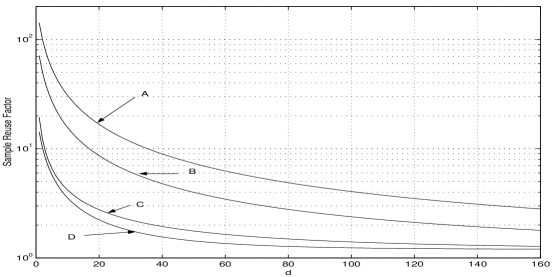
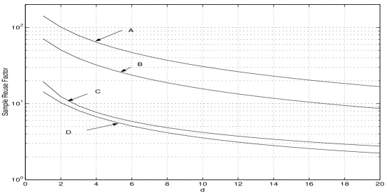
See the appendix for proof. For illustration purposes, we choose $r_{i}=b-\frac{(b-a)(i-1)}{l-1}$ for $i=1,2,\ldots,l$. By Theorem 1, ${\cal F}_{reuse}={l}/{l-\sum_{i=2}^{l}\left(1-\frac{1}{\frac{l-1}{1-\frac{a}{b}}-i+2}\right)^{d}}$. Figures 1 and  2 show that the improvement over the conventional approach is significant when $d$ is not large. These figures also reveal that the sample reuse factor does not scale well with the uncertainty dimension. For example, when $d>160$, the efficiency gained from sample reuse techniques may not be attractive.

Figure 1: Performance improvement (${\rm A:}\;l=200,\;b=2a;\;\;{\rm B:}\;l=100,\;b=2a;\;\;{\rm C:}\;l=100,\;a=0;\;\;{\rm D:}\;l=20,\;b=2a$).

Figure 2: Performance improvement (${\rm A:}\;l=200,\;b=2a;\;\;{\rm B:}\;l=100,\;b=2a;\;\;{\rm C:}\;l=100,\;a=0;\;\;{\rm D:}\;l=20,\;b=2a$).

5 Illustrative examples

In this section we demonstrate through examples the power of the sample reuse algorithm in solving a wide variety of complicated robustness analysis problems which are intractable in the classical deterministic framework.

First, we consider an example which has been studied in [11] by a deterministic approach. The system is as shown in Figure 3.

Figure 3: Uncertain system.

The compensator is $C(s)=\frac{s+2}{s+10}$ and the plant is $P(s)=\frac{800(1+0.1\delta_{1})}{s(s+4+0.2\delta_{2})(s+6+0.3\delta_{3})}$ with parametric uncertainty $\Delta=[\delta_{1},\delta_{2},\delta_{3}]^{\rm T}$. The nominal system is stable. The closed-loop roots of the nominal system are

$$z_{1}=-15.9178,\;\;z_{2}=-1.8309,\;\;z_{3}=-1.1256+7.3234i,\;\;z_{4}=-1.1256-7.3234i.$$

The $H_{\infty}$ norm of the nominal closed-loop transfer function is ${||T^{0}||}_{\infty}=2.78$. The peak value, rise time, and settling time of step response of the nominal system are, respectively, $P_{peak}^{0}=1.47,\;\;t_{r}^{0}=0.185,\;\mbox{{\rm and} }t_{s}^{0}=3.175$. In all of the following examples, we take $l=100$. To guarantee that the absolute error of the estimate for the proportion is less than $0.01$ with confidence level $99\%$, we choose $N=26,492$ based on the well-known Chernoff bound (see [12, 19] for “sharper” bounds). Since the Chernoff bound is conservative, we also performed a post-experimental evaluation of the estimates by constructing confidence intervals with confidence level $99\%$ based on Clopper–Pearson’s method [10].

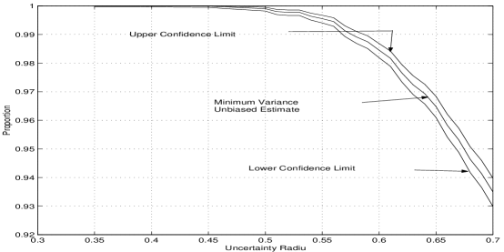
Figure 4 is the robustness degradation curve for robust stability over uncertainty set ${\cal B}_{\infty}(r):=\{\Delta:\;||\Delta||_{\infty}\leq r\}$. It demonstrates that a significant enhancement of the robustness margin can be achieved at the price of a small risk.

Figure 4: Robustness degradation curve (reuse factor $=41$).

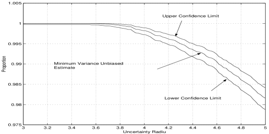
Figure 5 is the robustness degradation curve, with the robustness requirement ${\bf P}$ defined as stability and $H_{\infty}$ norm $<170\%\;{||T^{0}||}_{\infty}$, and the uncertainty set defined as the ellipsoid ${\cal B}_{2}(r):=\left\{\Delta:\;||\Delta||_{2}\leq r\right\}$.

Figure 5: Robustness degradation curve (reuse factor $=43$).

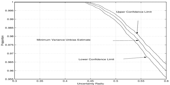
Figure 6 is the robustness degradation curve with the robustness requirement ${\bf P}$ defined as ${\cal D}$-stability with the domain of poles defined as: real part $<-1.5$, or it falls within one of the two disks centered at $z_{3}$ and $z_{4}$ with radius $0.3$. The uncertainty set is defined as the polytope

$${\cal B}_{H}(r):=\left\{r\Delta+(1-r)\;\frac{\sum_{i=1}^{4}\Delta^{i}}{4}:\Delta\in{\rm conv}\{\Delta^{1},\Delta^{2},\Delta^{3},\Delta^{4}\}\right\},$$

where “conv” denotes the convex hull of $\Delta^{i}=[\frac{1}{2}\sin(\frac{2i-1}{3}\pi),\;\frac{1}{2}\cos(\frac{2i-1}{3}\pi),\;-\frac{\sqrt{3}}{2}]^{\rm T}$ for $i=1,2,3$ and $\Delta^{4}=[0,\;0,\;1]^{\rm T}$.

Figure 6: Robustness degradation curve (reuse factor $=49$).

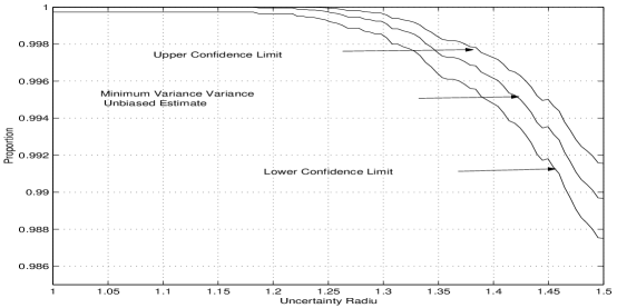
Figure 7 is the robustness degradation curve for the case where the uncertainty set is ${\cal B}_{\infty}(r):=\{\Delta:\;||\Delta||_{\infty}\leq r\}$, the robustness requirement ${\bf P}$ is: stability, and rise time $t_{r}<135\%\;t_{r}^{0}=0.25$, settling time $t_{s}<110\%\;t_{s}^{0}=3.5$, and overshoot $P_{peak}<116\%\;P_{peak}^{0}=1.7$.

Figure 7: Robustness degradation curve (reuse factor $=38$).

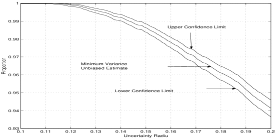
Finally, we consider the same example in [8] where the class of uncertainty is defined as

$${\bf\Delta}:=\{{\rm blockdiag}[q_{1}I_{5},\;q_{2}I_{5},\;\Delta_{1}]\},$$

where $\Delta_{1}\in{\bf C}^{4\times 4}$, and $I_{5}$ denotes the identity matrix of $5\times 5$. By Theorem 1, we have $d=34$. Figure 8 shows the robustness degradation curve. An improvement (of efficiency) about fivefold is achieved by our algorithm.

Figure 8: Robustness degradation curve (reuse factor $=5$).

6 A probabilistic perspective

In sections 2 and 3, we have derived our sample reuse algorithm from the worst-case deterministic framework. In this section, we show that the proposed algorithm is also applicable from the perspective of the random nature of uncertainty. In situations where we need to take into account the random nature of uncertainty, the pioneering work of Barmish, Lagoa, Tempo, Bai, and Fu [2, 1] allows our sample reuse algorithm to be applied to solve efficiently a wide variety of robustness problems. The following theorem plays an important role.

Theorem 2 (see [2])

Suppose that uncertainty ${\bf\Delta}$ is a random variable with a density function $f(\Delta)$ which depends only on $\ell(\Delta)$ and is nonincreasing with respect to $\ell(\Delta)$. Then

$$\Pr\{{\rm The\;associated\;system}\;G({\bf\Delta})\;{\rm guarantees}\;{\bf P}\;\;|\;\;{\bf\Delta}\in{\cal B}(r)\}\geq\inf_{0\leq\rho\leq r}\mathbb{P}(\rho).$$

Remark 1. A remarkable fact of Theorem 2 is that no assumption needs to be imposed on the robustness requirement ${\bf P}$. The assumption in Theorem 2 is roughly interpreted to mean that the probability measure of the uncertainty is radially symmetrical with respect to the nominal value. In many applications, small perturbations are more likely than large perturbations, and the uncertainty is sufficiently unstructured so as to be treated equally likely in the surface of ${\cal B}(r)$ [2].

Remark 2. It should be noted that Theorem 2 applies to a homogeneous star-shaped bounding set, $l_{p}$ ball, and spectral norm ball. We introduce in Theorem 2 a conditional probability based on the following reason: It does not seem logical to treat the uncertainty as different bounded random variables. For example, if the uncertainty possesses a certain distribution over ${\cal B}(r_{1})$, it would be a contradiction that the uncertainty possesses another distribution over ${\cal B}(r_{2})$ for $r_{2}>r_{1}$. In fact, if the uncertainty is of random nature, then the associated distribution is unique.

Based on Theorem 2, we can apply the sample reuse algorithm to estimate $\mathbb{P}(r)$ for $r\in[0,b]$, from which we can construct the lower bounds for $\Pr\{G({\bf\Delta})\;{\rm guarantees}\\ \;{\bf P}\;\;|\;\;{\bf\Delta}\in{\cal B}(r)\}$.

7 Conclusion

We develop a fast algorithm for computing the robustness degradation function which overcomes the computational complexity and conservatism issue of the deterministic worst-case methods. We also demonstrate that our algorithm can provide efficient solutions for a wide variety of robustness analysis problems which are intractable by the deterministic worst-case methods. We derive our algorithm from the worst-case deterministic framework and also show that the algorithm is applicable from a probabilistic perspective.

Appendix A Proof of Theorem 1

The following lemma follows essentially from the definition of volume function ${\rm vol}(.)$.

Lemma 1

Let $X=\{\Delta\in{\bf C}^{n\times m}:\bar{\sigma}(\Delta)\leq r\}$ and $Y=\{\Delta\in{\bf C}^{m\times n}:\bar{\sigma}(\Delta)\leq r\}$. Let $Z=\{\Delta\in{\bf R}^{n\times m}:\bar{\sigma}(\Delta)\leq r\}$ and $W=\{\Delta\in{\bf R}^{m\times n}:\bar{\sigma}(\Delta)\leq r\}$. Then ${\rm vol}(X)={\rm vol}(Y)$ and ${\rm vol}(Z)={\rm vol}(W)$.

Lemma 2

Let $m\geq n$. Define spectral norm ball ${\cal B}_{\sigma}^{C}(r)=\{\Delta\in{\bf C}^{n\times m}:\bar{\sigma}(\Delta)\leq r\}$ and spectral norm ball ${\cal B}_{\sigma}^{R}(r)=\{\Delta\in{\bf R}^{n\times m}:\bar{\sigma}(\Delta)\leq r\}$. Then ${\rm vol}({\cal B}_{\sigma}^{C}(r))={\rm vol}({\cal B}_{\sigma}^{C}(1))r^{d}$ with $d=2mn$ and ${\rm vol}({\cal B}_{\sigma}^{R}(r))={\rm vol}({\cal B}_{\sigma}^{R}(1))r^{d}$ with $d=mn$.

Proof.

By Theorem 1 of [8], we have

$$\frac{\Upsilon_{C}}{{\rm vol}({\cal B}_{\sigma}^{C}(r))}\;\int_{r\geq\sigma_{1}>\sigma_{2}>\cdots>\sigma_{n}>0}\prod_{i=1}^{n}\sigma_{i}^{2(m-n)+1}\times\prod_{1\leq i<k\leq n}(\sigma_{i}^{2}-\sigma_{k}^{2})^{2}\;d\sigma_{1}d\sigma_{2}\cdots d\sigma_{n}=1\\$$

with $\Upsilon_{C}=\frac{2^{n}\pi^{mn}}{\prod_{k=1}^{n}(n-k)!(m-k)!}$. Performing a change of variables with $x_{i}=\frac{\sigma_{i}}{r}$ for $i=1,\ldots,n$, we have

$$\frac{r^{2mn}\Upsilon_{C}}{{\rm vol}({\cal B}_{\sigma}^{C}(r))}\;\int_{1\geq x_{1}>x_{2}>\cdots>x_{n}>0}\prod_{i=1}^{n}x_{i}^{2(m-n)+1}\\ \times\prod_{1\leq i<k\leq n}(x_{i}^{2}-x_{k}^{2})^{2}\;dx_{1}dx_{2}\cdots dx_{n}=1.$$

Thus

$${\rm vol}({\cal B}_{\sigma}^{C}(1))=\Upsilon_{C}\int_{1\geq x_{1}>x_{2}>\cdots>x_{n}>0}\prod_{i=1}^{n}x_{i}^{2(m-n)+1}\times\prod_{1\leq i<k\leq n}(x_{i}^{2}-x_{k}^{2})^{2}\;dx_{1}dx_{2}\cdots dx_{n},$$

and

$${\rm vol}({\cal B}_{\sigma}^{C}(r))={\rm vol}({\cal B}(1))\;r^{2mn}.$$

Similarly, by Theorem 2 of [8], we can show that ${\rm vol}({\cal B}_{\sigma}^{R}(r))={\rm vol}({\cal B}_{\sigma}^{R}(1))r^{d}$ with $d=mn$.    $\Box$

Lemma 3

${\rm vol}({\cal B}(r))={\rm vol}({\cal B}(1))r^{d}$ where $d=n$ for $l_{p}$ ball ${\cal B}_{p}(r)$ and homogeneous star-shaped bounding set ${\cal B}_{H}(r)$; and $d=\sum_{i=1}^{s}\kappa(q_{i})+\sum_{j=1}^{c}\kappa(\Delta_{j})$ for spectral norm ball ${\cal B}_{\sigma}(r)$.

Proof.

The truth is obvious for cases of an $l_{p}$ ball and homogeneous star-shaped bounding set. To prove the lemma for the case of a spectral norm ball, we need to apply Lemmas 1 and 2.    $\Box$

Lemma 4

For $i=1,\ldots,l-1$,

$${\cal E}\left[{\bf n}_{i+1}\right]=N-\sum_{j=1}^{i}\left(\frac{r_{i+1}}{r_{j}}\right)^{d}\;{\cal E}\left[{\bf n}_{i}\right].$$

Proof.

Let $q^{1},q^{2},\ldots,q^{{\bf n}_{j}}$ be the samples generated on $r_{j}$. For $l=1,\ldots,{\bf n}_{j}$, define binomial random variable $X_{j,i+1}^{l}$ such that

$$X_{j,i+1}^{l}:=\left\{\begin{array}[]{ll}1\;\;\;{\rm if}\;q^{l}\;{\rm fall\;in}\;{\cal B}(r_{i+1}),\\ 0\;\;\;\;{\rm otherwise.}\end{array}\right.$$

By the rule of the sample reuse algorithm,

$$N={\bf n}_{i+1}+\sum_{j=1}^{i}\sum_{l=1}^{{\bf n}_{j}}X_{j,i+1}^{l}.$$

Thus for $i=1,\ldots,l-1$,

$${\cal E}\left[{\bf n}_{i+1}\right]=N-\sum_{j=1}^{i}{\cal E}\left[\sum_{l=1}^{{\bf n}_{j}}X_{j,i+1}^{l}\right]=N-\sum_{j=1}^{i}\sum_{n\in\Omega_{{\bf n}_{j}}}\sum_{l=1}^{n}{\cal E}\left[X_{j,i+1}^{l}\;|\;{\bf n}_{j}=n\right]\;\Pr\{{\bf n}_{j}=n\},$$

where $\Omega_{{\bf n}_{j}}$ denotes the sample space of ${\bf n}_{j}$. Since $q^{l}$ is a random variable with uniform distribution over ${\cal B}(r_{i})$, it follows from Lemma 3 that

$${\cal E}[X_{j,i+1}^{l}\;|\;{\bf n}_{j}=n]=\frac{{\rm vol}({\cal B}(r_{i+1}))}{{\rm vol}({\cal B}(r_{j}))}=\left(\frac{r_{i+1}}{r_{j}}\right)^{d}.$$

Therefore,

$${\cal E}\left[{\bf n}_{i+1}\right] = N-\sum_{j=1}^{i}\sum_{n\in\Omega_{{\bf n}_{j}}}n\;\left(\frac{r_{i+1}}{r_{j}}\right)^{d}\;\Pr\{{\bf n}_{j}=n\}$$

$$= N-\sum_{j=1}^{i}\;\left(\frac{r_{i+1}}{r_{j}}\right)^{d}\;\sum_{n\in\Omega_{{\bf n}_{j}}}n\Pr\{{\bf n}_{j}=n\}$$

$$= N-\sum_{j=1}^{i}\left(\frac{r_{i+1}}{r_{j}}\right)^{d}\;{\cal E}\left[{\bf n}_{i}\right].$$

$\Box$

Lemma 5

For $i=2,\cdots,l$,

$${\cal E}\left[{\bf n}_{i}\right]=N-N\left(\frac{r_{i}}{r_{i-1}}\right)^{d}.$$

Proof.

We use induction. Obviously,

$${\cal E}\left[{\bf n}_{1}\right]=N.$$

By Lemma 4, we get

$${\cal E}\left[{\bf n}_{2}\right]=N-N\left(\frac{r_{2}}{r_{1}}\right)^{d}.$$

Suppose it is true that

$${\cal E}\left[{\bf n}_{i}\right]=N-N\left(\frac{r_{i}}{r_{i-1}}\right)^{d}.$$

Then

$$\sum_{j=1}^{i}\;\left(\frac{r_{i+1}}{r_{j}}\right)^{d}\;{\cal E}\left[{\bf n}_{j}\right] = \sum_{j=1}^{i}\left(\frac{r_{i+1}}{r_{j}}\right)^{d}\;\left[N-N\left(\frac{r_{j}}{r_{j-1}}\right)^{d}\right]$$

$$= \sum_{j=1}^{i}\left[N\left(\frac{r_{i+1}}{r_{j}}\right)^{d}-N\left(\frac{r_{i+1}}{r_{j-1}}\right)^{d}\right]$$

$$= N\left(\frac{r_{i+1}}{r_{i}}\right)^{d}.$$

It follows from Lemma 4 that

$${\cal E}\left[{\bf n}_{i+1}\right]=N-\sum_{j=1}^{i}\;\left(\frac{r_{i+1}}{r_{j}}\right)^{d}\;{\cal E}\left[{\bf n}_{j}\right]=N-N\left(\frac{r_{i+1}}{r_{i}}\right)^{d}.$$

The proof of Lemma 5 is thus completed by induction.    $\Box$

Now we are in the position to prove Theorem 1. By Lemmas 4 and 5, we have

$${\cal E}\left[\sum_{i=1}^{l}{\bf n}_{i}\right]=N+\sum_{i=2}^{l}\left[N-N\left(\frac{r_{i}}{r_{i-1}}\right)^{d}\right]=Nl-N\;\sum_{i=2}^{l}\left[1-\left(\frac{r_{i}}{r_{i-1}}\right)^{d}\right].$$

Therefore,

$${\cal F}_{reuse}=\frac{Nl}{{\cal E}[\sum_{i=1}^{l}{\bf n}_{i}]}=\frac{l}{l-\sum_{i=2}^{l}\left(\frac{r_{i}}{r_{i-1}}\right)^{d}}$$

and thus the proof of Theorem 1 is completed.

References

- [1] E. W. Bai, R. Tempo, and M. Fu, Worst-case properties of the uniform distribution and randomized algorithms for robustness analysis, Math. Control Signals Systems, 11 (1998), pp. 183–196.
- [2] B. R. Barmish, C. M. Lagoa, and R. Tempo, Radially truncated uniform distributions for probabilistic robustness of control systems, in Proceedings of American Control Conference, Albuquerque, NM, American Automatic Control Council, 1997, pp. 853–857.
- [3] B. R. Barmish, A probabilistic result for a multilinearly parameterized norm, in Proceedings of American Control Conference, Chicago, IL, American Automatic Control Council, 2000, pp. 3309–3310.
- [4] B. R. Barmish and B. T. Polyak, A new approach to open robustness problems based on probabilistic predication formulae, in Proceedings of the IFAC World Congress, Vol. H, San Francisco, CA, International Federation of Automatic Control, 1996, pp. 1–6.
- [5] B. R. Barmish and C. M. Lagoa, The uniform distribution: A rigorous justification for its use in robustness analysis, Math. Control Signals Systems, 10 (1997), pp. 203–222.
- [6] X. Chen and K. Zhou, Order statistics and probabilistic robust control, Systems Control Lett., 35 (1998), pp. 175–182.
- [7] X. Chen and K. Zhou, Constrained robustness analysis and synthesis by randomized algorithms, IEEE Trans. Automat. Control, 45 (2000), pp. 1180–1186.
- [8] G. Calafiore, F. Dabbene, and R. Tempo, Randomized algorithms for probabilistic robustness with real and complex structured uncertainty, IEEE Trans. Automat. Control, 45 (2000), pp. 2218–2235.
- [9] G. Calafiore, F. Dabbene, and R. Tempo, Radial and uniform distributions in vector and matrix spaces for probabilistic robustness, in Topics in Control and Its Applications, D. Miller and L. Qiu, eds., Springer-Verlag, London, 1999, pp. 17–31.
- [10] C. J. Clopper and E. S. Pearson, The use of confidence or fiducial limits illustrated in the case of the binomial, Biometrika, 26 (1934), pp. 404–413.
- [11] R. R. De Gaston and M. G. Safonov, Exact calculation of the multiloop stability margin, IEEE Trans. Automat. Control, 33 (1988), pp. 156–171.
- [12] P. P. Khargonekar and A. Tikku, Randomized algorithms for robust control analysis and synthesis have polynomial complexity, in Proceedings of the 35th Conference on Decision and Control, Kobe, Japan, IEEE Control Systems Society, 1996, pp. 3470–3475.
- [13] C. M. Lagoa, Probabilistic enhancement of classic robustness margins: A class of non-symmetric distributions, in Proceedings of American Control Conference, Chicago, IL, American Automatic Control Council, 2000, pp. 3802–3806.
- [14] C. Marrison and R. F. Stengel, Robust control system design using random search and genetic algorithms, IEEE Trans. Automat. Control, 42 (1997), pp. 835–839.
- [15] S. R. Ross and B. R. Barmish, Distributionally robust gain analysis for systems containing complexity, in Proceedings of the 40th Conference on Decision and Control, Orlando, FL, IEEE Control Systems Society, 2001, pp. 5020–5025.
- [16] L. R. Ray and R. F. Stengel, A Monte Carlo approach to the analysis of control system robustness, Automatica J. IFAC, 3 (1993), pp. 229–236.
- [17] R. F. Stengel and L. R. Ray, Stochastic robustness of linear time-invariant systems, IEEE Trans. Automat. Control, 36 (1991), pp. 82–87.
- [18] B. T. Polyak and P. S. Scherabakov, Random spherical uncertainty in estimation and robustness, IEEE Trans. Automat. Control, 45 (2000), pp. 2145–2150.
- [19] R. Tempo, E. W. Bai, and F. Dabbene, Probabilistic robustness analysis: Explicit bounds for the minimum number of samples, Systems Control Lett., 30 (1997), pp. 237–242.
- [20] R. Tempo and F. Dabbene, Probabilistic robustness analysis and design of uncertain systems, in Dynamical Systems, Control, Coding, Computer Vision, Progr. Systems Control Theory 25, G. Picci, ed., Birkhäuser, Basel, 1999, pp. 263–282.
- [21] M. Vidyasagar and V. D. Blondel, Probabilistic solutions to NP-hard matrix problems, Automatica J. IFAC, 37 (2001), pp. 1597–1405.
- [22] M. Vidyasagar, Randomized algorithms for robust controller synthesis using statistical learning theory, Automatica J. IFAC, 37 (2001), pp. 1515–1528.