Ergodicity and Central Limit Theorem in Systems with Long-Range Interactions
Abstract
In this letter we discuss the validity of the ergodicity hypothesis in theories of violent relaxation in long-range interacting systems. We base our reasoning on the Hamiltonian Mean Field model and show that the life-time of quasi-stationary states resulting from the violent relaxation does not allow the system to reach a complete mixed state. We also discuss the applicability of a generalization of the central limit theorem. In this context, we show that no attractor exists in distribution space for the sum of velocities of a particle other than the Gaussian distribution. The long-range nature of the interaction leads in fact to a new instance of sluggish convergence to a Gaussian distribution.
pacs:
02.50.-r; 05.20.Dd; 05.90.+mI Introduction
Physical systems with long-range interaction has been widely studied with results reported in the literature, and properties that are markedly different from short range interacting systems, e.g, non-Gaussian quasi-stationary states, negative heat-capacity, temperature jumps at critical points, anomalous diffusion and ensemble inequivalence newproc ; oldproc . Examples include self-gravitating systems, vortices in two-dimensional fluids, dipolar interactions, fractures in solids and simplified models as the Hamiltonian Mean Field (HMF), free electron laser and the plasma single wave models oldproc ; chavanis2 ; sire ; hmforig ; felmod ; tennyson . The nature of the non-Gaussian quasi-stationary states arising from the dynamics can be interpreted as stable stationary states of the mean-field Vlasov equation which describes the system in the limit , where is the number of particles r11 ; r12 . This equivalence was explicitly verified by comparing results from direct simulations of a hamiltonian system and the numerical solutions of the associated Vlasov equation antoniazzi . For longer times correlations build between particles and the Vlasov equation must be replaced by a proper kinetic equation chavanis ; binney . The initial stage of time evolution is called violent relaxation and corresponds to a very rapid evolution from the initial condition into a quasi-stationary state. Since the seminal paper by Lynden-Bell lyndenbell , many attempts were made to formulate the statistical mechanics of violent relaxation (see for instance References arad and 18c and references therein), but a satisfactory theory for predicting the outcome of the violent relaxation process is still lacking.
In the last decade many papers tried to identify the outcome states of a violent relaxation with the q-Gaussian distributions:
| (1) |
arising from the maximization of the Tsallis entropy latora ; latora2 ; pluchino ; pluchino2 . Nevertheless some authors pointed out that this approach is too limited in scope, since q-Gaussian are too specific to handle the richness of quasi-stationary states observed in long-range interacting systems nos1 ; 18b ; 18c ; 18d . More recently some effort was made to generalize the Central Limit Theorem (CLT). It was shown that for a special type of correlation (called q-independence) the sum of stochastic variables tend to a q-Gaussian distribution umarov ; tsallis1 ; queiros . Some attempts were made to provide specific examples where such type of behavior occur tirnakli ; moyano ; pluchino3 ; pluchino4 ; 25b ; 25c ; ernesto ; 32 . In a recent paper Hilhorst and Schehr hilhorst have shown analytically that the sum of correlated stochastic variables for two such examples (see Ref. moyano and Reference 12 of hilhorst ) are in fact not q-Gaussians, but functions that are only approximated by q-Gaussians. Dauxois also raised some additional points on the applicability of this approachdauxois ; tsallis2 . Rodriguez and collaborators described a simple model with scale invariance where this generalized CLT indeed applies rodrigues . This shows that examples satisfying its hipothesis are difficult to obtain. In this work we are interested to study the sum of stochastic variables given by the momenta of particles in a classical long-range interacting system, the HMF model pluchino3 ; pluchino4 ; ernesto , and possible relationships with the generalization of the CLT, and to ergodicity.
The HMF model is a paradigmatic and well-studied model, displaying many characteristics of long-range interacting systems. In references it is argued, based on numerical simulations, that the q-generalized CLT is realized in the sum of velocities of particles of the HMF model. On this basis it was also argued that the system is non-ergodic. Pluchino and co-workers refined this assertion by pointing out that q-Gaussians are only obtained in some realizations of their numerical simulations (depending on the microscopic details of the initial conditions), while in the remaining cases the distributions are either Gaussian or a sort of intermediate function between Gaussians and q-Gaussians 32 . In this paper we show that if an attractor ever exists in the distribution space it is a Gaussian. The distributions obtained in the conditions used in references pluchino3 ; pluchino4 ; ernesto ; 32 are neither q-Gaussians nor limit distributions in the sense of a genuine CLT.
We also discuss that the time averages over a single particle history and ensemble averages are different, albeit diminishing with time. This leads to the conclusion that even-though the system becomes more ergodic (mixed), the quasi-stationary state relaxes to the final thermodynamic equilibrium before the ergodicity condition is reached. This explains the failure of Lynden-Bell theory of violent relaxation, which requires a complete mixing state.
II Central limit theorem and long-range interactions - The HMF model
Let us start by writing down the hamiltonian for the HMF model hmforig :
| (2) |
This model describes a system of rotors with angular positions and angular momenta (velocities) . The magnetization is defined as the average value of the modulus of the vector :
| (3) |
The classical central limit theorem states that the sum of non-correlated stochastic variables with finite standard deviation converges to a Gaussian distribution. The standard deviation of the summed variable scales with levi . Let us then consider the discrete time average momentum of a fixed particle in a system with particles, say the -th particle:
| (4) |
where is a fixed time interval. This average is also a stochastic variable when considering its values for each of the particles in the system. If is sufficiently large so that the momenta of the same particle at different times are not correlated, and for statistically stationary states, the standard deviation scales as . Due to the mean-field nature of the system, all relevant physical quantities can be obtained from the one-particle distribution function . If the standard deviation of approaches zero for large enough , then computing averages using is equal to time-averages over one single particle evolution, i. e. the system is said to be ergodic. For the purposes of the discussion below and for comparison with other works, we also define the reduced average momentum (vanishing average and unit standard deviation) by:
| (5) |
where is the standard deviation of :
| (6) |
and
| (7) |
which vanishes for systems with zero total momentum. A (central) limit exists for the sum of stochastic variables if the ensuing distribution has a limit, or rephrasing, if any finite statistical moment has a limit for which then corresponds to the moment of the limit distribution. This is the meaning of the word limit in the name of such theorems. Reduced variables are useful for comparing distribution functions with different averages or dispersions, but which are of the same type, e. g. all Gaussian distributions are the same with respect to the reduced variable. Let us note that unfortunately contrary to what is stated in Ref. pluchino3 , ergodicity is not equivalent to requiring that the distribution of each single and the reduced distribution of the momenta are the same. As a counter example, consider a system which randomly jumps between two states represented by or . The state of the system after the -th jump is labeled by the random variable . The distribution of probabilities after a large number of jumps converge to . Since the variables are uncorrelated and have finite standard deviations, the sum , approaches a Gaussian distribution as increases, which is obviously different from the distribution for . Clearly this does not imply that the system is non-ergodic, as this is a very simple case of an ergodic system (time averages are equal to ensemble averages). Therefore arguing that a fixed time reduced distribution of velocities different from the distribution of the summed variable as defined in eq. (5) implies non-ergodicity is not correct. We show below that for long-range interacting systems the dispersion in scales much slower than , even at thermodynamical equilibrium, due to the presence of strong velocity auto-correlations. If the life-time of the quasi-stationary state is shorter than the time required for in eq. (6) to significantly approach zero, then the assumption of ergodicity used in Lynden-Bell theory breaks down. In the present paper we study this issue in numerical simulations of the HMF model.
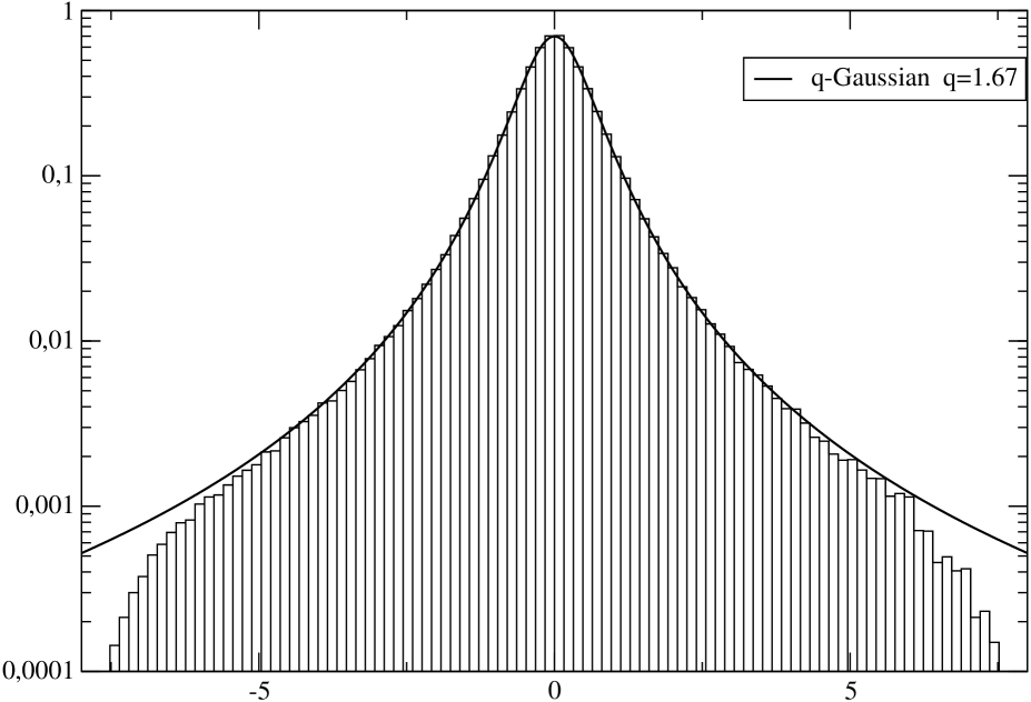
We first consider the issue of whether a limit distribution exists for the reduced variable , and if so if it is a q-Gaussian, as claimed in Refs. pluchino3 ; pluchino4 ; ernesto ; 32 . In order to extend the analysis of distributions we perform numeric simulations using the parameter values of pluchino3 ; pluchino4 ; ernesto but improving statistical precision. Let us consider the case studied in Ref. pluchino3 with the following parameters: , and , with a transient time to allow the system to reach the quasi-stationary state, with all particles at the origin (magnetization ) and the momenta uniformly distributed in an interval , with an energy per particle . The simulations were performed using a fourth-order simpletic integrator yoshida , the same as in pluchino3 , and repeated using a different simpletic integrator for checking 30b . The maximum relative energy error admitted was , and we average over 10,000 realizations (10 times more than in pluchino3 ), which gives a much better statistical accuracy in the tails of the distribution. At this point we note that the use of a good quality random number generator is strongly required to avoid unwanted correlations when generating the initial conditions. For a good discussion of this point see 33 ; 34 . The resulting distribution for is shown in the upper panel of figure 1, together with the best fitted q-Gaussian with (the value obtained in pluchino3 is ). It is clear from the tails of the distribution that it is not a q-Gaussian. The lower panel in figure 1 shows the reduced velocity distribution function at time (the final time of the interval over which the sum (5) runs), which coincides with the one obtained in pluchino3 . This distribution is not Gaussian and can be well approximated as a limit case of a Lynden-Bell distribution for a two-level initial distribution for (see eq. (9) below). It is straightforward to show that the distribution of cannot be a q-Gaussian from the fact that for the statistical moments of the reduced variables :
| (8) |
diverge for for some . In fact eq. (8) is an approximation from the simulations for the true moments obtained for . If the true value of diverges, then computing the simulation value of from eq. (8) for increasing would show no convergence to a finite value. Nevertheless in all our simulations the value of always converged to a finite value for a given such that the corresponding fitted q-Gaussian implied an infinite value.
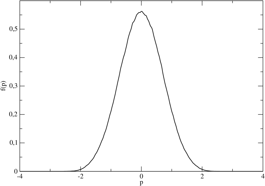
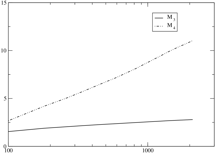
Another important point is that the situation at the final time is not a limit state, i. e. the moments of the reduced variable do not converge to a constant value for increasing time, as seen in fig. 2. Along these lines, for the situation considered in pluchino3 no limit distribution is obtained.
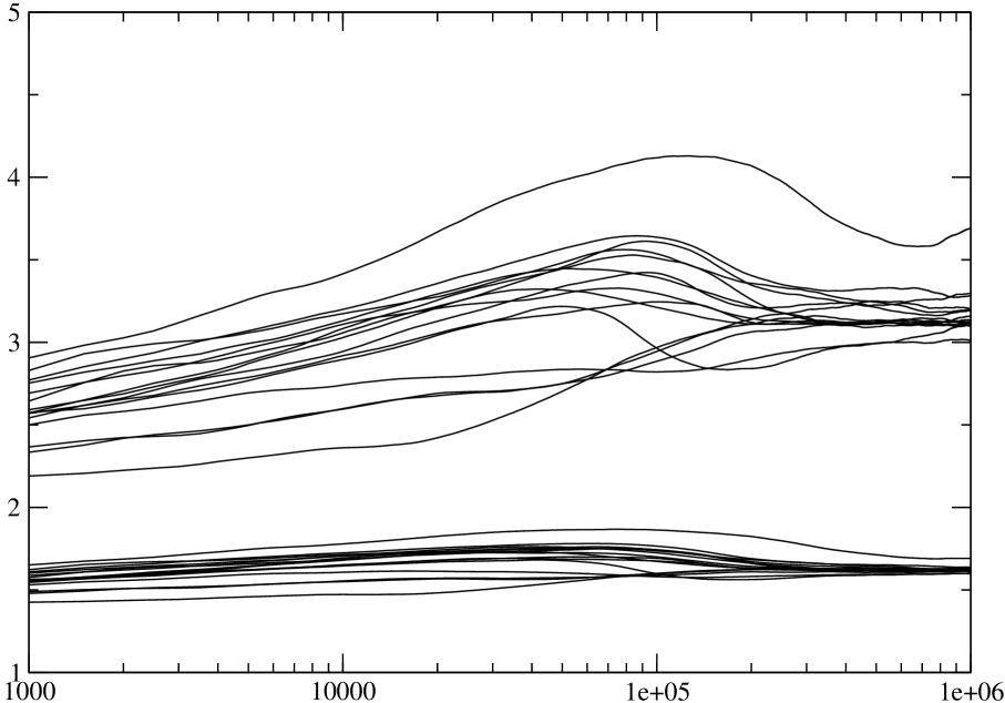
Extending our analysis let us consider the case studied in ref. pluchino4 , with , , and , with 50 realizations and the same type of initial conditions. The results are shown if fig. 3, together with the q-Gaussian fit with smallest error. It is evident from the figure that no q-Gaussian is realized. The lower panel in fig. 3 shows the moments and for 15 different realizations as function of time. The reference values of the moments for a reduce variable having a Gaussian distribution are and . The figure shows that all cases, except one which is far from a limit situation, are converging to a Gaussian distribution. The present case is an example of sluggish convergence of a stochastic process to a Gaussian, as discussed in a different context in References annibal ; manteiga . The convergence rate itself depends on the details of the initial conditions.

From the results presented above we can draw the following conclusions: the only true attractor observed in distribution space for the sum in eq. (5) is the Gaussian distribution. In all cases considered here and in tsallis1 ; queiros the distribution is never a q-Gaussian. The only situation where a limit exists for the distribution of the sum variable is such that it converges to a Gaussian, as show by the time evolution of moments. The claim that a generalized central limit theorem leading to a Tsallis distribution is observed for the HMF model is therefore invalidated. This do not precludes the applicability of such theorem in other situations.
III Non-ergodic behavior
Now we turn to the ergodicity problem for this system. As explained above, we look at the time evolution of the dispersion in eq. (6). We consider the HMF model with particles, , with a uniform initial distribution in an interval given by , if ; , and zero otherwise. The parameters and can be used to adjust the energy and initial magnetization. The predicted final state being computed using the procedure described in Ref. afbcdr . In that direction we first note that the value in eq. (3) in the quasi-stationary state can be set to zero by a global shift in the angles. The distribution function of the quasi-stationary state predicted by Lynden-Bell theory for an initial distribution with two levels ( and zero) is given by lyndenbell :
| (9) |
where
| (10) |
is the one particle energy, and and are Lagrange multipliers determined from the energy and normalization constraints:
| (11) |
| (12) |
together with the corresponding expression for :
| (13) |
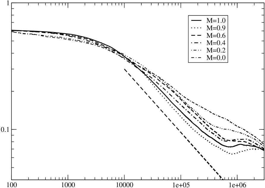
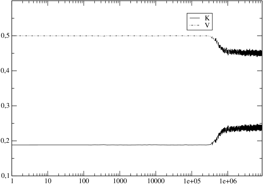
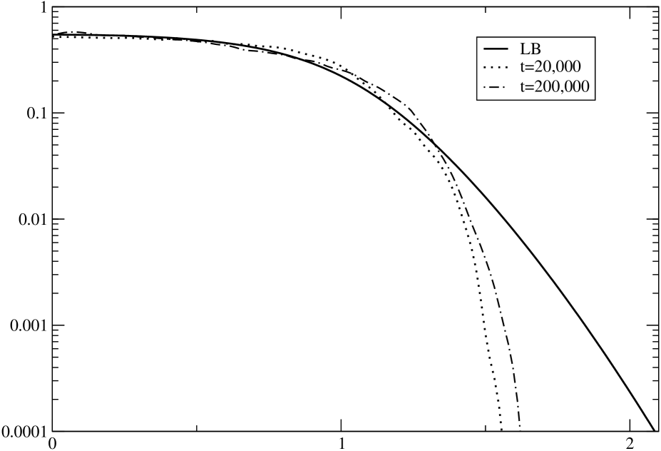
Equations (11) and (12) form an algebraic system in the unknowns and and can be solved numerically to explicitly determine . Is is thoroughly discussed in the literature that the predictions of Lynden-Bell theory yield at best approximate results due to incomplete mixing. We will show that this is in fact due to the strong velocity auto-correlation which prevents the system to reach an ergodic state, in the sense discussed above. We show in fig. 4 the dispersion (standard deviation) for the summed variable for some values of the magnetization of the initial state for . The life-time of the quasi-stationary state can be inferred from fig. 5 showing the kinetic and potential energies per particle for the case (the other cases has essentially the same life-time) as . The scaling for is reached only after a very long time, of the order of the life-time of the stationary state. The system evolves to the thermodynamical equilibrium well before the dispersion can attain a significantly small value. Figure 6 shows the velocity distribution function for two times compared with the Lynden-Bell distribution function for . Even though the distribution is slowly approaching the theoretical prediction while decreases, the difference remains always significant.
IV Concluding Remarks
We have shown that the HMF model is non-ergodic due to strong auto-correlations in particle velocities, which are also responsible for anomalous diffusion and Levi walks, restraining the dispersion in the time average of the velocity of each particle to approach zero before the system finally settles down in its thermodynamical equilibrium. The system has not enough time to reach ergodicity and therefore any intermediate state before final equilibrium is incompletely relaxed. Ergodicity is only fulfilled for asymptotic times, well after thermodynamic equilibrium occurs. This clearly points out that a solution of the violent relation problem must necessarily rely on a dynamical theory, based for instance in the solution of a proper kinetic equation as already pointed out by Chavanis 18c . Many of the points presented here can be extended to other systems with long-range interactions as long as strong velocity auto-correlations are present. We have also shown, if simulations are performed with care to statistical precision, that the only attractor observed for the sum of the velocity of a single particle at fixed time intervals is the Gaussian distribution, thus invalidating the claims by Tsallis and collaborators that such attractors should be q-Gaussian distributions.
V Acknowledgments
The authors thanks C. Tsallis for useful discussions. This work was partially financed by CNPq (Brazil).
References
- (1) Dynamics and Thermodynamics of Systems With Long Range Interactions: Theory and Experiments, Eds. A. Campa, A. Giansanti, G. Morigi and F. F. Labini, AIP Conference Proceedings, Vol 970, (Melville, 2007).
- (2) Dynamics and Thermodynamics of Systems with Long Range Interaction, Eds. T. Dauxois, S. Ruffos and M. Wilkens, Lecture Notes in Physics Vol 602 (Berlin, 2002).
- (3) M. Antoni and S, Ruffo, Phys. Rev. E 52 (1995) 2361.
- (4) J. L. Tennyson, J, D. Meiss and P. J. Morrison, Physica D 71 (1994) 1.
- (5) P. H. Chavanis, Phys. Rev. Lett. 84 (2000) 5512.
- (6) P. H. Chavanis and C. Sire, Phys. Fluids. 13 (2001) 71804.
- (7) R. Bonifacio, F. Casagrande, G. Cerchioni, L. De Salvo Souza, P. Pierini and N. Piovella, Riv. Nuovo Cimento 13 (1990) 1.
- (8) W. Braun and K. Hepp, Commun. Math. Phys. 56 (1977) 101.
- (9) P. H. Chavanis, Physica A 361 (2006) 55.
- (10) A. Antoniazzi, F. Califano, D. Fanelli and S. Ruffo, Phys. Rev. Lett. 98 (2007) 150602.
- (11) P. H. Chavanis Physica A 387 (2008) 1504.
- (12) J. Binney and S. Tremaine, Galactic Dynamics Princeton Univ. Press, (Princeton, 1987).
- (13) D. Lynden-Bell, MNRAS 136 (1967) 101.
- (14) I. Arad and P. H. Johanson, MNRAS 363 (2005) 252.
- (15) P. H. Chavanis, Physica A 365 (2006) 102.
- (16) V. Latora, A. Rapisarda and C. Tsallis, Phys. Rev. E 64 (2001) 056134.
- (17) V. Latora, A. Rapisarda and C. Tsallis C., Physica A 305 (2002) 129.
- (18) A. Pluchino, V. Latora and A. Rapisarda, Physica D 193 (2004) 315.
- (19) A. Pluchino, V. Latora and A. Rapisarda, Cont. Mech. Therm. 16A. (2004) 245.
- (20) T. M. Rocha Filho, A. Figueiredo and M. A. Amato, Phys. Rev. Lett. 95 (2005) 190601.
- (21) P. H. Chavanis, Physica A 359 (2006) 177.
- (22) C. Féron and J. Hjorth, astro-ph/0801.2504.
- (23) S. Umarov, C. Tsallis and S. Steinberg, Milan J. Math. 76 (2008) DOI: 10.1007/s00032-008-0087-y. cond-mat/0603593.
- (24) C. Tsallis and S. M. D. Queiros, AIP Conf. Proc. 965 (2007) 8.
- (25) S. M. D. Queiros and C. Tsallis, AIP Conf. Proc. 965 (2007) 21.
- (26) U. Tirnakli, C. Beck and C. Tsallis, Phys. Rev. E 75 (2007) 040106(R).
- (27) L. G. Moyano, C. Tsallis, and M. Gell-Man, Europhys. Lett. 73 (2006) 813.
- (28) C. Tsallis, Physica A 365 (2006) 7.
- (29) J. A. Marsh, A. M. Fuentes, L. G. Moyano and C. Tsallis, Physica A 372 (2006) 183.
- (30) A. Pluchino, A. Rapisarda and C. Tsallis, Europhys. Lett. 80 (2007) 26002.
- (31) Pluchino A. Rapisarda A. cond-mat/0712.2539.
- (32) C. Tsallis, A. Rapisarda, A. Pluchino and E. P. Borge, Physica A 381 (2007) 143.
- (33) A. Pluchino, A. Rapisarda and C. Tsallis, cond-mat/0801.1914.
- (34) H. J. Hilhorst and G. Schehr, J. Stat. Mech. (2007) P06003.
- (35) T. Dauxois, J. Stat. Mech. (2007) N08001.
- (36) C. Tsallis, (2007) cond-mat/0712.4165v1.
- (37) A. Rodriguez, V. Schwämmle and C. Tsallis cond-math.stat-mech/0804.1488v1.
- (38) D. Dugué, Oeuvres de Paul Lévy: Eléments Aléatoires III Gauthiers-Villars (Paris, 1976).
- (39) H. Yoshida H., Phys. Lett. A 150 (1990) 262.
- (40) I. P. Omelyan, I. M. Mryglod and R. Folk, Comp. Phys. Comm. 146 (2002) 188.
- (41) W. H. Press, S. A. Teukolsky, W. T. Vetterling and B. P. Flannery, Numerical Recipes, 2nd Ed, Cambridge Univ. Press (Cambridge, 1992).
- (42) D. E. Knuth, The Art of Computer Programming, 3rd Ed, Vol. 2 Addison Wesley (Reading, 1997).
- (43) A. Figueiredo, I. Gleria, R. Matsushita and S. Silva, Physica A 337 (2004) 369.
- (44) R. N. Mantegna H. E. Stanley, Phys. Rev. Lett. 73 (1994) 2946.
- (45) A. Antoniazzi, J. Barré, P; H. Chavanis, T. Dauxois and S. Ruffo, Phys. Rev. E 75 (2007) 011112.