Optimal Coaddition of Imaging Data for Rapidly Fading Gamma-Ray Burst Afterglows

Abstract

We present a technique for optimal coaddition of image data for rapidly varying sources, with specific application to gamma-ray burst (GRB) afterglows. Unweighted coaddition of rapidly fading afterglow lightcurve data becomes counterproductive relatively quickly. It is better to stop coaddition of the data once noise dominates late exposures. A better alternative is to optimally weight each exposure to maximize the signal-to-noise ratio ($S/N$) of the final coadded image data. By using information about GRB lightcurves and image noise characteristics, optimal image coaddition increases the probability of afterglow detection and places the most stringent upper limits on non-detections. For a temporal power law flux decay typical of GRB afterglows, optimal coaddition has the greatest potential to improve the $S/N$ of afterglow imaging data (relative to unweighted coaddition), when the decay rate is high, the source count rate is low, and the background rate is high. The optimal coaddition technique is demonstrated with applications to Swift Ultraviolet/Optical Telescope (UVOT) data of several GRBs, with and without detected afterglows.

1. Introduction

The early detection of gamma-ray burst (GRB) optical afterglows is crucial to fulfill several key science goals set forth by the Swift Gamma-ray Burst Explorer mission (Gehrels et al., 2004). The Ultraviolet/Optical telescope (UVOT; Roming et al., 2005a) onboard Swift was designed to capture these early ($\sim 1$ minute after burst trigger) afterglows in order to both study the behavior of the early optical afterglow and to provide accurate sub-arcsecond positions for ground-based follow-up observations. However, approximately $60\%$ of the GRBs detected by Swift lack an optical counterpart in rapidly available UVOT data (Marshall, 2007; Roming & Mason, 2006; Mason et al., 2005), and more than $40\%$ lack an optical or IR counterpart in data from any telescope. This unexpectedly high fraction of optical non-detections highlights the importance of ensuring that the available data are being used to their full potential.

In particular, it is imperative that data are coadded in such a way that the chance of revealing a faint detection is maximized or the most stringent upper-limits are obtained. The rapidly fading behavior of GRBs ensures that coadding more data will eventually become detrimental as the burst signal fades below the background level. Upper limits have often been reported via the Gamma-ray bursts Coordinates Network (GCN) Circulars (Barthelmy et al., 1995, 1998) which, in our experience, are often calculated using the coaddition of an arbitrary number of unweighted images (e.g., Morgan et al., 2005; Roming et al., 2005b). By continuing to coadd capriciously, we run the risk of not reporting the most useful information to the rest of the GRB community and may even overlook a faint afterglow. In order to best use the imaging data from Swift, a method for determining when to stop coadding burst data, or for optimally coadding the data, must be implemented.

This paper describes the necessary criteria and the technique for optimally coadding faint GRB afterglow imaging data, and for improving detection limits when no afterglow has been detected in the individual images. Equations are derived that describe the signal-to-noise ratio ($S/N$) of a number of summed exposures for an object whose flux density fades according to a simple power law decay

$$F_{\nu}\propto t^{\alpha},$$ (1)

where $\alpha<0$ is the temporal decay index. The $S/N$ of an optimally coadded imaging data set depends on the decay index, the start and stop times of each exposure, the measured counts in each exposure, and the noise levels of each exposure. For bursts which lack an optical afterglow detection, however, the value of the crucial decay index parameter is unknown, making it necessary to adopt assumptions in this case.

Observations with Swift’s X-ray Telescope (XRT; Burrows et al., 2005) suggest a canonical GRB X-ray afterglow lightcurve, consisting of three distinct power law segments with decay indices ranging from very steep decay at early times ($-5\lesssim\alpha\lesssim-3;t\lesssim 300$ s), followed by a shallow decay ($-0.8\lesssim\alpha\lesssim-0.2$) until $t\sim 10^{4}-10^{5}$ s, and finally a decay of medium ($-1.5\lesssim\alpha\lesssim-1$) steepness (Nousek et al., 2006; Zhang et al., 2006). Optical and UV afterglows typically display an initial phase lasting up to about 500 s during which the lightcurve is slowly decaying or even rising, and a longer steeper power law decay phase with a temporal slope of about $\alpha=-0.9\pm 0.4$ (Oates et al., 2008). Flaring at early times, as is often seen in X-ray lightcurves (e.g. Nousek et al., 2006), is occasionally manifested in optical lightcurves (e.g. Holland et al., 2002; Jakobsson et al., 2004; Blustin et al., 2006; Wei et al., 2006; Dai et al., 2007). Optical and X-ray lightcurves may, but typically do not, track each other closely. We assume the simplest temporal decay model given by equation (1) in our modeling of $S/N$, but it is straightforward to generalize the technique to arbitrary lightcurves.

In § 2, observations of GRB afterglows using the Swift UVOT are described. The optimal image data coaddition technique is developed in § 3. The technique is tested with simulated data in § 4, and applied to examples of real UVOT afterglow data in § 5. A discussion and summary are given in § 6.

2. Swift UVOT Observations of GRB Afterglows

The techniques described here apply generically to observations made by a wide variety of telescopes and detectors, however, the UVOT telescope on board the Swift satellite makes rapid and long-term observations of almost all GRB fields identified by the Swift Burst Alert Telescope (BAT; Barthelmy et al., 2005). For this reason the specific examples used here will focus on data obtained with the UVOT. In this section we briefly describe the UVOT and the GRB afterglow data sets it typically produces.

The Swift UVOT is a 30 cm diameter telescope with a $17\times 17$ arcminute field of view, with a detector sensitive to wavelengths between approximately 1600 and 8000Å, covered by seven photometric filters labeled $uvw2,uvm2,uvm1,u,b,v$, and $white$ (Roming et al., 2005a). The photometric calibration of the UVOT is described by Poole et al. (2008).

The average time to the first UVOT observation of a GRB location after the BAT trigger is 110s, barring constraints due to the positions of a burst relative to the Sun, Earth, and Moon. The automated GRB observing sequence utilizes all seven filters, with the order and exposure times determined with respect to the time of the burst. The simulations described in § 4 are based on a typical set of exposures in the UVOT $v$ band, up to about $10^{5}$ s post-burst. A normal set of $v$ band exposures would consist of a 400 s “finding chart” exposure shortly after slewing to the GRB position, a series of short (10 to 20 s) exposures, another finding chart exposure, another series of short exposures, and finally a set of longer exposures (100 to 900 s). The sequence described here is typical for the majority of Swift detected GRBs and is currently implemented for the detection of new bursts. Observations often continue to be made for several days or weeks, depending on the flux of the afterglow seen by the XRT. It is very rare, however, for any significant flux to be detected at optical or UV wavelengths at these late times; so late-time observations will not be considered for the simulations in § 4.

GRB afterglows are detected in the first $white$ or $v$ observations approximately $40\%$ of the time when those observations are made less than 500 s after the burst. An analysis of the implications for the nature of GRB afterglows based on the UVOT detection statistics is given by Roming et al. (2006). Additional detections are sometimes made after the coaddition of frames taken over a period of time. In the next section, we examine the effectiveness of standard unweighted frame coaddition of GRB afterglow data, and describe a method for optimal coaddition of imaging data of temporally varying sources.

3. Optimal Coaddition of GRB Image Data

3.1. Unweighted Coaddition

Assuming a source with a lightcurve that follows a power law decay, we derive an equation that gives an estimate of the $S/N$ in an aperture surrounding the source for an unweighted sum of $n$ exposures. The equation for the final $S/N$ depends on the initial source count rate of the afterglow, the background count rate for each exposure, the start and stop times of each exposure, and the temporal decay index of the burst. With this equation, one can calculate the exposure at which the maximum $S/N$ occurs for a given burst if unweighted coaddition is adopted. We implicitly assume that the measurements are made in the same aperture surrounding the same known source location in each of the images. Summing the images and then measuring counts in an aperture in the summed image is equivalent to summing the measurements from apertures in the individual images; here we proceed as if individual aperture measurements are being summed.

There are several sources of noise for a given detector. Among them are noise due to the signal itself ($N_{src}$), noise due to the sky background ($N_{sky}$), dark noise ($N_{dark}$), and read noise ($N_{read}$). Assuming all sources of noise are known to perfect accuracy and are uncorrelated, the total noise is the sum in quadrature of these four quantities:

$$N^{2}=N^{2}_{src}+N^{2}_{sky}+N^{2}_{dark}+N^{2}_{read}.$$ (2)

For the UVOT, the read noise is zero since it is a photon counting device, and the dark noise is insignificant (Mason et al., 2004), and thus the dominant contributors to the noise are the source and the sky background. We assume that the source and sky counts are Poisson distributed, but that the summed image counts are large enough that Gaussian statistics apply, so that the total noise is simply the square root of the number of counts:

$$N^{2}=\sum_{i}\left(C_{src,i}+C_{sky,i}\right),$$ (3)

where $C_{src,i}$ and $C_{sky,i}$ are the measured number of source and sky background counts in the $i^{\rm th}$ exposure, respectively. The signal-to-noise ratio of the summed image is thus given by

$$S/N_{sum}=\frac{\sum_{i}C_{src,i}}{\sqrt{\sum_{i}\left(C_{src,i}+C_{sky,i}\right)}}.$$ (4)

The estimated total number of counts in an exposure from a given source is the integral of the count rate $R(t)$ from the start to stop times of an exposure. If we approximate the sky background count rate ($R_{sky,i}$) as constant during the $i^{th}$ exposure, the estimated sky counts in that exposure are

$$C_{sky,i}=R_{sky,i}\left(t_{stop,i}-t_{start,i}\right),$$ (5)

where $t_{start,i}$ and $t_{stop,i}$ are the start and stop times of the $i^{th}$ exposure after the initial burst trigger.

Using the assumption of a simple temporal power law decay for gamma-ray burst afterglows, the model source count rate $R_{model}$ can be parameterized as

$$R_{model}(t)=R_{1}\left(\frac{t}{t_{1}}\right)^{\alpha},$$ (6)

where $\alpha$ is the temporal decay index and $R_{1}$ is the initial source count rate, defined to be the average count rate of the $1^{st}$ exposure given by

$$R_{1}=\frac{C_{src,1}}{\left(t_{stop,1}-t_{start,1}\right)}\,.$$ (7)

The parameter $t_{1}$ is thus the weighted midpoint of the exposure at which time the count rate is $R_{1}$. Integrating (6), the model number of source counts in the $i^{th}$ exposure is given by

$$C_{model,i}=\left[\begin{array}[]{ll}\frac{R_{1}}{t_{1}^{\alpha}\left(\alpha+1\right)}\left(t_{stop,i}^{\alpha+1}-t_{start,i}^{\alpha+1}\right)&\quad\alpha\neq-1\\ \frac{R_{1}}{t_{1}^{\alpha}}\ln\left(\frac{t_{stop,i}}{t_{start,i}}\right)&\quad\alpha=-1\\ \end{array}\right]$$ (10)

For the remainder of the derivation, we shall assume for simplicity that $\alpha$ is never exactly -1. Inserting (7) into (10) for $i=1$ and solving for $t_{1}$ gives

$$t_{1}=\left[\frac{\left(t_{stop,1}^{\alpha+1}-t_{start,1}^{\alpha+1}\right)}{\left(\alpha+1\right)\left(t_{stop,1}-t_{start,1}\right)}\right]^{\frac{1}{\alpha}}\,.$$ (11)

Inserting (11) into (10) gives

$$C_{model,i}=R_{1}\left(t_{stop,1}-t_{start,1}\right)\frac{\left(t_{stop,i}^{\alpha+1}-t_{start,i}^{\alpha+1}\right)}{\left(t_{stop,1}^{\alpha+1}-t_{start,1}^{\alpha+1}\right)}\,.$$ (12)

The time since the burst associated with the coadded data is not well defined, since it involves many different time intervals, each sampling a different portion of a light curve. However, a reasonable definition for a characteristic post burst time, $\bar{t}$, is the count weighted average time of the observations. In other words, $\bar{t}$ is the average arrival time of the counts. Because the count rate is expected to change across an exposure, the observing times are weighted by the integrated model count rate across each exposure window, rather than weighting them with the measured counts. Thus we arrive at the characteristic time

$$\bar{t} = \frac{\sum_{i}^{n}\int_{t_{start,i}}^{t_{stop,i}}tR_{model}dt}{\sum_{i}^{n}\int_{t_{start,i}}^{t_{stop,i}}R_{model}dt}$$ (13)

$$= \left(\frac{\alpha+1}{\alpha+2}\right)\frac{\sum_{i}^{n}\left(t_{stop,i}^{\alpha+2}-t_{start,i}^{\alpha+2}\right)}{\sum_{i}^{n}\,\left(t_{stop,i}^{\alpha+1}-t_{start,i}^{\alpha+1}\right)}\,,$$ (14)

which is independent of the initial count rate.

If the temporal decay model is a good approximation to the real lightcurve, the $S/N$ for a summed set of exposures can be predicted as

$$S/N_{pred}=\frac{R_{1}\left(t_{stop,1}-t_{start,1}\right)\displaystyle\sum_{i=1}^{n}\frac{\left(t_{stop,i}^{\alpha+1}-t_{start,i}^{\alpha+1}\right)}{\left(t_{stop,1}^{\alpha+1}-t_{start,1}^{\alpha+1}\right)}}{\sqrt{R_{1}\left(t_{stop,1}-t_{start,1}\right)\displaystyle\sum_{i=1}^{n}\frac{\left(t_{stop,i}^{\alpha+1}-t_{start,i}^{\alpha+1}\right)}{\left(t_{stop,1}^{\alpha+1}-t_{start,1}^{\alpha+1}\right)}+\displaystyle\sum_{i=1}^{n}R_{sky,i}\left(t_{stop,i}-t_{start,i}\right)}}\,.$$ (15)

With this equation, one can predict the signal-to-noise for a summed image of $n$ exposures by simply knowing the start and stop times of each exposure (relative to the time of burst) and measuring both the initial source count rate and the background count rates for each exposure. In typical sets of observations, the $S/N$ will initially increase with the coaddition of more frames, but as the count rate drops the noise will increase faster than the signal, until eventually the $S/N$ will reach a peak value, then begin to fall. By modeling the S/N, one can determine the amount of data to coadd to achieve the most significant detection for unweighted data.

3.2. Weighted Exposures

While equation (15) can be used to predict a peak $S/N$ in unweighted coadded data, the significance of a source detection in a series of images can be raised by optimally weighting the data in each exposure. Additionally, with optimal weighting, the $S/N$ will not drop as the source counts become less significant. The derivation of the optimal weighting scheme parallels in part the arguments given by Horne (1986) for the optimal extraction of spectroscopic data. In that case, the spatial profile of a spectrum at a given wavelength was used to provide independent estimates, at each pixel, of the total source counts in the spectrum. Each estimate was weighted in such a way that the average value gives the minimum variance in the the total source counts. In the case of GRBs, the temporal lightcurve takes the place of the spatial spectrum profile, and each observation is the synonym of a pixel in the spectrum profile.

Let $P_{i}$ be the probability that a detected photon from a GRB afterglow is recorded in frame $i$. The sum of the probabilities over all the $n$ frames is normalized to unity

$$\displaystyle\sum_{i=1}^{n}P_{i}=1\,.$$ (16)

The probability for frame $i$ is given by the expected GRB afterglow counts in that frame, $C_{model,i}$ (given, for example by equation (12)), divided by the total number of expected counts, which is the sum over the expected counts in all of the frames

$$P_{i}=\frac{C_{model,i}}{\sum_{i}^{n}C_{model,i}}\,.$$ (17)

The probability function is the normalized model GRB afterglow lightcurve. We assume here that the lightcurve is known, but we will discuss the case in which the lightcurve is uncertain in § 5.

Given the normalized lightcurve, an estimate of the total number of source counts can be made for each frame, by dividing the source counts by the probability function for that frame

$$C_{tot,i}\approx C_{src,i}/P_{i}\,.$$ (18)

The average value of all of the estimates is then a linear and unbiased estimator of the total number of source counts (Horne, 1986). Including a weighting factor $w_{i}$, for each frame, the estimator of the total source counts $C_{tot}$ is

$$C_{tot}=\frac{\sum_{i}^{n}w_{i}C_{src,i}/P_{i}}{\sum_{i}^{n}w_{i}}\,.$$ (19)

The total count estimate is optimal when the variance on the estimator is minimized. The variance of equation (19), assuming equation (3), is

$$V(C_{tot})=\frac{1}{\left(\sum_{i}^{n}w_{i}\right)^{2}}\displaystyle\sum_{i}^{n}w_{i}^{2}\left(C_{src,i}+C_{sky,i}\right)/P_{i}^{2}\,,$$ (20)

which is minimized when

$$w_{i}=\frac{P_{i}^{2}}{C_{src,i}+C_{sky,i}}\,,$$ (21)

modulo a multiplicative constant, so that equation (19) becomes

$$C_{tot}=\frac{\sum_{i}^{n}P_{i}C_{src,i}/\left(C_{src,i}+C_{sky,i}\right)}{\sum_{i}^{n}P_{i}^{2}/\left(C_{src,i}+C_{sky,i}\right)}\,.$$ (22)

For a constant source, equation (22) reduces to the familiar inverse variance weighting. The optimal weighting factor (21) not only accounts for differences in the variances of each frame, but weights each frame differently depending on the number of source counts expected in the frames. The $S/N$ of the coadded weighted image data is

$$S/N_{sum,weight}=\frac{\sum_{i}^{n}P_{i}C_{src,i}/\left(C_{src,i}+C_{sky,i}\right)}{\left[\sum_{i}^{n}P_{i}^{2}/\left(C_{src,i}+C_{sky,i}\right)\right]^{1/2}}\,.$$ (23)

In contrast to the unweighted $S/N$ given in equation (4), the weighted sum $S/N$ runs little risk of decreasing as the count rate drops, if the lightcurve model is sufficiently accurate. Frames with few expected counts contribute little to either the final signal or noise. The coaddition process does not need to stop at a particular frame to achieve a maximum $S/N$ – statistically, the maximum $S/N$ will always be reached with the coaddition of all of the frames.

The expected number of counts in each frame is found from the lightcurve model. Assuming again that GRB afterglow lightcurves can be described by a single power law, as in equation (12), and using equation (17) for the probabilities $P_{i}$, the optimally weighted total number of afterglow counts in a set of exposures is

$$C_{tot}=\left[\sum_{i}^{n}\left(t_{stop,i}^{\alpha+1}-t_{start,i}^{\alpha+1}\right)\right]\frac{\sum_{i}^{n}\left(t_{stop,i}^{\alpha+1}-t_{start,i}^{\alpha+1}\right)C_{src,i}/\left(C_{src,i}+C_{sky,i}\right)}{\sum_{i}^{n}\left(t_{stop,i}^{\alpha+1}-t_{start,i}^{\alpha+1}\right)^{2}/\left(C_{src,i}+C_{sky,i}\right)}\,,$$ (24)

and the $S/N$ is

$$S/N_{sum,weight}=\frac{\sum_{i}^{n}\left(t_{stop,i}^{\alpha+1}-t_{start,i}^{\alpha+1}\right)C_{src,i}/\left(C_{src,i}+C_{sky,i}\right)}{\left[\sum_{i}^{n}\left(t_{stop,i}^{\alpha+1}-t_{start,i}^{\alpha+1}\right)^{2}/\left(C_{src,i}+C_{sky,i}\right)\right]^{1/2}}\,,$$ (25)

This shows that $C_{tot}$ can be determined independently of the initial model count rate $R_{1}$, since the equation instead contains the decay slope and observing times. The total count estimate does not correspond to a particular count rate, because the count rate changes over time. However, the initial estimated count rate can be found by setting the weighted total counts equal to the sum of the model counts in equation (12), and solving for $R_{1}$. Then the count rate at any moment can be estimated from the lightcurve model in equation (6).

The characteristic time since the burst of the observations can be defined in a manner similar to equation (13), except that in this case each exposure is further weighted by its optimal weight, $w_{i}$,

$$\bar{t}=\frac{\sum_{i}^{n}w_{i}\int_{t_{start,i}}^{t_{stop,i}}tR_{model}dt}{\sum_{i}^{n}w_{i}\int_{t_{start,i}}^{t_{stop,i}}R_{model}dt}\,.$$ (26)

For the optimal weights defined by equation (21), the characteristic time is

$$\bar{t}=\left(\frac{\alpha+1}{\alpha+2}\right)\frac{\sum_{i}^{n}\left(t_{stop,i}^{\alpha+2}-t_{start,i}^{\alpha+2}\right)\left(t_{stop,i}^{\alpha+1}-t_{start,i}^{\alpha+1}\right)^{2}/\left(C_{src,i}+C_{sky,i}\right)}{\sum_{i}^{n}\,\left(t_{stop,i}^{\alpha+1}-t_{start,i}^{\alpha+1}\right)^{3}/\left(C_{src,i}+C_{sky,i}\right)}\,,$$ (27)

which is independent of the initial count rate.

3.3. Detection Limits

When an afterglow is not detected in any single image, coaddition of the image data may improve the final $S/N$ enough to provide a detection. Even when the final coadded image does not yield a detection, optimal coaddition can be used to place stronger detection limits on the dataset, than would result from unweighted coaddition. If the lightcurve shape can be assumed, the source counts $C_{src,i}$, can be replaced by the lightcurve model $C_{model,i}$ in equations (4) and (23), and the equations set to a minimum $S/N$ (e.g. 3) required for a detection, then solved for the parameters of the lightcurve model. For the case of a power law decay with a given index (equation (12)), this will yield the maximum initial average count rate, $R_{1,max}$ that could have occurred without producing a detection in the coadded data. In other words, given a non-detection in the coadded data, $R_{1,max}$ is the limiting measured count rate of the source during the time of the first exposure.

For unweighted data, the expression for $R_{1,max}$ can be derived by solving equation (15) for $R_{1,max}$. The solution is quite simple in that case, since the equation is a quadratic. The unweighted maximum initial count rate may be either lower or higher (better or worse respectively) than the detection limit of the first image by itself, depending on how many unweighted noise-dominated exposures are coadded.

When the data are optimally coadded, equation (23) applies, with $C_{src,i}$ replaced with $C_{model,i}$. Assuming a power law decay model for the lightcurve, the $S/N$ is described by equation (25); using $C_{model,i}$ in place of $C_{src,i}$, that equation cannot be solved analytically for $R_{1,max}$, but it is not difficult to solve numerically. Initial (but slightly over-estimated) guesses for $R_{1,max}$ can be made by assuming that the source counts in the denominator of equation (25) are negligible compared to the background counts, which yields an equation that can be solved analytically for $R_{1,max}$,

$$R_{1,max}\approx\frac{S/N_{min}}{\left(t_{stop,1}-t_{start,1}\right)}\left[\displaystyle\sum_{i=1}^{n}\frac{\left(t_{stop,i}^{\alpha+1}-t_{start,i}^{\alpha+1}\right)^{2}}{\left(t_{stop,1}^{\alpha+1}-t_{start,1}^{\alpha+1}\right)^{2}C_{sky,i}}\right]^{-1/2}\,,$$ (28)

where $S/N_{min}$ is the minimum $S/N$ required for the detection of a source. By utilizing the optimally coadded data, the initial average count rate limit will always be more sensitive than the limit of the first image by itself. Statistically, the optimally weighted $R_{1,max}$ will be more sensitive than the value calculated from the unweighted data.

4. Tests With Simulated GRB Afterglow Data

The final coadded $S/N$ of GRB afterglow data depends upon the observing times, the initial afterglow count rate, the temporal decay slope, the background count rate, and the count rates in each of the images. To test how the quality of coadded data depends on these parameters, we have constructed simulated GRB afterglow lightcurve data, and applied both unweighted and optimally weighted coaddition. While focusing on typical UVOT parameters, the qualitative results of the simulations apply generally to most GRB afterglow observations.

For each simulation, the decay slope $\alpha$, the initial afterglow count rate $R_{1}$, and the background count rate $C_{sky}$ (assumed constant for simplicity) were specified. The observing times were kept the same in each case, and are representative of a typical UVOT observing sequence in the $v$ band (See § 2). In each observing time interval, the lightcurve model was integrated over the exposure times to find the expected number of counts, which was used as a Poisson mean. The background count rate was also integrated over the exposure times to find the Poisson mean background counts for each time interval. The simulated detected counts from both the afterglow and background were drawn from Poisson distributions, given their respective mean values. The sum of the detected afterglow and background counts is the total simulated observed counts. The mean background counts (assumed to be accurately measurable) were subtracted from the total counts to give the simulated measured afterglow counts. Using these values, the coadded $S/N$ at each time interval was calculated according to equation (4) for the unweighted case, and equation (25) for the optimally weighted case.

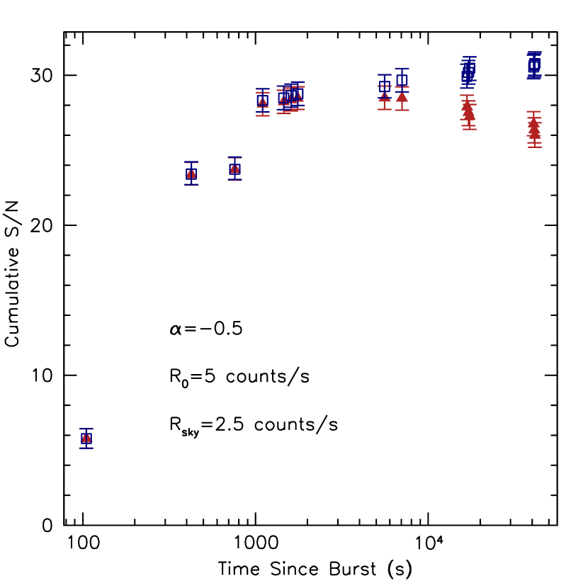
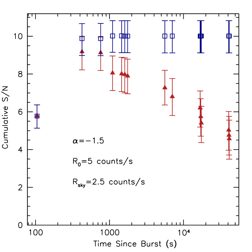
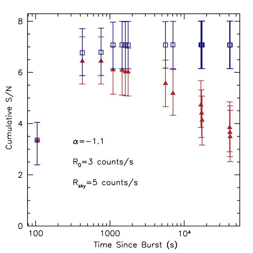
Optical temporal decay slopes for GRB afterglows are usually observed to be in the range $\alpha=-0.5$ to $-2.0$, with an average of about $-0.9$ (Oates et al., 2008). To see how the effectiveness of optimal coaddition is affected by different decay slopes, data were coadded for simulated lightcurves with a range of decay slopes, while the other parameters were held constant. Figure 1 shows the cumulative $S/N$ after coadding the data through each observing interval, using both unweighted, and optimally weighted coaddition, for two different values of the decay slope. Error bars show the $68.3\%$ (nominal $1\sigma$) confidence limits from the results of 1000 simulations. In each case, the unweighted $S/N$ reaches a peak value, then decreases as more data are coadded. This happens because the noise dominates the observations to a greater extent with each successive observation. In contrast, the $S/N$ of the optimally weighted data rises, then flattens to a nearly constant value at long post-burst times. The late-time data contributes very little signal or noise, so the $S/N$ values remain almost unchanged. The effect is the same, regardless of the value of the decay slope, but the relative difference between the final weighted and unweighted $S/N$ is greatest for the data with the steepest decay slope. When the lightcurves are steep, the afterglow fades below the noise level more quickly, so the unweighted $S/N$ drops more rapidly, while the optimally weighted $S/N$ flattens out sooner.

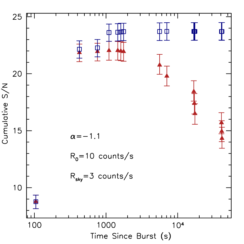
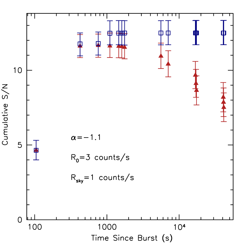
Figure 2 shows how the coadded $S/N$ is affected by differences in the initial count rate; the decay slope and background count rates were fixed at typical values. The results show that the final weighted $S/N$ is significantly better than the unweighted $S/N$ in all cases, and that optimal coaddition has the greatest potential to improve the final $S/N$ when the count rate is low. These statements are true in a statistical sense, but at low count rate, there is no guarantee that the cumulative weighted $S/N$ at any observing time will exceed the unweighted value, as the dispersion of the simulations shows. Nonetheless, as shown by Fig. 2, in typical cases optimal coaddition is more likely to result in a significant ($S/N>3$) detection, than when using unweighted coaddition.

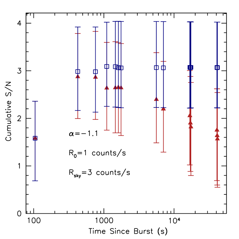
The background count rate clearly affects the detectability of fading afterglows. The background in UVOT images (although low compared to ground-based telescope images) can change greatly from filter to filter, and even among images using the same filter, depending on the directions of the Sun, Earth, and Moon. Figure 3 shows that optimal coaddition improves the $S/N$ in the presence of a wide range of background rates (with decay slope and initial count rate fixed in the simulations), particularly when the background rate is high. When background count rates are very low, as is often the case with X-ray telescopes, there is little benefit from optimal coaddition. For most optical and infra-red detectors, the background is usually the dominant noise factor, so optimal coaddition is worth the minimal implementation effort.

Often the decay slope is unknown, or is not known with great accuracy, so it is of interest to know how the final $S/N$ depends upon the decay slope used in the optimal coaddition. Simulations were made using typical values of the true decay slope $\alpha=-1.2$, the initial afterglow count rate $R_{1}=3\,{\rm counts\,s^{-1}}$, and the background count rate $C_{sky}=2.5\,{\rm counts\,s^{-1}}$. The model decay slope $\alpha_{model}$ (not necessarily the same as the true slope), used for the optimal coaddition was varied over a wide range of values. The median final $S/N$ in the coadded data simulations were calculated for each value of $\alpha_{model}$. The results are shown in Fig. 4. As expected, the final $S/N$ is maximized when the model decay slope closely matches the true slope. Figure 4 shows that, at least for typical cases, there is some leeway in the value of the model decay slope; differences of up to a few tenths in the slope change the final $S/N$ only a small amount. However, the model slope value cannot be arbitrarily different from the true value, or the final $S/N$ can actually drop well below the maximum $S/N$ in the unweighted case (shown by a dashed line in Fig. 4).

The results shown in Fig. 4 suggest a way to estimate the decay slope when it is not known. Optimal data coaddition can be repeated for a data set, for a range of values of the model decay slope. The value that maximizes the final $S/N$ is most likely to come closest to the true decay slope. For the example given here, we calculated the value of the decay slope that maximized the $S/N$ in the optimally coadded data, for each simulated light curve. The mean value of the decay slope was $\alpha=-1.20$ with a standard deviation among the simulations of $\sigma(\alpha)=0.19$. The decay slope estimation technique works well even in cases for which an afterglow is detected only after optimal coaddition. For example, in simulations where the afterglow decay slope is $\alpha=-0.9$ (the average given by Oates et al. (2008)), the initial count rate is $R_{1}=0.9\,{\rm counts\,s^{-1}}$, and the background count rate $C_{sky}=5.0\,{\rm counts\,s^{-1}}$, the optimally coadded $S/N$ is just over 3, while the estimated value of the decay slope is $\alpha=-0.89\pm 0.44$. Thus, this technique can be used to calculate reasonable estimates of the decay slope, even in low $S/N$ circumstances.

As mentioned earlier, X-ray and optical lightcurves usually do not track each other very well, particularly at early times. There are exceptions to this (e.g. Blustin et al., 2006; Grupe et al., 2007), but usually the X-ray decay slope is steeper than the optical slope (Oates et al., 2008), so at best the X-ray slope can be used as a lower limit for the optical slope estimate. When the optical slope is unknown, the best approach for optimal coaddition is probably to assume a range of reasonable decay slopes, bracketed at the steep end by the X-ray slope, and to calculate limiting magnitudes in each case.

5. Application to Swift GRB Image Data

5.1. Optically Bright Bursts

To demonstrate the effect of optimal coaddition on real data, imaging data from the bright well-sampled optical afterglow of GRB 050525A were coadded using the weighted and unweighted methods. The GRB was discovered by the Swift BAT, and the spacecraft slewed to the source immediately (Band et al., 2005). The UVOT began observations about 65s after the burst, and a bright afterglow was detected in images taken with all seven UVOT filters (Holland et al., 2005). UVOT imaging data of the afterglow field were collected up to about $1.2\times 10^{6}$s after the burst; we have used data only up to a few $\times 10^{5}$s after the burst, since the much later time data are entirely consistent with no source flux and add nothing to this example. Full analysis of the Swift data was presented by Blustin et al. (2006). Here we show how the $S/N$ of UVOT data from a well-detected afterglow can depend strongly on how the data are coadded.

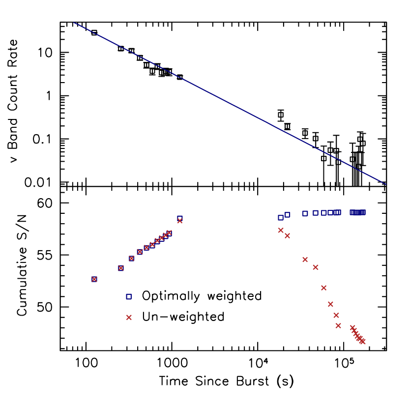
The UVOT $v$ band lightcurve of GRB 050525A is shown in the top panel of Fig. 5, and was constructed as follows. Source plus background counts in the individual $v$ band images were measured using a 3 arcsecond radius aperture. A large background annulus region, centered on the afterglow position, and excluding small regions around any detected stars near the annulus, was used to estimate the background counts. Source counts were measured by subtracting the expected average background counts inside the source extraction region from the total counts inside that region. A power law model was fit to the lightcurve by finding the parameters that minimized the $\chi^{2}$ value of the fit, using the linear count rate data and the associated uncertainties. The best fit power law has an index $\alpha=-1.03$, and is shown in Fig. 5. The value for the power law index is fairly close to that found by Blustin et al. (2006), who found a value of $\alpha=-1.14$ when a simultaneous fit was made to data in multiple bands. However, Blustin et al. (2006) found that a single power law does not give a full statistical description of the optical/UV lightcurve in any band. For this example, we have ignored the deviations from a single power law, since they would unnecessarily complicate the analysis, and would provide very little improvement to the optimal coaddition of the data.

The $v$ band data were coadded without weighting, and using optimal weighting according to equation (24). The GRB afterglow counts expected in each image were calculated according to equation (12), using the best fit value of the decay index in the $v$ band. The cumulative $S/N$ at each exposure was calculated from equation (15) for the unweighted data, and from equation (25) for the weighted data. The bottom panel of Fig. 5 shows the cumulative $S/N$ for both the weighted and unweighted cases. The $S/N$ values in both cases match each other very closely through the first $\approx 1000$s after the burst. Within that time range, the afterglow was still quite bright, and the noise in the images is dominated by the counts from the afterglow itself; optimal coaddition holds little advantage in that case. However, at later times, when the afterglow count rate had dropped to relatively low values, continued unweighted coaddition of the data becomes detrimental. When all of the data are coadded without weighting, the final $S/N$ is well below that of the first image by itself. When the data are optimally coadded, the $S/N$ at later times actually increases slightly, and levels off at a maximum value.

While coaddition of data in the case of GRB 050525A was not necessary for a detection, this example illustrates the danger of coadding image data without considering the rapidly decaying nature of afterglow lightcurves. At best, unweighted coaddition makes no improvements, and at worst it can severely reduce the quality of coadded data. Optimal coaddition nearly guarantees that the highest $S/N$ will be returned from coadded data, regardless of how many images are coadded. In the next two sections, we illustrate the benefits of optimal coaddition applied to data with low $S/N$ in individual images.

5.2. Optical Detections from Optimally Coadded Data

A considerable fraction of optical GRB afterglows are not significantly detected (at $>3\sigma$) in individual UVOT images taken with a specific filter, but may be significantly detected in the coadded data. An example in which the UVOT $v$ band data reveal no afterglow in individual images, but optimal coaddition results in a detection is GRB 060604. This GRB was discovered by the Swift BAT, and the spacecraft slewed to the source position about 100s after the detection (Page, 2006). An afterglow candidate was found in the initial UVOT white filter image, and later confirmed in unweighted coadded UVOT b and u images (Blustin & Page, 2006), and by ground-based R band images (Tanvir, Rol, & Hewett, 2006). No significant afterglow was found in any of the individual UVOT v band images; unweighted coaddition of over 1100s of data yielded a possible source with a significance of 2.4 $\sigma$ (Blustin & Page, 2006). This case is a good test of the optimal coaddition technique, since we know that there was an optical afterglow in several bands, but that the source was only marginally detected in another band. The optimal coaddition technique was applied to the v band data to determine if the significance of the afterglow could be improved.

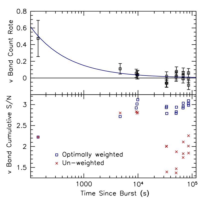
The v band data consist of 17 images, excluding the initial very short settling image (taken while the spacecraft is still slewing), starting about 220 s after the burst, and ending about $10^{5}$ s after the burst. The optimal weights used in equation (19) were determined from measurements of the source counts and background counts in each image, and the temporal decay slope. Source plus background counts in the v band images were measured inside an aperture centered on the known GRB afterglow position, with an aperture of radius 3 arcseconds, which is about optimal for maximizing the $S/N$ of faint sources in UVOT images (Poole et al., 2008; Li et al., 2006a). A large background extraction region was selected to be near the afterglow position, but located so that it did not contain any obviously detected stars. Source counts were determined by subtracting the expected average background counts inside the source extraction region from the total counts inside that region. The v band count rates are shown as a function of time since burst in the top panel of Fig. 6. The best fitting power law was determined using the technique described at the end of § 4. The uncertainty on the power law slope was estimated by calculating the rms of the best slope values in 100 simulated data sets. In each of the simulations the counts in the source and background regions were randomly varied according to a Poisson distribution, with means equal to the measured values. The best power law slope and its uncertainty are $\alpha=-0.62\pm 0.19$; the best fitting power law is shown in Fig. 6. The best slope value is consistent with the value found from the UVOT $white$ band data of $\alpha=-0.62\pm 0.32$ (Blustin & Page, 2006), and from the ground-based $R$ band data of $\alpha=-0.35\pm 0.36$ (Tanvir, Rol, & Hewett, 2006; Garnavich, 2006). It is clear that although none of the individual measurements give a significant detection, the power law decay function fit to all of the data is quite reasonable. In this case, we have used the fitted value of $\alpha$ because it is consistent with the decay slopes in other bands for which there are afterglow detections, and by design it will give the maximum weighted $S/N$. In the absence of a reliable fit in the $v$ band, it would have been appropriate to adopt a value of $\alpha$ given by the results in the other bands.

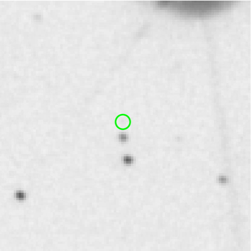
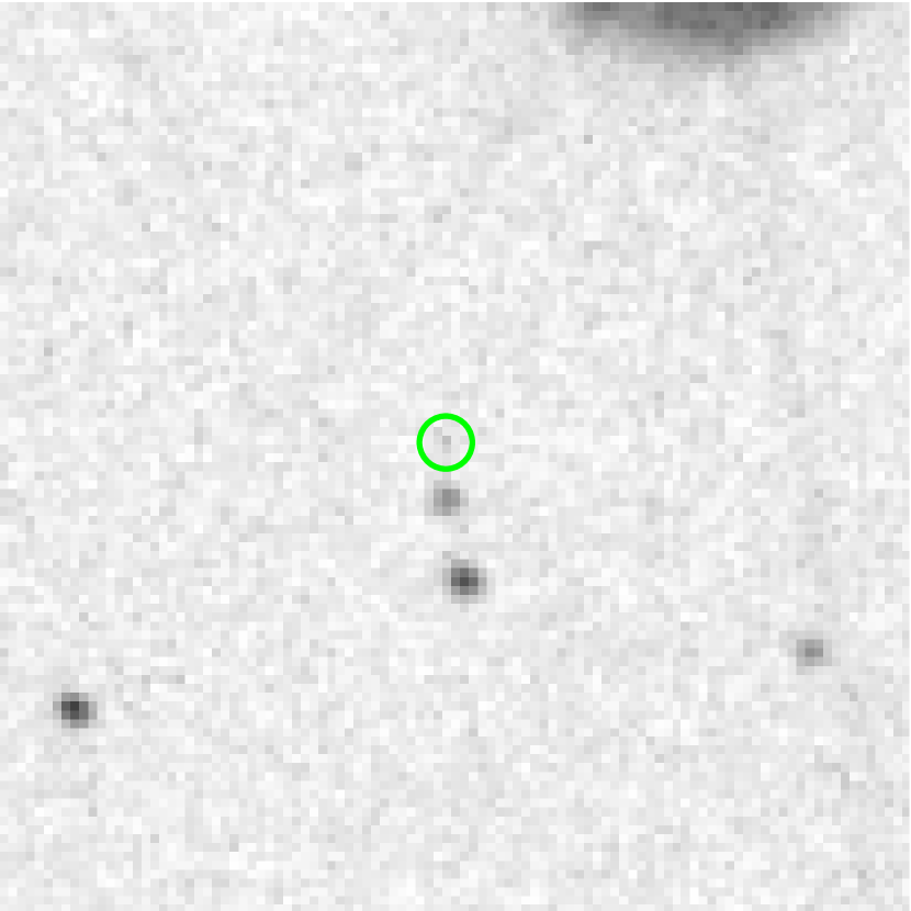
The cumulative $S/N$ at each exposure was calculated from equation (4) for the unweighted data, and from equation (25) for the weighted data. The bottom panel of Fig. 6 shows the cumulative $S/N$ for both the weighted and unweighted cases. The $S/N$ rises with coaddition in both cases up to the first few images. In the unweighted case the $S/N$ drops from a high of about 2.8 to about 2.0 after coadding all of the data. In the optimal weighting case, the $S/N$ rises to about 3.0, and remains quite steady thereafter. Both the maximum unweighted $S/N$ and the final weighted $S/N$ are greater than the value (2.4) reported by Blustin & Page (2006). Using optimal coaddition, the v band data by itself would have been sufficient to detect the optical afterglow. The individual images were coadded using no weighting, and using the optimal weights calculated as described here. Images centered on the afterglow position are shown for both cases in Fig.7. The images have been scaled so that the field stars appear to have the same brightnesses in both images; this allows a direct comparison of the relative coadded brightness of the afterglow in both images. The effect of optimal coaddition is to increase the $S/N$ of the afterglow relative to unweighted coaddition. The process also degrades the $S/N$ of other objects in the image, since for them the weights are not optimal. The afterglow is difficult to see in the unweighted coadded image, but easily seen in the weighted coadded image.

This case illustrates the potential of optimal coaddition to improve the detection rates of GRB afterglows. We plan to apply this method to the entire UVOT GRB database (Roming et al., 2008), to determine if new detections of other afterglows can be achieved.

5.3. Improved Detection Limits for Optical Non-Detections

Optical afterglows have not been detected for many GRBs to date, including GRBs discovered by Swift (Roming et al., 2006). It is important for detection limits to be as deep as possible in order to help understand the “dark burst” phenomenon. Also, when attempting to identify very high redshift burst candidates, fainter detection limits in bluer bands place tighter constraints on the range of possible redshifts. Here we examine the case of GRB 060923A, which is a potentially very high redshift burst, with detections in the $K$ band, but no detections at optical bands, including the UVOT $v$ band.

GRB 060923A was discovered by the Swift BAT, and the UVOT began observations of the burst location about 85 seconds after the trigger (Stamatikos et al., 2006). No afterglow was detected in any of the UVOT images, either singly or coadded, and no afterglow was reported from other observations in the $V$, $R$, $I$, and $J$ bands (Li et al., 2006b; Melandri & Gomboc, 2006; Williams & Milne, 2006; Fox, Rau, & Ofek, 2006). An afterglow was found and confirmed only in the $K$ band (Tanvir, Rol, & Hewett, 2006; Fox, Rau, & Ofek, 2006; Fox, 2006), suggesting that GRB 060923A could be at a very high ($z>10$) redshift or heavily reddened. Subsequent very deep $R$ band observations revealed a possible host galaxy with $R\sim 25.5$ (Tanvir, Rol, & Hewett, 2006), which would favor the reddening hypothesis. Tighter constraints on the bluer band magnitudes would provide correspondingly tighter constraints on either the redshift, or extinction of the GRB.

As discussed in § 3.3, optimal coaddition can be used to find the maximum count rate (and therefore deepest magnitude) that an afterglow could have had in the first image (where the count rate would have presumably been the greatest) without being detected at a given significance level. The detection limit calculations require the exposure start and stop times, an estimate of the afterglow decay rate, and a measurement of the background counts at the GRB position in each image. UVOT images of the burst position were taken in the $v$ band from about 85 s to about 11 ks after the trigger. Background counts in each of the images were estimated for a three arcsecond radius aperture at the reported location of the $K$ band afterglow. The temporal decay rate is unknown, but reasonable estimates can be made from several arguments. First, the $K$ magnitude of the afterglow dropped by at least 0.9 magnitudes from about 6.7 ks to 86 ks after the burst, which means the $K$ band decay slope was less than $\alpha_{K}=-0.33$. Second, the XRT lightcurve faded at two distinct rates: $\alpha_{XRT1}=-2.7$ from about 80 to 400 s, and $\alpha_{XRT2}=-1.23$ after about 4000 s (Conciatore, 2006). These values bracket typical optical afterglow decay slopes; calculations were made using all three values.

Detection limits for a $S/N$ of three in the first UVOT $v$ band image were made for the image by itself, the unweighted coadded image, and the optimally weighted coadded image, as described in § 3.3. The count rate limits were converted to standard UVOT $v$ band magnitudes using the zero points and aperture corrections given by Poole et al. (2008). The results for each of the three decay slopes are given in Table 1. The single image limit is $v=20.22$. For unweighted coaddition, there is little ($v=20.26$) or no improvement with a shallow decay slope ($\alpha=-0.33$), and the limit actually becomes worse with steep decay slopes. The reason for this is that noise in the later images degrades the $S/N$ of unweighted coadded images, so that a brighter source in the first image is required to produce a significant detection in the final coadded image. For a shallow slope, the optimally weighted $v$ band limit ($v=20.42$) in the first frame is significantly deeper than the single frame and unweighted coaddition limits. For steep decay slopes, the optimally weighted limit is virtually the same as the single frame limit (and much better than the unweighted coaddition limit). There is little improvement over the single frame limit in this case, because the steep lightcurve decay makes the later image weights very small, so that they contribute very little to the final $S/N$.

The early UVOT $v$ band detection limits are the deepest reported for GRB 060923A. Any estimate of either a photometric redshift, or an extinction value for this burst, must be consistent with the detection limits. The reported $K$ band detection measurement was made more than $6200$ s after the first $v$ band measurement. Given the range of decay slopes considered, the $v$ band magnitude limit at the time of the $K$ band measurement would be at least 1.3 magnitudes fainter than in the first image. This would place even tighter constraints on either the redshift or extinction. The same analysis can be applied to time series images of any non-detected GRB afterglow to improve the detection limits.

6. Discussion and Summary

Image addition for the detection of variable objects, or the improvement of $S/N$, can benefit significantly from proper weighting. Data from rapidly varying sources, such as GRB afterglows, stands to benefit the most from optimal coaddition. In fact, it can be counterproductive not to optimally weight the data when coadding. We have shown how optimal coaddition can ensure the best $S/N$ for rapidly varying GRB afterglow data, even to the point of recovering previously undetected sources, and can place tighter detection limits on image data sets.

We have assumed a simple power law model for the optical lightcurve; this will clearly be inadequate in many cases (Oates et al., 2008). A spectral extrapolation from the X-ray to the optical lightcurve may provide a reasonable estimate at early times before the forward shock peak. The spectral index $\beta$ should vary between $\beta=(p-1)/2$ and $\beta=p/2$ where $p$ is the electron index (Sari et al., 1998). Given a range of possible $p$ values, one could predict a range of possible optical lightcurves. However, at early times in many X-ray lightcurves, there is a fast decay phase with superimposed flaring activity, which rarely has a counterpart at optical wavelengths. It is probably better in almost all cases to assume an average optical lightcurve (e.g. Oates et al., 2008) rather than extrapolate from an X-ray lightcurve. In any case, it is straightforward to adapt the coaddition technique to arbitrary lightcurves.

The technique can also be applied to observations of any variable source (e.g. supernovae, active galactic nuclei, cataclysmic variable stars), as long as a reasonable estimate of the lightcurve is available. Optimal coaddition is most beneficial when count rates are low, background is high, and the rate of source variability is high. All of these factors often apply to optical observations of GRB afterglows. Optical observations have been used in the examples presented here, but the technique is equally applicable to UV, infra-red, and X-ray imaging data that has Poisson noise characteristics. The benefit to X-ray and possibly UV data may not be as great as for other frequency ranges, since the background count rates are often quite low. However, there would likely be some improvement in $S/N$ or detection limits, and no loss in either, when the source count rates are comparable to the background rates.

There are other ways of improving $S/N$ that could probably be used in combination with the optimal coaddition technique described here. For example, we have used simple circular apertures to extract source counts in individual images; if the image point spread function can be determined with precision, there is the potential for optimally extracting the counts in each image, or the final coadded image. A related optimal pixel weighting technique has been described by Naylor (1998). In addition, if the characteristics (aside from source brightness) of images differ significantly from frame to frame (which is usually not the case for UVOT data), there are techniques to optimally coadd the images to achieve improved $S/N$ or image resolution (Fischer & Kochanski, 1994). As another example, the UVOT can observe in event mode, by tagging the arrival time of individual detected photons. This allows the possibility of optimally weighting individual events, rather than integrated images, which could improve the $S/N$ of afterglow data, particularly at early post-burst times. We also caution that the equations derived here assume count rates high enough that Gaussian noise statistics can be assumed, but at extremely low count rates that assumption may not apply, and other approaches should be considered.

We will apply optimal image coaddition to all of the GRB afterglow data obtained with the Swift UVOT. The primary goal will be the recovery of previously undetected afterglows, but at a minimum, the detection limits will be improved, placing stronger constraints on the existence of so-called dark GRBs.

Table 1GRB 060923A UVOT $v$ band magnitude limits for the first image.

$\alpha$	Single	Unweighted	Optimal
	Image	Coaddition	Coaddition
-0.33	20.22	20.26	20.42
-1.23	20.22	19.60	20.22
-2.70	20.22	19.53	20.22

Figure 1.— Cumulative $S/N$ as a function of time since the burst, for coadded simulated GRB afterglow data, with a shallow decay slope (left) and a steep decay slope (right). The temporal decay slopes $\alpha$, and the initial count rate $R_{1}$, of the lightcurve models are given, along with the background count rate $R_{sky}$. Each point corresponds to an observation in a relatively short time interval. Unweighted coadded data is shown by red triangles; optimally weighted coadded data is shown by blue squares. The error bars span the $68.3\%$ confidence limits in the results of 1000 simulations.

Figure 2.— Cumulative $S/N$ as a function of time since the burst, for coadded simulated GRB afterglow data, with a relatively low initial count rate (left) and high initial count rate (right). The temporal decay slope $\alpha$, and the initial count rates $R_{1}$, of the lightcurve models are given, along with the background count rate $R_{sky}$. Each point corresponds to an observation in a relatively short time interval. Unweighted coadded data is shown by red triangles; optimally weighted coadded data is shown by blue squares. The error bars span the $68.3\%$ confidence limits in the results of 1000 simulations.

Figure 3.— Cumulative $S/N$ as a function of time since the burst, for coadded simulated GRB afterglow data, with a high background count rate (left) and a low background count rate (right). The temporal decay slope $\alpha$, and the initial count rate $R_{1}$, of the lightcurve models are given, along with the background count rates $R_{sky}$. Each point corresponds to an observation in a relatively short time interval. Unweighted coadded data is shown by red triangles; optimally weighted coadded data is shown by blue squares. The error bars span the $68.3\%$ confidence limits in the results of 1000 simulations.

Figure 4.— Final $S/N$ in the optimally coadded data as a function of the model temporal decay index $\alpha_{model}$, for simulated GRB afterglow data. The true decay index is $-1.2$, and the simulations used an initial count rate of 3 ${\rm cts\,s^{-1}}$, and a background count rate of 2.5 ${\rm cts\,s^{-1}}$. The points give the median values from 1000 simulations, and the error bars show the uncertainty on the median value (not the dispersion in the simulations). The dashed line shows the maximum $S/N$ from unweighted coadded data averaged over the simulations.

Figure 5.— Lightcurve (top), and cumulative $S/N$ (bottom) for UVOT $v$ band image data of GRB 050525A, as a function of time since the burst. Error bars on the lightcurve represent count rate uncertainties for measurements using individual images. In the $S/N$ plot, red x’s show the results of unweighted coaddition; blue squares show the results of optimal weighting coaddition.

Figure 6.— Light curve (top), and cumulative $S/N$ (bottom) for UVOT $v$ band image data of GRB 060604, as a function of time since the burst. Error bars on the lightcurve represent count rate uncertainties for measurements using individual images. In the $S/N$ plot, red x’s show the results of unweighted coaddition; blue squares show the results of optimal weighting coaddition.

Figure 7.— Coadded UVOT $v$ band images of GRB 060604. Left — result from unweighted coaddition. Right — result from optimally weighted coaddition. Each image is $4\times 4$ arcmin on a side. The images have been scaled so that the brightnesses of the field stars appear nearly the same in both images. The reported location of the afterglow, detected in other bands, is at the center in each case. The circles show the 3 arcsec radius apertures used to extract the source counts. In the unweighted case, the $S/N$ of the counts in the source region is about 2.0, while in the weighted case it is about 3.0.

References

- Akerlof et al. (1999) Akerlof, C., et al. 1999, Nature, 398, 400
- Band et al. (2005) Band, D., et al. 2005, GCN Circ. 3466, http://gcn.gsfc.nasa.gov/gcn3/3475.gcn3
- Barthelmy et al. (2005) Barthelmy, S. D., et al. 2005, Space Science Reviews, 120, 143
- Barthelmy et al. (1998) Barthelmy, S. D., Butterworth, P. S., Cline, T. C., & Gehrels, N. 1998, in AIP Conf. Proc. 428, Gamma-Ray Bursts: 4th Huntsville Symposium, eds. C. A. Meegan, R. D. Preece, & T. M. Koshut (New York: AIP), 99
- Barthelmy et al. (1995) Barthelmy, S. D., Butterworth, P., Cline, T. L., Gehrels, N., Fishman, G. J., Kouveliotou, C., & Meegan, C. A. 1995, Ap&SS, 231, 235
- Blustin et al. (2006) Blustin, A. J., et al. 2006, ApJ, 637, 901
- Blustin & Page (2006) Blustin, A. J., Page, M. J., 2006, GCN Circ. 5219, http://gcn.gsfc.nasa.gov/gcn3/5219.gcn3
- Burrows et al. (2005) Burrows, D. N., et al. 2005, Space Science Reviews, 120, 165
- Campana et al. (2006) Campana, S., et al. 2006, Nature, 440, 164
- Conciatore (2006) Conciatore, M. L., 2006, GCN Circ. 5599, http://gcn.gsfc.nasa.gov/gcn3/5599.gcn3
- Dai et al. (2007) Dai, X., Halpern, J. P., Morgan, N. D., Armstrong, E., Mirabal, N., Haislip, J. B., Reichart, D. E., & Stanek, K. Z. 2007, ApJ, 658, 509
- Fischer & Kochanski (1994) Fischer, P., & Kochanski, G. P. 1994, AJ, 107, 802
- Fox, Rau, & Ofek (2006) Fox, D. B., Rau, A., & Ofek, E. O. 2006, GCN Circ. 5597, http://gcn.gsfc.nasa.gov/gcn3/5597.gcn3
- Fox (2006) Fox, D. B. 2006, GCN Circ. 5605, http://gcn.gsfc.nasa.gov/gcn3/5605.gcn3
- Garnavich (2006) Garnavich, P. & Karska, A. 2006, GCN Circ. 5253, http://gcn.gsfc.nasa.gov/gcn3/5253.gcn3
- Gehrels et al. (2004) Gehrels, N., et al. 2004, ApJ, 611, 1005
- Grupe et al. (2007) Grupe, D., et al. 2007, ApJ, 662, 443
- Holland et al. (2002) Holland, S. T., et al. 2002, AJ, 124, 639
- Holland et al. (2005) Holland, S. T., et al. 2005, GCN Circ. 3475, http://gcn.gsfc.nasa.gov/gcn3/3475.gcn3
- Horne (1986) Horne, K. 1986, PASP, 98, 609
- Jakobsson et al. (2004) Jakobsson, P., et al. 2004, New Astronomy, 9, 435
- Li et al. (2006a) Li, W., Jha, S., Filippenko, A. V., Bloom, J. S., Pooley, D., Foley, R. J., & Perley, D. A. 2006, PASP, 118, 37
- Li et al. (2006b) Li, W., Butler, N., Bloom, J. S., & Filippenko, A. V. 2006, GCN Circ. 5584, http://gcn.gsfc.nasa.gov/gcn3/5584.gcn3
- Marshall (2007) Marshall, F. E., 2007, in Proceedings of Gamma Ray Bursts 2007, Santa Fe, NM, 05-09 November
- Mason et al. (2005) Mason, K. O., Blustin, A. J., & Roming, P. W. A. 2005, in Proceedings of the X-ray Universe 2005, San Lorenzo de El Escorial (Spain), 26-30 September (astro-ph/0511322).
- Mason et al. (2004) Mason, K. O., Breeveld, A., Hunsberger, S. D., James, C., Kennedy, T. E., Roming, P. W. A., & Stock, J. 2004, Proc. SPIE, 5165, 277
- Melandri & Gomboc (2006) Melandri, A., & Gomboc, A. 2006 GCN Circ. 5586, http://gcn.gsfc.nasa.gov/gcn3/5586.gcn3
- Mészáros & Rees (1999) Mészáros, P., & Rees, M. J. 1999, MNRAS, 306, L39
- Meszaros & Rees (1997) Meszaros, P., & Rees, M. J. 1997, ApJ, 476, 232
- Morgan et al. (2005) Morgan, A., Grupe, D., Gronwall, C., Racusin, J., Falcone, A., Marshall, F., Chester, M., & Gehrels, N. 2005, GCN Circ., 3577
- Naylor (1998) Naylor, T. 1998, MNRAS, 296, 339
- Nousek et al. (2006) Nousek, J. A., et al. 2006, ApJ, 642, 389
- Oates et al. (2008) Oates, S., et al. 2008, in prep.
- Page (2006) Page, M. J., et al., 2006, GCN Circ. 5212, http://gcn.gsfc.nasa.gov/gcn3/5212.gcn3
- Poole et al. (2008) Poole, T., et al. 2008, MNRAS, 383, 627
- Roming & Mason (2006) Roming, P. W. A., & Mason, K. O. 2006, in AIP Conf. Proc. 836, Gamma-Ray Bursts in the Swift Era, ed. S. S. Holt, N. Gehrels, & J. A. Nousek (Melville: AIP), 224
- Roming et al. (2005a) Roming, P. W. A., et al. 2005a, Space Science Reviews, 120, 95
- Roming et al. (2005b) Roming, P. W. A., et al. 2005b, GCN Circ., 3249
- Roming et al. (2006) Roming, P. W. A., et al. 2006, ApJ, 652, 1416
- Roming et al. (2008) Roming, P. W. A., et al. 2008, in preparation
- Rykoff et al. (2006) Rykoff, E. S., et al. 2006, ApJ, 638, L5
- Rykoff et al. (2004) Rykoff, E. S., et al. 2004, ApJ, 601, 1013
- Sari & Piran (1999) Sari, R., & Piran, T. 1999, ApJ, 517, L109
- Sari et al. (1998) Sari, R., Piran, T., & Narayan, R. 1998, ApJ, 497, L17
- Schady et al. (2005) Schady, P., et al. 2005, GCN Circ., 3057
- Stamatikos et al. (2006) Stamatikos, M., et al. 2006, GCN Circ. 5583, http://gcn.gsfc.nasa.gov/gcn3/5583.gcn3
- Tanvir, Rol, & Hewett (2006) Tanvir, N., Rol, E., & Hewett, P., 2006, GCN Circ. 5216, http://gcn.gsfc.nasa.gov/gcn3/5216.gcn3
- Wei et al. (2006) Wei, D. M., Yan, T., & Fan, Y. Z. 2006, ApJ, 636, L69
- Williams & Milne (2006) Williams, G. G., & Milne, P. A. 2006, GCN Circ. 5588, http://gcn.gsfc.nasa.gov/gcn3/5588.gcn3
- Zhang et al. (2006) Zhang, B., Fan, Y. Z., Dyks, J., Kobayashi, S., Mészáros, P., Burrows, D. N., Nousek, J. A., & Gehrels, N. 2006, ApJ, 642, 354