Evidence of Turbulence-like Universality on the Formation of Galaxy-sized Dark Matter Haloes

Abstract

Context. Although the theoretical understanding of the nonlinear gravitational clustering has greatly advanced in the last decades, in particular by the outstanding improvement on numerical N-body simulations, the physics behind this process is not fully elucidated.

Aims. The main goal of this work is the study of the possibility of a turbulent-like physical process in the formation of structures, galaxies and clusters of galaxies, by the action of gravity alone.

Methods. We use simulation data from the Virgo Consortium, in ten redshift snapshots (from 0 to 10). From this we identify galaxy-sized and cluster-sized dark matter haloes, by using a FoF algorithm and applying a boundedness criteria, and study the gravitational potential energy spectra.

Results. We find that the galaxy-sized haloes energy spectrum follows closely a Kolmogorov’s power law, similar to the behaviour of dynamically turbulent processes in fluids.

Conclusions. This means that the gravitational clustering of dark matter may admit a turbulent-like representation.

1 Introduction

In a general framework, the standard model of structure formation is based on the gravitational Jeans instability criterion (e.g. Linder 1997) which neglects viscous, turbulence and diffusion effects. In this model, the gravity acts to amplify the tiny random fluctuations in the primordial density field to the significantly overdense structures we see today (galaxies, groups, clusters and superclusters). As long as the density contrast of the fluctuations remains small ($\delta\ll$ 1) – in early times for small spatial scales (like the ones of galaxies) and until the present time for the largest scale structures – the amplitude of these fluctuations grows linearly. In this regime all scales evolve independently (e.g. Sahni & Coles 1995), and the random-phase nature of the initial density field is preserved. Analytically, the equations of motion of the particles that compose the “cosmic fluid” can be successfully solved by means of the perturbation theory. It turns out that, in the hierarchical scenario, fluctuations of increasing spatial scale successively enter a nonlinear regime, collapse and evolve to the virial equilibrium. Conversely to the case of the linear regime, there is no general exact analytic solution for the evolution of structures on this stage (e.g. Padmanabhan 2006).

The search for a theoretical understanding of the nonlinear gravitational clustering has greatly advanced in two distinct directions: by constructing analytical approximation schemes and by evolving numerical N-body simulations. While the attempts on the first approach are limited to the domains of validity of the approximations, the ones on the last reproduce quite well most of the observed properties of the actual structures (see, for instance, Springel et al. 2005), but do not clarify completely our understanding of the physics behind it.

On the analytical front, the most appealing proposals have been the ones based on a hydrodynamical approach. The original and simplest model of this type is the one called Zel’dovich Approximation (ZA, Zel’dovich 1970), which considers that the velocity of the fluid elements can be expressed at any time in terms of the initial gravitational potential, that is, they move in the field without modifying it. Remarkably this model predicts the walls (pancakes), filaments, clumps and voids that characterize the large scale structure. Nevertheless, the lack of self-gravity leads to the dissolution of the structures after the first crossing of the particles. Further progress was achieved with a series of approximations referred to as adhesion models (Gurbatov et al. 1989; Shandarin & Zel’dovich 1989; Ribeiro & de Faria 2005). Mathematically, these models are based on the three-dimensional Burgers’ equation (Burgers 1940) which introduces an ad hoc artificial viscosity that slows down the particles as they approach the pancakes and filaments. The alternative schemes are mostly extensions of the ZA, among which are the more recently proposed Lagrangian approximations (see, e.g., Sahni & Coles 1995; Makler et al. 2001; Bernardeau et al. 2002, and references therein).

One possibility that was not much explored is that the formation of structures is more closely related to hydrodynamics, for example, by the existence of a “turbulent-like” behaviour of the dark matter clustering process. The idea comes from the characteristic pattern of the large scale structure that resembles the turbulent pattern of fluids, although collisionless dark matter is the responsible for such pattern (baryonic matter effects take place mostly on smaller scales, while dark energy is expected to be acting more recently).

In this paper we use a N-body simulation from the Virgo Consortium to to look for signatures of a turbulent-like process in the formation of structures. For this sake we detect systems of different scales, from galactic size subhaloes to supercluster size super-haloes, study some of their evolutionary properties, and evaluate the gravitational energy of bound systems.

2 The Virgo N-body Simulation

Our data came from the intermediate scale cosmological N-body simulations run by the Virgo Consortium, which are reported in Jenkins et al. (1998). Below we briefly describe the main steps and characteristics of these simulations (for an extensive review see, for instance, Bertschinger 1998, and references therein).

As usual, the fundamental properties of the N-body simulations of structure formation in the Universe are defined by the background cosmological model and the initial perturbations imposed on this background. Four versions of the cold dark matter model are available from the Virgo Consortium project, from which we chose the $\Lambda$CDM one, with cosmological parameters ($\Omega_{M}$, $\Omega_{\Lambda}$, $h$, $\sigma_{8}$) = (0.3, 0.7, 0.7, 0.9). Among the additional (numerical) parameters that characterize the simulation are the simulation box of side 239.5 $h^{-1}$ Mpc and the number of particles, 256³, with individual masses of $6.86\times 10^{10}\,h^{-1}\,M_{\sun}$. Comoving spatial coordinates and periodic boundary conditions were also used (see Jenkins et al. 1998, for details). Ten snapshots are available, at redshifts: 10.0, 5.0, 3.0, 2.0, 1.5, 1.0, 0.5, 0.3, 0.1 and 0.0.

The initial conditions are set by assigning a position and velocity to each particle using an algorithm imposing perturbations on an initially uniform state represented by a “glass” distribution of particles (see, e.g., White 1996). A convenient and efficient method (Efstathiou et al. 1985) for converting the early density fluctuations into these perturbations can be derived from the Zel’dovich (1970) solution:

$$\@vec{x}=\@vec{r}/{\mathit{a}}=\@vec{q}+D\ \@vec{p}\\ \@vec{v}=\frac{d\@vec{r}}{dt}-H\@vec{r}=a\frac{dD}{dt}\@vec{p}$$ (1)

where $\@vec{x}$ is the comoving Eulerian coordinate of a particle, $\@vec{r}$ is its proper Eulerian coordinate, $a(t)$ is the expansion factor (which satisfies the Friedmann equation), $\@vec{q}$ is the Lagrangian coordinate of the particle denoting its initial unperturbed position, $D(t)$ is the growth factor of the linear growing mode, $\@vec{p}(\@vec{q})$ is the displacement field, $\@vec{v}$ is the peculiar velocity of the particle and, finally, $H(t)=d\ln a/dt$, is the Hubble parameter. The first term of the displacement equation describes the cosmological expansion, while the second denotes the perturbation. The initial velocity field is defined by the initial density fluctuations:

$$\nabla.\@vec{p}=-\delta/D$$ (2)

where $\delta(\@vec{x},t)=[\rho-\bar{\rho}]/\bar{\rho}$,  $\rho(\@vec{x},t)$ is the local mass density and $\bar{\rho}(t)$ is the spatial mean density.

Since cosmological N-body simulations are intended to follow the evolution of the dark matter from the linear regime into the deeply nonlinear regime, they must begin with the expected distribution of matter, at some early epoch, produced by the linear evolution of primordial fluctuations. If these fluctuations are Gaussian, they can be fully described by the density fluctuation power spectrum (PS), $P(k,t)=\langle|\delta_{k}(t)|^{2}\rangle$. This PS can be written as the product of an initial power law, produced by the process which generated the fluctuations (typically the amplification of quantum fluctuations during inflation), a transfer function $T(k)$ representing the linear evolution of each mode through the early expansion history (matter domination, baryon-photon decoupling, etc.), and the growth factor $D(t)$ governing the later linear evolution after decoupling:

$$P(k,t)=Ak^{n}T(k)^{2}D(t)^{2}$$ (3)

where $A$ is a normalization factor encoding the overall amplitude of the initial fluctuactions (generally determined from $\sigma_{8}$).

For the Virgo simulations, a Harrison-Zel’dovich $n=1$ spectral index was used, and also the approximation given by Bond & Efstathiou (1984) for the transfer function:

$$T(k)={\{1+[\mathrm{a}q+(\mathrm{b}q)^{3/2}+(\mathrm{c}q)^{2}]^{\nu}\}^{-1/\nu}}$$ (4)

where $q=k/\Gamma$, $\mathrm{a}=6.4\,h^{-1}$ Mpc, $\mathrm{b}=3\,h^{-1}$ Mpc, $\mathrm{c}=1.7\,h^{-1}$ Mpc and $\nu=1.13$. So, the shape of the PS is determined by the parameter $\Gamma=\Omega_{0}h$. The amplitude $A$, on the other hand, was obtained from the observed abundance of galaxy clusters (Jenkins et al. 1998).

Given the initial conditions, that is, the initial position and velocity vector of each particle, the simulation is run in about one thousand timesteps from $z=30$ to $z=0$. Newton’s law and Poisson’s equation, in commoving coordinates, are used to evolve forward in time the particle trajectories:

$$\@vec{x}^{\prime\prime}=-\nabla\phi(\@vec{x}),\\ \phi(\@vec{x})=-G\sum_{j=1}^{N}\frac{m_{j}}{[(\@vec{x}-\@vec{x}_{j})^{2}+\epsilon^{2}]}.$$ (5)

The parameter $\epsilon$ is a softening factor introduced in order to prevent the formation of unphysical binaries and large angle particle scatterings, and to ensure that the two-body relaxation time is sufficiently large to guarantee the collisionless behaviour (Efstathiou & Eastwood 1981). The time integration is performed using a second order leapfrog scheme (Efstathiou et al. 1985). At each timestep the gravitational force of every particle, generated by all others, must be calculated. This is a critically time consuming task if done by direct summation, so that simplifying parallel algorithms may be used to efficiently compute it. The Virgo Consortium used a parallel adaptive P³M algorithm (Couchman, Thomas & Pearce 1995; Pearce & Couchman 1997), which computes long range gravitational forces by smoothing the mass distribution in a mesh (particle-mesh, PM), short range gravitational forces by direct summation (particle-particle, PP), and applying high resolution refinements around strong clustered regions.

3 Identification of dark matter structures

There are many methods for detecting dark matter haloes in N-body simulations. The most simple, used and tested ones are the percolation algorithm (or “Friends-of-Friends”, dubbed FoF, Huchra & Geller 1982; Einasto et al. 1984; Davis et al. 1985) the “Spherical Overdensity” method (Lacey & Cole 1994) and the “DENMAX” sliding scheme (Gelb & Bertschinger 1994).

The FoF algorithm groups together particles that have pair separations smaller than a chosen linking length, $\ell$. This linking length is frequently referred to as $b$ times the mean interparticle separation. The resulting “groups” are bounded by a surface of approximately constant density:

$${{n}\over{\bar{n}}}={{2}\over{(4/3)\pi{\ell}^{3}}}{{1}\over{\bar{n}}}={{3}\over{2\pi{\ell}^{3}}}{\bar{\ell}}^{3}={{3}\over{2\pi}}{{1}\over{b^{3}}}\sim{{1}\over{2b^{3}}}$$ (6)

Assuming that the density profile of these groups can be approximated by isothermal spheres, the average density contrast internal to this surface is given by about 3 times the surface density. The larger is $\ell$ (or $b$), the lower is the density contrast and the higher is the number of particles linked to the groups. In general the value of $b$ is chosen to give a mean overdensity close to the value expected for a virialized object in the framework of the spherical collapse model, $\sim$179. This gives $b=$ 0.2, which seems to be an appropriate value for detecting cluster-sized haloes (Lacey & Cole 1994; Eke et al. 1996; Governato et al. 1999). The main advantages of the FoF method are the simplicity (only one free parameter), the reproduptibility (a unique group catalog for any chosen value of $\ell$) and the capability of detecting haloes of any shape.

The other approach, SO algorithm, identifies density peaks and puts spheres around them, increasing the radius of the spheres until the average density contrast reaches a chosen value. It was proposed to overcome the problem of FoF that may accidently link two distinct lumps if they are connected by a low density bridge of particles. However, it tends to loose the outer portions of ellipsoidal haloes due to the assumption of spherical symmetry (Lacey & Cole 1994).

The DENMAX algorithm, on the other hand, “moves” particles along local density gradients toward density maxima, separating halo candidates by three-dimensional density valleys. The improvement of this method is the application of a self-boundedness check by eliminating particles with positive total energy. Unfortunately, this scheme has the drawback that the results depend on the level of smoothing of the density field (Gelb & Bertschinger 1994).

Nevertheless, the three methods above are found to give similar results (Lacey & Cole 1994; Eke et al. 1996; Audit et al. 1998). The main limitation of these algorithms for detecting structures on N-body simulations appears for small masses (like the ones of galaxies): they do not resolve properly “sub-haloes” embedded in host (cluster-sized) haloes with the usual parameters. Improved versions of FoF, SO and DENMAX – respectively the hierarchical FoF (HFoF, Klypin et al. 1999), the Bound Density Maxima (BDM, Klypin et al. 1999) and the HOP (Eisenstein & Hut 1998) – and also two step algorithms – like the SUBFIND (Springel et al. 2001) and the Physically Self-Bound (Kim & Park 2006) – have been proposed to better identify sub-haloes in crowded regions.

Here we use a different approach. It works, in some sense, like the HFoF algorithm. Since the FoF with $b=$ 0.2 was shown to successfully detect cluster-sized haloes, we use this scheme. A cut in a minimum number of particles is used to eliminate haloes with masses smaller than the ones expected for cluster-sized haloes (see table 1). For galaxy-sized haloes (including sub-haloes) we use FoF with a smaller linking parameter ($b=$ 0.1). This results in a catalog of haloes smaller and denser than the cluster-sized haloes. Also, the equivalent mean density contrast ($\sim$1 300) is close to the one expected for the Milky-Way if one considers the mass estimate of $1.5\times 10^{12}\,h^{-1}\,M_{\sun}$ and the radius of $150\,h^{-1}$ kpc (e.g. Smith et al. 2007; Dehnen et al. 2006; Sakamoto et al. 2003). So, this is appropriate for identifying sub-haloes and also for isolated galaxy-sized haloes. cD galaxies are the most massive galaxies and, since they are transition objects (their halo may be indistinguishable from their parent cluster halo), they are detected as overmassive galaxy-sized haloes. They also coincide with their parent cluster position. For some analyses we excluded these special galaxies by putting a maximum mass limit. We also tentatively identify supercluster-sized haloes by relaxing the linking parameter to $b=$ 1.0 (density contrast about 1.5). Superclusters are not virialized systems, but structures that probably have just detached from the Hubble flow. The volume of the simulation is small for accurate statistics of superclusters, but we can select some typical cases for further analysis (to be published elsewhere).

Table 1: Halo identification and selection parameters ($f$ is the mean density contrast).

Halo size	$b$	$\ell$	$f$	Mass
		(Mpc)		($N_{\mathrm{part}}$)	($M_{\sun}$)
Galaxies	0.1	0.10	1 300	2-150	$>1\times 10^{11}$
Groups/Clusters	0.2	0.18	180	$>$ 100	$>7\times 10^{12}$
Superclusters	1.0	0.92	1.5	$>$ 15 000	$>1\times 10^{15}$

We also applied a boundedness check for galaxy-sized haloes, evaluated in a statistical way. Figure 1 shows the distribution of galaxy-sized halo masses (by the number of grouped particles) with their respective velocity dispersions. From the Virial Theorem we expect that, for relaxed bound structures, these two parameters are correlated, that is, the velocity dispersion is proportional to the square root of the mass. The ridge of points in the lower part of the figure follows closely this relation, as can be seen by the fit (solid line). So, we considered as bound the haloes below the dashed line (about 2.5 rms above the fit). For $z=$ 0.0, 50.7% of the particles remained isolated after the application of the FoF algorithm to search for galaxy-sized haloes, and 10.6% were excluded as unbound haloes. These isolated particles and the particles of excluded haloes are probably associated to galaxies smaller then our detection limit. A similar behaviour was found for the other redshift snapshots.

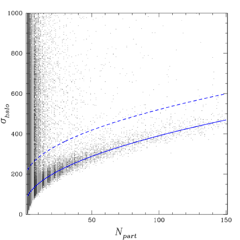
Figure 1: Distribution of galaxy-sized halo masses (N_part) with their respective velocity dispersion ($\sigma_{halo}$), for redshift 0. The solid line is the fit to the points in the main ridge (a power law $\sigma_{halo}\propto{N_{part}}^{1/2}$ is used), while the dashed one represents 2.5 rms of dispersion above this fit.

4 Correlation Functions

In this section we discuss the clustering properties of the galaxy-sized and cluster-sized haloes, found by our percolation scheme, in order to check the consistency of our object catalogs. We measure the two-point (auto)correlation function using the Landy & Szalay (1993) estimator:

$$\xi(r)={{1}\over{RR}}[DD(n_{R}/n_{D})^{2}-2DR(n_{R}/n_{D})+RR]$$ (7)

where $DD$, $DR$ and $RR$ are the pair counts, respectively in the data-data, data-random and random-random catalogs, and $n_{R}$ and $n_{D}$ are the mean number densities in data and random catalogs. We used $n_{R}=n_{D}$ in all cases. We also applied the Davis & Peebles (1983) and Hamilton (1993) estimators to our data and found very similar results on the sampled ranges.

Figure 2 shows the two point correlation functions for the dark matter particles in the simulation (DMCF), for redshifts between 0.0 and 5.0. The results for redshifts 0.0, 0.3, 0.5 and 1.0 are very close to the ones presented by Jenkins et al. (1998) on their third top panel of figure 5, as expected. The $z=$ 0.1 correlation function has a slightly different behaviour on scales larger than 1 $h^{-1}$ Mpc. It is a well established fact that the dark matter (mass) correlation function has a very complex shape and cannot be represented by a single power law in a significant range (e.g. Jenkins et al. 1998; Pearce et al. 1999; Benson et al. 2000; Springel et al. 2005). Another known property that can be clearly seen is that the amplitude of the DMCF evolves considerably with time. Also its slope changes systematically with $z$.

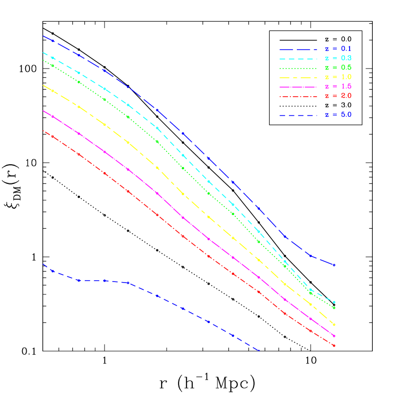
Figure 2: Correlation functions for dark matter particles.

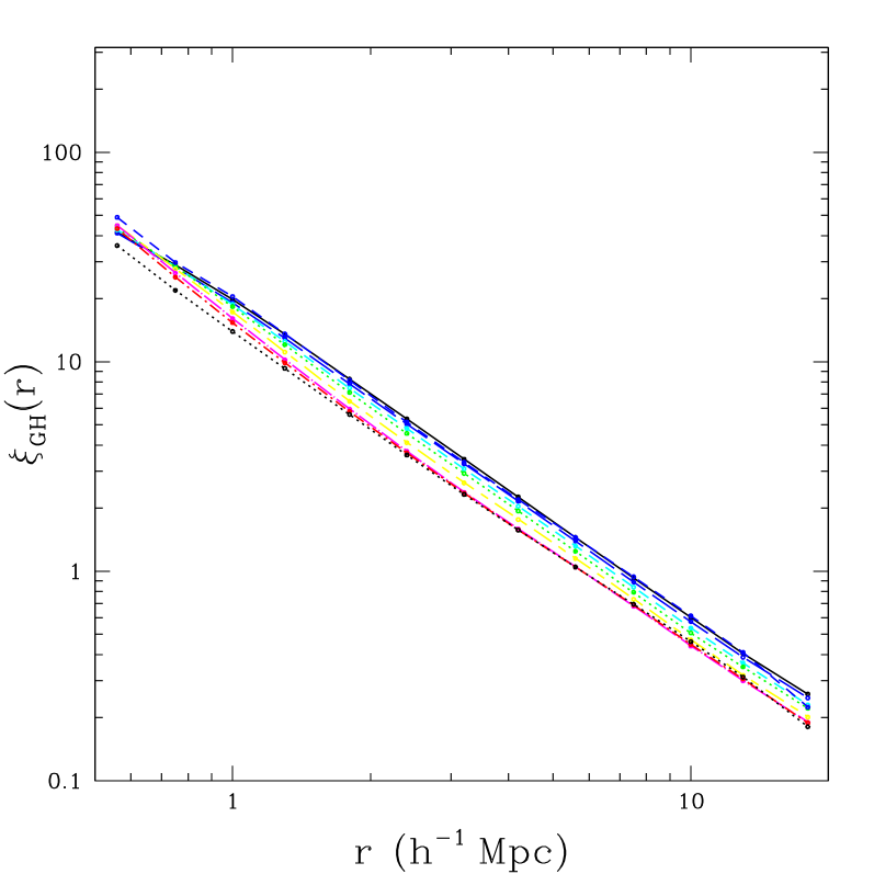
Figure 3: Correlation functions for galaxy-sized haloes. Line types are the same as on Fig. 2.

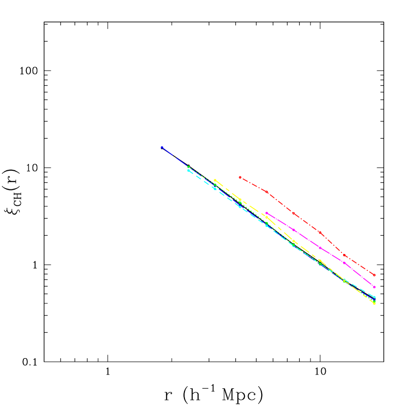
Figure 4: Correlation functions for cluster-sized haloes. Line types are the same as on Fig. 2.

The correlation functions for galaxy-sized haloes (GHCF) are presented on Fig. 3, for the same range of redshifts. Unlike the DMCF, it shows a shape that resembles closely a power law in all redshifts and over a large range of pair separations (here we display the range adequately sampled by our data, $0.5<r<20\,h^{-1}$ Mpc). This behaviour has been pointed as really no more than a coincidence (see, e.g. Springel et al. 2005), but, as we shall see in Sect. 5, this might be related to the emergence of a turbulent-like process in the halo clustering. On small scales (less than a few Mpc) and low redshifts, the GHCF has less power than the DMCF, and the GHCF is said to be “antibiased”. On larger scales, on the other hand, the GHCF function show similar amplitudes to the DMCF for lower redshifts, and so it is “unbiased”. Furthermore, the GHCF evolves very little with redshift (its amplitude grows slightly with time).

Figure 4 displays the correlation functions for cluster-sized haloes (CHCF). One can readily see that, up to redshifts $z\sim 1$, it evolves even slower than the GHCF. At higher redshifts, the CHCF begins to grow. This is a consequence of the correlation between the correlation function of clusters and their masses or richness: at higher redshifts, only the most massive clusters are detected and they are more clustered (Mo & White 1996; Bahcall et al. 2004; Younger et al. 2005).

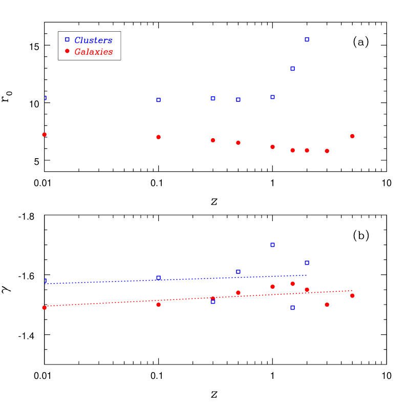
Figure 5: Evolution of the parameters amplitude [panel (a)] and slope [panel (b)] for the power law fit to the correlation functions of galaxy-sized haloes and cluster-sized haloes. The dotted lines are the linear fits to the data.

In order to better characterize the evolution of the correlation strength ($r_{0}$) and slope ($\gamma$) with redshift we fitted power laws to the correlation functions of galaxy-sized and cluster-sized haloes

$$\xi(r)=\left({r\over r_{0}}\right)^{-{\gamma}}$$ (8)

respectively in the ranges 0.6–18 $h^{-1}$ Mpc and 2–18 $h^{-1}$ Mpc. The results can be seen on Fig. 5. Panel (a) shows the evolution of $r_{0}$, which grows slightly with time for both galaxy-sized haloes and cluster-sized haloes (more for the former), except for the high redshift points for which the biased sampling towards more massive objects, as cited above, begins to dominate. Panel (b) displays the $\gamma$ evolution. There is almost no change in the slope, except for probable random noise that also grows with redshift due to the decrease in the number of objects. The mean slope for galaxy-sized haloes and cluster-sized haloes are, respectively, 1.53 and 1.59, with standard deviations of 0.03 and 0.09. This values are smaller than the classical 1.8 slope, but consistent with recent observational results, especially for galaxies (e.g. Padilla & Baugh 2003; Hawkins et al. 2003).

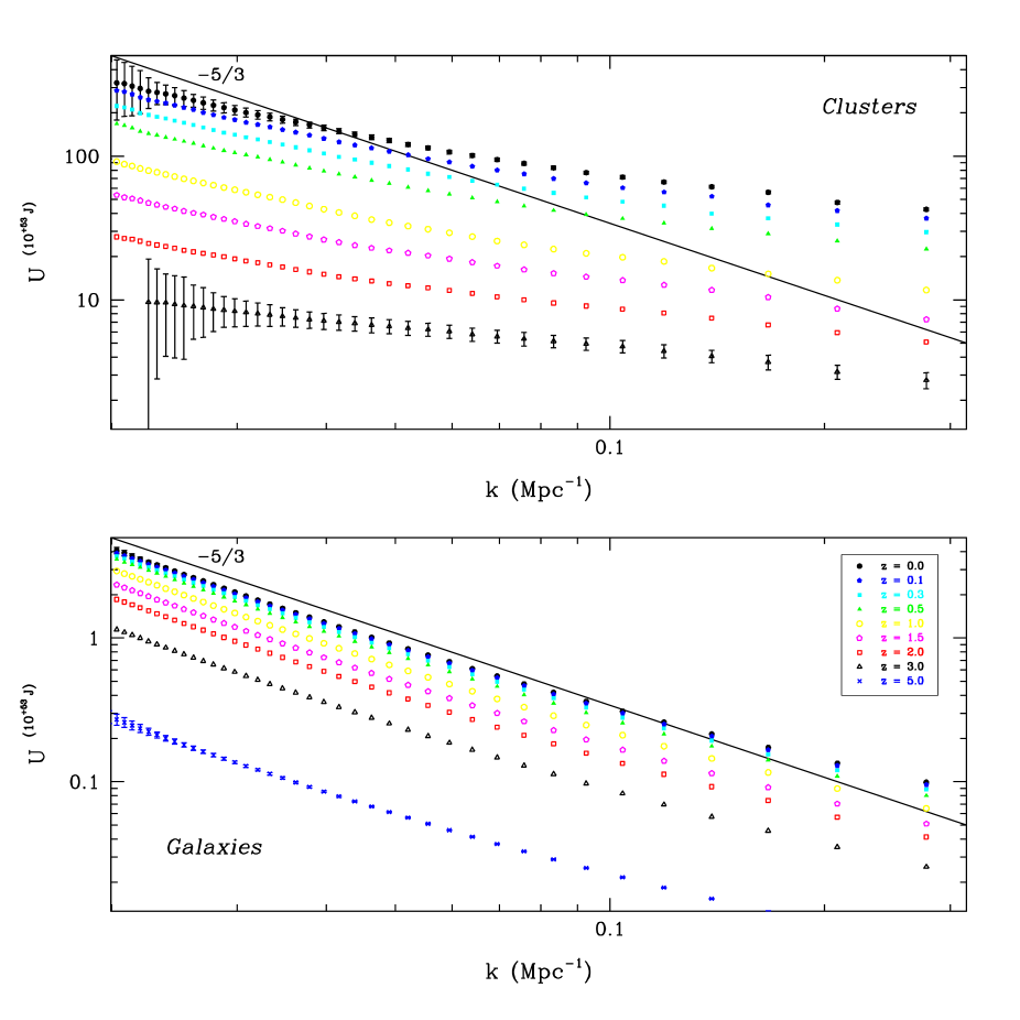
Figure 6: Gravitational energy spectra for cluster-sized haloes (above panel) and galaxy-sized haloes (below panel), for the sampled redshifts. A reference $-5/3$ power law is plotted as a solid line.

5 Turbulence-like Energy Spectra

Now we test the hypothesis of the existence of turbulent-like processes in the formation of structures, searching for their possible signatures. The main characteristic of 3D turbulence is the existence of a kinetic energy cascade. According to this phenomenology, kinetic energy is injected in the fluid at large scales by an external mechanical forcing. Large scale eddies are then deformed and stretched by the fluid dynamics, breaking into smaller eddies. This process is repeated, through a hierarchy of smaller and smaller eddies, until the kinetic energy is finally dissipated into heat by the viscosity of the fluid (Frisch 1995). Within a certain range of intermediate scales, the distribution of energy among turbulence vortices behaves like a power law with exponent $-5/3$. This is the celebrated Kolmogorov’s energy spectrum, and represents the key signature of the “top-down” turbulent cascade scenario. Naturally, in an unbounded medium filled with a collisionless set of particles, the emergence of a turbulent-like behaviour would have a different physical origin than in the standard hydrodynamic turbulence. Nevertheless, the effects of particle trajectory crossings and virialization, as well as the damping effect of the universal expansion, could lead to similar phenomena as observed in standard turbulence. For example, the cosmological dynamics of structure formation could exhibit the power law scaling. This will be the focus of this section. In other words, we will investigate the energy distribution of the cosmic structures discussed above (i.e. galaxies and clusters) to look for the signal of such a turbulent-like behaviour in the form of a power law scaling.

Since we are not dealing with an usual fluid (dark matter is acollisional and, so, not viscous) and we have no energy “injection” in the strict sense, our assumption must be that the energy that produces the turbulent-like behaviour is the gravitational potential energy. Thus, with the lists of identified galaxy-sized and cluster-sized haloes we obtained the energy spectra of the gravitational potential. This was done by estimating, for each halo and in concentric shells, the gravitational energy due to all other haloes:

$$U_{j}={1\over 2}Gm_{j}\sum{m_{i}\over r_{ij}}$$ (9)

where $r_{ij}$ is the distance between the haloes $i$ and $j$. Then we estimate the mean energy (for all haloes) of each shell and build the energy spectra with its cumulative value. The results of this calculation are presented on Fig. 6: panel (a) for cluster-sized haloes and panel (b) for galaxy-sized haloes. The stochastic error estimations (${1}/{\sqrt{N}}$) are plotted only for the first and last redshifts to make the viewing of the figure more clear. The $-5/3$ power law is represented by a solid line. One can easily notice that the energy spectra for the cluster-sized haloes, although following a power law, does not exhibit the Kolmogorov’s index. On the other hand, the one for galaxy-sized haloes follows closely the $k^{-5/3}$ scaling in the wave number range 0.02 to 0.07 (15 to 50 $h^{-1}$ Mpc).

It should be noted that this result differs from the one obtained for highly compressible turbulence in molecular clouds (Kritsuk et al. 2007; Padoan et al. 2007). Three-dimensional simulations of supersonic Euler turbulence show a velocity power spectrum that gets steeper as the Mach number increases, reaching the Burgers slope of $-2$ asymptotically. Kolmogorov’s $-5/3$ scaling is only recovered by mixing the velocity and density statistics, through the computation of density-weighted velocity spectra. The very different context of the present paper (namely, gravitational clustering of large-scale structures, N-body simulation, potential energy spectra) may explain this discrepancy.

To interpret this behaviour we point out that the turbulent-like spectra shown in Fig. 6 have only the inertial regime, without both the typical spectral energy-input and dissipation signatures, which are usually found in standard turbulent systems. As originally suggested by Shandarin & Zel’dovich (1989), a simple turbulent scenario based on the ZA is compatible with a top-down structure formation, where a large structure (pancake), corresponding to the integral scale, forms first then fragments into smaller objects respecting a cascade process. However, the observations and simulations have, for many years, favored a scenario closer to the hierarchical one. In such a way, since the gravitational potential energy is purely attractive, its variation as a function of the “wave number”, defined from the distances among haloes, could be interpreted as a bottom-up cascade process. Physically, because of this attractive nature of gravity, there is always an intermittent intrinsic instability that amplifies any small homogeneity deviation, as does the equivalent hydrodynamic turbulence. Thus, interpreting the results of Fig. 6 as the outcome of a kind of “gravitational turbulence” means that the expansion of the universe in the largest scales is driving an inverse fragmentation process to compensate its deviation from homogeneity in local scales along its evolution. Furthermore, a turbulent-like behaviour may be a typical and essential multi-scaling cosmological feature, requiring, for its robust characterization, the use of appropriate measurement techniques (Ramos et al. 2002; Wuensche et al. 2004; Andrade et al. 2006).

6 Concluding Remarks

We identified galaxy-sized and cluster-sized haloes in an intermediate scale $\Lambda$CDM cosmological N-body simulation by the Virgo Consortium. For these objects we calculated a gravitational potential energy spectra and found that the one for galaxy-sized haloes may be well described by a $-5/3$ power law in the range from 15 to 50 $h^{-1}$ Mpc. It is interesting to note that the same scaling has been found in the observational front, for elliptical galaxies, between potential energy and mass (Márquez et al. 2001). We speculate that this scaling of the energy spectrum, shown in Fig. 6, could be a signature of the Kolmogorov’s universality assumption (Frisch 1995), where the system dynamical structural behaviour is uniquely and universally determined by the scaling and its associated mean energy rate. From our results, the formation of structures in the nonlinear regime seems to be driven by a turbulent-like mechanism, associated with irregular fluctuations in an unstable gravitational field, characterized by combinations of small-scale eddies and larger flow-like structures.

It should be noted that a power-law spectrum by itself does not mean the existence of turbulence. However, the emergence of a (approximately) scale invariant hierarchy of structures as the result of the gravitational clustering process, together with the results of Fig. 6, are consistent with the turbulence-like scenario suggested here. Also, the space-time patterns seen in the simulated data can be interpreted as intermittent nonlinear filaments in a turbulent-like “gravitational” fluid (see, for phenomenological comparison purposes, the turbulent fluid simulated by She et al. 1991). Because of its importance in our approach, it is worth mentioning that there is presently no closed theoretical description of turbulence (e.g. Sreenivasan 1995; Velho et al. 2001; Ramos et al. 2001). Detailed studies, including analyses of higher resolution cosmological simulations and theoretical advances on the models for the nonlinear regime and turbulence itself, are needed to advance on interpreting the apparent turbulent-like behaviour of the structure formation processes presented here.