The Environments of High Redshift QSOs

Abstract

We present a sample of $i_{775}$-dropout candidates identified in five Hubble Advanced Camera for Surveys fields centered on Sloan Digital Sky Survey QSOs at redshift $z\sim 6$. Our fields are as deep as the Great Observatory Origins Deep Survey (GOODS) ACS images which are used as a reference field sample. We find them to be overdense in two fields, underdense in two fields, and as dense as the average density of GOODS in one field. The two excess fields show significantly different color distributions from that of GOODS at the 99% confidence level, strengthening the idea that the excess objects are indeed associated with the QSO. The distribution of $i_{775}$-dropout counts in the five fields is broader than that derived from GOODS at the 80% to 96% confidence level, depending on which selection criteria were adopted to identify $i_{775}$-dropouts; its width cannot be explained by cosmic variance alone. Thus, QSOs seem to affect their environments in complex ways. We suggest the picture where the highest redshift QSOs are located in very massive overdensities and are therefore surrounded by an overdensity of lower mass halos. Radiative feedback by the QSO can in some cases prevent halos from becoming galaxies, thereby generating in extreme cases an underdensity of galaxies. The presence of both enhancement and suppression is compatible with the expected differences between lines of sight at the end of reionization as the presence of residual diffuse neutral hydrogen would provide young galaxies with shielding from the radiative effects of the QSO.

1 INTRODUCTION

Observational astronomy has finally reached the point of beginning to probe the era of reionization of hydrogen. The long search for Gunn-Peterson (Gunn & Peterson, 1965) troughs in the spectra of increasingly higher redshift QSOs has finally become fruitful with the Sloan Digital Sky Survey (SDSS). A dramatic increase in the intergalactic hydrogen absorption at $z\simeq 6$ was detected in the spectra of high-redshift SDSS QSOs (e.g., Becker et al., 2001; Djorgovski et al., 2001; White et al., 2003). This was followed by the possible detection of a Gunn-Peterson trough in the spectrum of QSO SDSS J1030+0524 at $z=6.28$ (Fan et al., 2001). The case for termination of the reionization epoch at $z\sim 6$ is now relatively solid (e.g., Fan et al., 2006), even if not universally agreed upon (e.g., Lidz et al., 2006; Bolton & Haehnelt, 2007). At the same time, the Compton optical depth $\tau=0.084\pm 0.016$ from the five year WMAP data (Komatsu et al., 2008) is compatible with a somewhat extended reionization process terminating at $z\simeq 6$ (e.g., Shull & Venkatesan, 2007).

Despite the growing consensus that reionization may have terminated at $z\simeq 6$, it is extremely unlikely that it occurred in a universally synchronized fashion. Fluctuations from line of sight to line of sight are generally expected due to clumpiness of the IGM, and the gradual development and clumpy distribution of the first ionizing sources, either proto-galaxies or early AGN (e.g., Miralda-Escudé et al., 2000). Thus, reionization is expected to occur gradually as the UV emissivity increases (cf. McDonald & Miralda-Escudé, 2001), with the lowest density regions becoming fully reionized first. This is also suggested by modern numerical simulations (e.g., Ciardi et al., 2003; Gnedin & Ostriker, 1997; Gnedin, 2004) which predict an extended period of reionization, starting at $z\sim 15$ or even higher and ending at $z\sim 6$ (see also Cen, 2003; Haiman & Holder, 2003; Somerville et al., 2003; Wyithe & Loeb, 2003).

If reionization is completed at $z\simeq 6$, it is reasonable to attempt to identify the galaxies responsible for it. The combined Great Observatory Origins Deep Survey (GOODS; Giavalisco et al., 2004) and Hubble Ultra Deep Field (HUDF; Beckwith et al., 2006) have provided a large sample of $i_{775}$-dropout galaxies. Unfortunately, their estimated ionizing flux is insufficient to reionize the universe under standard assumptions (Bunker et al., 2004; Dickinson et al., 2004; Bouwens et al., 2007); one would have to assume top heavy, very metal-poor stellar populations (Stiavelli et al., 2004), or rely on a burgeoning population of dwarf galaxies brought about by a steep faint end slope of the luminosity function (Yan & Windhorst, 2004). A last alternative is that reionization was very gradual (e.g., Bouwens et al., 2007). Unfortunately, testing these ideas is observationally challenging. At the same time, given the predominance of the HUDF data on the derivation of the faint end luminosity function of $i_{775}$-dropouts, one is led to wonder how much these results are affected by cosmic variance given the small volume probed by the HUDF. On this issue, conflicting claims regarding the density of HUDF $i_{775}$-dropouts can be found in the literature, with Bouwens et al. (2007) arguing in favor of an underdensity (see also Oesch et al., 2007) while Malhotra et al. (2005) argued in favor of an overdensity (however, see Trenti & Stiavelli, 2008).

In general, one would expect very high redshift galaxies to be highly clustered, especially if purely gravitational clustering effects were amplified by positive feedback. Thus, in order to address the importance and sign of feedback in the environments where they should be easiest to detect, we were led to focus on fields centered on $z{\>\hbox to0.0pt{\raise 2.0pt\hbox{$>$}\hss}\lower 3.0pt\hbox{$\sim$}\>}6$ QSOs as they should be the most clustered environments at these very high redshifts and the strongest cases of feedback available for study.

Indeed, a generic expectation in most models of galaxy formation is that the most massive density peaks in the early universe are likely to be strongly clustered (Kaiser, 1984; Efstathiou & Rees, 1988). The evidence for such bias is already seen with large samples of Lyman-break galaxies at $z\sim 3-3.5$ (Steidel et al., 2003), and in Lyman $\alpha$ selected galaxy samples (e.g., Venemans et al., 2003; Ouchi et al., 2005), and it should be even stronger at higher redshifts. An excess in the number of galaxies and in the density of star formation was also discovered in a systematic Keck survey of fields centered on known $z>4$ quasars (e.g., Djorgovski, 1999; Djorgovski et al., 1999, 2003). The high metallicity associated with QSOs (Barth et al., 2003) – even at $z{\>\hbox to0.0pt{\raise 2.0pt\hbox{$>$}\hss}\lower 3.0pt\hbox{$\sim$}\>}6$ – is often interpreted as evidence that they are located at the center of massive (proto–)galaxies, thereby corroborating the overall picture. These arguments justify the expectation that QSOs at $z\simeq 6$ most likely highlight some of the first perturbations that become non–linear in the density distribution of matter (see e.g., Trenti & Stiavelli, 2007).

However, QSOs are not “quiet neighbors”. The intense emission of ionizing radiation associated with QSOs ionizes the surrounding IGM and may even photo-evaporate gas in neighboring dark halos before this has an opportunity to cool and form stars (Shapiro & Raga, 2001). In this context, QSOs would suppress galaxy formation in their vicinities. One would then observe a paucity of galaxies near a QSO despite the underlying excess of dark halos. Moreover, near the reionization epoch the fraction of neutral hydrogen in the IGM may change rapidly, possibly shifting the balance of the two effects. It would be exciting to see a change from source enhancement to suppression around reionization by observing a sample of $z=6$ QSOs.

It is with this goal in mind that we started a study of the environment of the five then known QSOs at $z\gtrsim 6$ using the Advanced Camera for Surveys (ACS) on board the Hubble Space Telescope (HST) to obtain images in the F775W ($i_{775}$) and in the F850LP ($z_{850}$) filters so as to identify candidate objects at $z=6$ as $i_{775}$-dropout galaxies. All five fields were observed to the same depth as GOODS in the $i_{775}$ and $z_{850}$ bands so that GOODS can be used as a reference field sample.

In a previous paper (Stiavelli et al., 2005), we analyzed the number of $i_{775}$-dropout galaxies identified in a HST/ACS field centered on the SDSS QSO J1030+0524 at $z=6.28$. In this field we found a very significant excess of sources compared to the density of $i_{775}$-dropouts seen in GOODS, thus suggesting that clustering wins over negative feedback. Zheng et al. (2006) also observed a radio-loud QSO at $z\sim 6$, SDSS J0836+0054, using ACS and detected a significant overdensity of i-dropout galaxies in its vicinity. In this paper, we analyze four additional QSO fields in order to test and expand this result.

Section 2 is a description of the observations and data analysis. Section 3 describes our $i_{775}$-dropout objects and their properties. Section 4 contains discussion of our results and Section 5 summarizes our conclusions. In this paper we use AB magnitudes and assume the cosmological parameters, $H_{0}=70\,{\rm km}\,{\rm s}^{-1}\,{\rm Mpc}^{-1}$, $\Omega_{m}=0.26$, and $\Omega_{\Lambda}=0.74$.

2 DATA REDUCTION AND ANALYSIS

We observed five fields centered on five SDSS QSOs at redshift $z{\>\hbox to0.0pt{\raise 2.0pt\hbox{$>$}\hss}\lower 3.0pt\hbox{$\sim$}\>}6$ with the ACS/WFC on board HST. The QSOs were the most distant quasars known at the time of our original Cycle 12 proposal. All are radio-quiet. Our targets were SDSS J1148+5251 at $z=6.40\pm 0.01$ (Barth et al., 2003), SDSS J1030+0524 at $z=6.28\pm 0.03$, SDSS J1306+0356 at $z=5.99\pm 0.03$, SDSS J1048+4637 at $z=6.23\pm 0.03$, and SDSS J1630+4012 at $z=6.05\pm 0.03$ (Fan et al., 2001, 2003).

Table 1 summarizes the observations. Our observations in the F775W ($i_{775}$) and the F850LP ($z_{850}$) filters were designed to have similar exposure times to those used for the original (version 1.0) GOODS data products. The data were processed by the ACS pipeline CALACS that carries out bias and dark current removal and flat-fielding. The individual calibrated images (flt files) were combined into a single image for each filter using Multidrizzle, a pyraf application based upon the drizzle algorithm (Fruchter & Hook, 2002). Drizzle also requires weight maps which we computed following the same procedure as was used for the GOODS data reduction:

$$Variance=\frac{\left[(Dt+fB)+\sigma_{read}^{2}\right]}{(ft)^{2}}$$ (1)

$$Weight=\frac{1}{(Variance)}$$ (2)

where $D$ is the dark current (electron/sec/pixel), $f$ is the pixel value of the reference flat field, $B$ is the background (electron/pixel) measured in flat-fielded images, $t$ is the exposure time (second), and $\sigma_{read}$ is the read-out noise (electron/pixel). We ran MultiDrizzle (Koekemoer et al. 2002) with parameters pixfrac= 1.0, final_scale= 0.03 and final_wht_type= ivm (individual weight map). The area of the final images is approximately 11.3 arcmin². We measured the actual background noise in the drizzled ACS images, measuring and correcting for the correlation between pixels introduced by the drizzling and resampling process, and compared this to the variance predicted by the noise model used to generate the weight maps (equations 1 and 2). This correction was also verified by block averaging the images and measuring the resulting noise directly on scales larger than the inter-pixel correlation lengths. The variance maps were adjusted using this correction, and converted to rms maps which were provided to SExtractor (Bertin & Arnouts, 1996) to modulate the source detection thresholds and to compute photometric uncertainties.

The catalogs were obtained using SExtractor, run on the drizzled science images and with the same input parameters as those for the GOODS catalogs (for both the HDFN and the CDFS). We applied the same procedures to all five fields. The $z_{850}$ band images were used as the detection images when running SExtractor in dual-image mode. We required objects to be detected at a signal-to-noise (S/N)$>5$ in the $z_{850}$ band. For the total magnitude of a source, we adopted SExtractor’s MAG_AUTO values. The adopted magnitude zero points were 25.6405 and 24.8432 in $i_{775}$ and $z_{850}$, respectively. We computed $i_{775}-z_{850}$ colors using the MAG_ISO values to compare the same isophotes in the two bands. For $i_{775}$ band sources detected at less than the two sigma level in isophotal apertures, we computed lower limits for the colors using the 2$\sigma$ upper limit to the $i_{775}$ band isophotal flux. The Galactic extinction estimate of E(B-V) was obtained from Schlegel et al. (1998) for GOODS and each QSO field. We determined the corrections for the $i_{775}$ and $z_{850}$ magnitudes using SYNPHOT. The actual corrections in the two bands were as follows: 0.024 and 0.018 for HDFN, 0.016 and 0.012 for CDFS, 0.048 and 0.036 for J1030+0524; 0.022 and 0.016 for J1630+4012; 0.036 and 0.027 for J1048+4637; 0.044 and 0.033 for J1148+5251; and 0.060 and 0.045 for J1306+0356. The limiting magnitudes and completeness levels were comparable to those of GOODS catalogs.

3 CANDIDATE OBJECTS

The selection criteria are based on the $i_{775}-z_{850}$ color, a magnitude limit $z\leq 26.5$, limits on S/N ratios, and the SExtractor extraction $flag=0$ which identifies non-saturated and isolated sources outside the masked zones. We have considered two different values of S/N$=5$ and $8,$ and the color limits of $i_{775}-z_{850}=1.3$ and $1.5$. Objects selected with S/N$>5$ and $i_{775}-z_{850}>1.3$ will constitute our least restrictive sample S1; objects with S/N$>5$ and $i_{775}-z_{850}>1.5$ are our sample S2; and those with S/N$>8$ and $i_{775}-z_{850}>1.3$ are our sample S3. We eliminate objects that reside near the edges and on the star diffraction spikes, as well as objects that appear to be artifacts during visual inspection. GOODS candidates were selected by the same selection criteria using the GOODS catalogs (version 1.1), including visual inspection. However, as the QSO fields only have ACS imaging in two bands, we do not require non-detections ($<2\sigma$) in the $B_{435}$ and $V_{606}$ as was implemented in the Dickinson et al. (2004) selection of $i_{775}$-dropouts in the GOODS fields. Therefore, our GOODS $i_{775}$-dropout sample is different from the one used in Dickinson et al. (2004). Table 2 shows the number of $i_{775}$-dropouts selected in QSO fields and GOODS for different S/N ratios and color limits. In Table 2, the number of $i_{775}$-dropouts in GOODS is normalized to the area of a single ACS/WFC field ($\sim$ 11.3 arcmin²). The measurements of all quasar field candidates with $i_{775}-z_{850}>1.3$ and S/N$>5$ are listed in Table 3.

Contamination by stars is a potential concern. We estimated a priori the possible contamination from stars by using as a proxy the number density of stars brighter than visual magnitude $m_{v}=21$ at the Galactic latitude of the five QSO fields. All fields have lower star density than the mean star density at the galactic latitude of each QSO (Zombeck, 1990) at the galactic latitude of each QSO. In particular, the J1030+0524 field has a lower star density than GOODS, while the other overdense field, J1630+4012, has a star density 4.8 times higher than GOODS. This suggests a degree of caution is necessary in excluding stars. We have identified stars using the SExtractor star-galaxy index, S/G, half-light radius, $r_{hl}$ and $z_{850}$ mag. The criteria for stars were S/G$\geq 0.85$, $r_{hl}\leq 0.1$ arcsecond, and $z_{850}<25.5$ applied to the S1 samples. We found no stellar $i_{775}$-dropout candidates in our five fields but found 16 stellar $i_{775}$-dropout candidates (0.55 stars per ACS field) in GOODS.

Our target QSOs are not all flagged as stars because of the long wavelength point source halo effect seen with ACS. The point spread function in the F850LP filter is characterized by a long wavelength halo which is due to light traveling through the CCD, bouncing off the front side at a large angle, going once again through the CCD and being detected. This effect is very wavelength-dependent (and thus, for high-redshift QSOs, redshift-dependent). Well-exposed images of a QSO will show this extended halo and the QSO will fail to be identified as a star. The same would be true for very red stars. However, if we artificially dim the QSOs to have similar apparent magnitudes as the other $i_{775}$-dropouts, the halos drop below the noise level and the fainter versions of our QSOs are identified as stars.

We also estimated the possible contamination by stars fainter than 25.5 by considering the candidates with S/G$\geq 0.85$, and half light radius $r_{hl}\leq 0.1$ arcsecond. In Table 3, we have two objects (A8 and B2) in J1030+0524 and J1630+4012 that satisfy this relaxed criteria. When applied to GOODS, we found 11 (very red) objects (0.38 objects per ACS field) out of 235 objects selected using the S1 criteria.

For S/N$>5$ and $i_{775}-z_{850}>1.3$ (our selection S1) we see that two fields, J1030+0524 and J1630+4012, show an overdensity; J1048+4637 has approximately the same number density of $i_{775}$-dropouts as GOODS; and the J1148+5251 and J1306+0356 fields appear underdense compared to GOODS.

We have verified whether the variations in the number of candidates could be due to field-to-field background noise variations. We find these variations to be generally small and that the background noise is highest in the field of J1030+0524, i.e., the one with the largest excess. Thus, we conclude that background noise variations are not affecting our results.

Figures 1 through 5 show for each field the number counts as a function of the $z_{850}$ magnitude (panel a) and as a function of $i_{775}-z_{850}$ color (panel b). Panel c shows the count distribution as a function of magnitude for objects redder than $i_{775}-z_{850}=1.5$ and panel d shows the number of objects redder than a given $i_{775}-z_{850}$ color in 0.1-magnitude bins for $i_{775}-z_{850}>0.9$. The solid line shows the data for galaxies in the QSO fields. The dotted line shows the distributions for the GOODS fields.

Figure 1-(d) shows the color distribution of galaxies in the J1030+0524 field (excluding the QSO) and GOODS. Their distributions appear to be different, especially around $i_{775}-z_{850}\sim 2$. In Figure 2-(d), the color distributions of J1630+4012 and GOODS appear to be different for $i_{775}-z_{850}>1.7$. We applied the Chi-square ($\chi^{2}$) test on the binned color distributions to determine the significance of the differences between the color distributions of the QSO fields compared to GOODS. We focused on sources with S/N $>5$ that fall in the color interval $1.3<i_{775}-z_{850}<2.6$. For J1030+0524, the chi-square test yielded a $\chi^{2}$ statistic of 30 and a probability of $P=0.3$% where P is the one-tailed probability that obtains a value of $\chi^{2}$ or greater — e.g., there is less than a 0.3% chance that both the GOODS and J1030+0524 $i_{775}$-dropout samples were drawn from the same distribution over the color range considered. For the other overdense field, J1630+4012, we found $\chi^{2}=52$ and $P<0.1\%$. For the other three fields, $\chi^{2}=11$ and $P=41$% for J1048+4637, $\chi^{2}=7$ and $P=83$% for J1148+5251, and $\chi^{2}=7$ and $P=83$% for J1306+0356. For two overdense fields, the probability is not more than 0.3% regardless of the specific criterion we use (S2 and S3 samples). Thus, our candidates in both overdense fields have significantly different color distributions compared to GOODS.

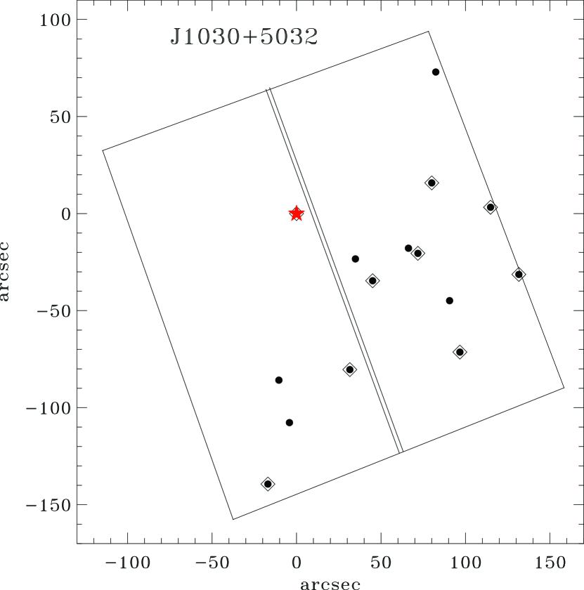
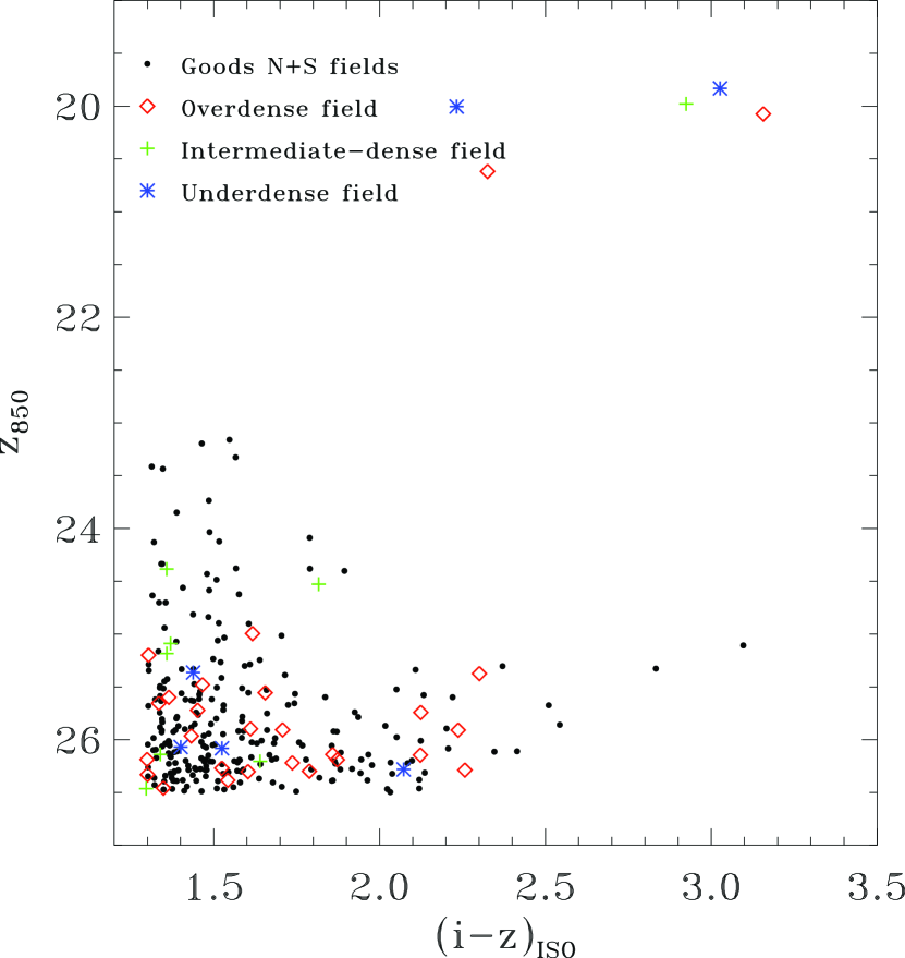
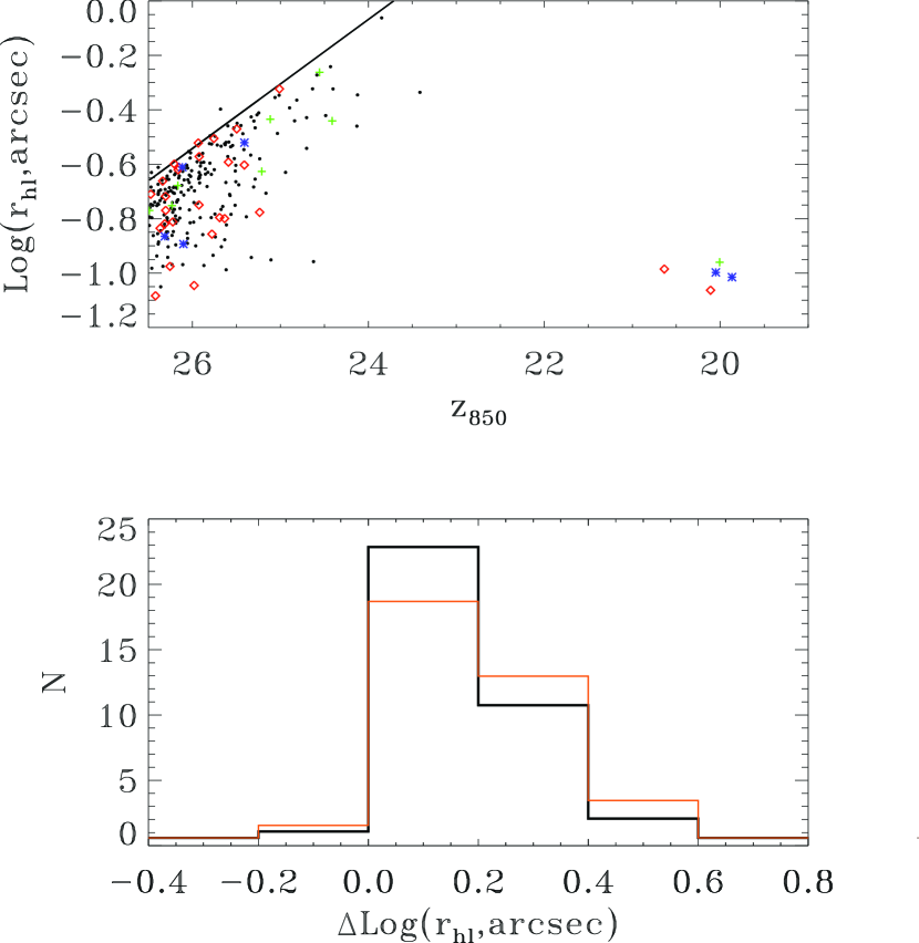
Figure 6 shows substantial spatial clustering of the $i_{775}$-dropout candidates in the J1030+0524 field: when the field is divided in half across the diagonal, almost all of the sources are in the south-west half of the field. This makes the excess in J1030+0524 even more significant. The color magnitude diagram of candidates listed in Table 3 is presented in Figure 7, showing that the overdense fields have fainter $i_{775}$-dropouts than GOODS. It is notable that Willott et al. (2005) in their less sensitive survey for $i_{775}$-dropouts around high-redshift SDSS QSOs, including J1030+0524, found no overdensities. The upper panel of Figure 8 shows half-light radius versus $z_{850}$ for the $i_{775}$-dropout candidates from GOODS and the QSO fields. There is an upper envelope to the size-magnitude relation, and the bottom panel of Figure 8 shows a histogram comparing the size distribution of GOODS and QSO field $i_{775}$-dropout half-light radii. It appears that the candidates in the overdense fields are more compact than those in GOODS, but this is not statistically significant.

4 DISCUSSION

Despite a complete reanalysis and a change in the type of SExtractor magnitudes used to compute the $i_{775}-z_{850}$ color for dropout selection (from AUTO to ISO mags), we confirm the overdensity in the J1030+0524 field reported in Stiavelli et al. (2005). The overdensity is significant not only in the counts by themselves but also in the color distribution. Indeed, the departure of the color distribution of J1030+0524 and J1630+4012 is in the sense of having an excess of red dropouts with precisely the colors that one would expect from objects at the redshift of the two QSOs. This makes the excess even more convincing.

One uncertain component of the comparison with GOODS is the possible contamination by low redshift and Galactic interlopers. Figure 9 shows the fraction of GOODS $i_{775}$-dropout objects selected by us but rejected when using the full GOODS $i_{775}$-dropout criteria including the $V_{606}$ data (Beckwith et al., 2006) to the number of GOODS $i_{775}$-dropouts selected by our criteria vs. the $i_{775}-z_{850}$ color. At $i_{775}-z_{850}>1.7$, where the excess of $i_{775}$-dropouts is large in the J1030+0524 and J1630+4012 fields, there is less than 15% contamination from potential foreground objects. Statistically, the full GOODS criteria would remove more objects from GOODS than from the J1030+0524 or J1630+4012 field because the latter have a redder color distribution. Thus, we do not think that the detected excess is due to interloper contamination.

In order to understand how unusual it is to identify this distribution of over- and underdensities, we consider the number of $i_{775}$-dropouts identified in 30 distinct and non-overlapping ACS fields in GOODS. Figure 10 presents the resulting histogram of the number of $i_{775}$-dropouts identified per unique GOODS ACS field using the S1 and the S2 selection criteria. These distributions are reasonably well fit by Poisson distributions with a mean of 6.5 (3.13) $i_{775}$-dropouts per ACS field for the S1 (S2) selection criteria. Using these distributions from GOODS, we create 10,000 Monte Carlo (MC) quintuplets, where each MC quintuplet is generated by randomly selecting five independent numbers of $i_{775}$-dropouts, each corresponding to a single ACS field. We then test how many MC quintuplets have the counts we have observed. For the S1, we find that only $0.06\pm 0.02$% of the MC quintuplets have exactly two overdense and two underdense fields. For the S2, this probability is only $0.03\pm 0.09$%. For the S3, six $i_{775}$-dropouts in one ACS field is the maximum number among the 30 ACS fields in GOODS so any MC quintuplets cannot be generated to have more than six $i_{775}$-dropouts. However, since one QSO field has 10 $i_{775}$-dropouts, we have zero probability for S3. The error bars on these probabilities are calculated by considering variations between 10 independent subsets of 1,000 MC quintuplets. This comparison to GOODS empirical dropout statistics suggests that the QSOs are indeed affecting their environments.

Estimating the likelihood of the counts observed in our fields on the basis of the $i_{775}$-dropout count distribution in GOODS is not entirely appropriate as even GOODS is affected by cosmic variance because within both the CDFS and the HDFN, the ACS fields are all adjacent. We can use the conservative model of cosmic variance of Trenti & Stiavelli (2008) to estimate the likelihood of our detected counts. This model is based on extended Press-Schechter theory as well as synthetic catalogs extracted from N-body simulations of structure formation. In this case, we establish the probability with $10^{6}$ MC quintuplets. We find that the likelihood of a MC quintuplet matching our observed distribution of over- and underdense fields using the S1 criteria is $0.9\pm 0.08\%$. S2 has a likelihood of $0.3\pm 0.05\%$, and S3 has a likelihood of $0.8\pm 0.09\%$. This result is less significant than that derived from the GOODS distribution, but it is comforting that the significance does not decrease when using samples with more stringent color or S/N selections. Thus, while we cannot claim for our overall sample a very significant detection of a discrepancy from a distribution dominated by cosmic variance alone, our distribution remains unlikely at the 99% level.

A criticism to this type of analysis is that these are not a-priori probabilities as we knew the outcome of the experiment before carrying out the statistical tests. This is only partly correct because the main idea of the HST proposal was indeed to look for overdensities or underdensities compared to the field even though the statistical test was not specified. Moreover, it is possible to design an experiment that does not depend as much on the observed counts, namely to evaluate the probability that out of the five fields only one is within one (Poissonian) $\sigma$ of the mean, i.e. within $8.08\pm 2.84$ for selection S1, within $3.95\pm 1.99$ for selection S2, or within $2.96\pm 1.72$ for selection S3. Here the formal Poisson $\sigma$ is used only to define an inner interval and has no attached probability significance. Probabilities are estimated by comparing how our observed object count distribution compares to that expected from cosmic variance. We find that the probability of finding no more than one out of five fields in the inner interval is of 20% for S1, 4% for S2, and 5.8% for S3. The same a priori test based on the observed counts distribution in GOODS would give a probability of finding no more than one object in the inner interval of 1.5% for S1, 0.4% for S2, and 1.5% for S3. This reinforces the view that the QSO fields have a distribution of $i_{775}$-dropout counts broader than what is expected by cosmic variance alone.

5 CONCLUSIONS

Summarizing our results, we find two fields where the numbers of $i_{775}$-dropout galaxies and their $i_{775}-z_{850}$ color distributions are significantly different (at 99% confidence) than the averages for galaxies selected in the same way from GOODS fields. When we look at the distribution of all five fields, we find that it is likely (at $80-96$% confidence level, depending on selection and specific statistical test) that the distribution of counts in the QSO fields is broader than that of GOODS and cannot be explained by cosmic variance alone.

We now discuss the possible implications of our results assuming that the departure from the expected distribution of field $i_{775}$-dropouts is indeed real. The fact that we observe both overdensities and underdensities is somewhat puzzling. We know that QSOs at $z=6$ are very rare objects and are most likely associated with overdensities on large scales. Tracing a pencil beam with the area of an ACS field through a cold dark matter (CDM) simulation box with the method of Trenti & Stiavelli (2008), we do not find correlations over $\Delta z\geq 0.3$. This is not surprising as $\Delta z=0.3$ corresponds to about 90 Mpc $h^{-1}$ at $z\sim 6$ and on those scale the CDM power spectrum predicts a value of the mass fluctuation $\sigma_{M}$ many orders of magnitude lower than the value that can be associated with the QSO itself. From this point of view, the redshift range probed by $i_{775}$-dropouts spans at least three uncorrelated volumes.

A QSO at $z\sim 6$ is expected to live in the most massive halos within $\approx$ Gpc³ comoving volumes, with masses of the order of $\approx 4\times 10^{12}h^{-1}M_{\sun}$ (e.g., Springel et al., 2005). Thus the dark matter halo mass function in the vicinity of the QSO halo will be biased by the presence of a rare overdensity (e.g., Barkana & Loeb, 2004). To quantify the impact of the QSO on the expected number counts in its immediate neighborhood we use the model of Munoz & Loeb (2007). From their Fig. 4 we derive that around the QSO there should be between 6 and 7 $i_{775}$-dropouts living in dark halos of mass $>5\times 10^{10}h^{-1}M_{\sun}$ taking into account an assumed duty cycle of 0.25 for LBGs. The duty cycle is used to establish a halo mass scale for the observed galaxies by requiring that the number of halos of the required mass be equal to the number of objects divided by the duty cycle. Adopting a duty cycle allows us to determine a mass scale from the number of objects and to avoid using the ill-measured M/L of galaxies at z ${\>\hbox to0.0pt{\raise 2.0pt\hbox{$>$}\hss}\lower 3.0pt\hbox{$\sim$}\>}6$. However, the results do not depend critically on the choice of duty cycle for range between 1 and 0.1. Our fields do not probably reach a depth that allows us to probe these halo masses with high completeness, but still we would expect to detect 2-3 of such LBGs or more if the “duty cycle” were higher.

In this light, deficits in the number of $i_{775}$-dropout candidates are surprising. Indeed 2/3 of the expected objects are in uncorrelated volumes and should not be affected by the presence of the QSO. The one third affected by the QSO now becomes a very small number and detecting a deficit in any single field is generally going to be statistically insignificant. It is interesting to note that at the time this project was planned the expected number of $i_{775}$-dropouts in GOODS was thought to be higher (e.g., Dickinson et al., 2004) so that a deficit would have been better quantifiable. Despite these considerations, the fact remains that we do seem to detect fields that have a deficit of $i_{775}$-dropout counts compared to the field. If we really had physical overdensities and physical underdensities near the QSO, what would be the origin of this effect? One possible explanation is that two physical mechanisms are simultaneously at play: the density of halos near the QSO is indeed higher but feedback by the QSO prevents many of these halos from becoming galaxies. The H II regions generated by luminous quasars can affect the formation and clustering of galaxies. Wyithe et al. (2005) derived H II size from displacement of quasar host galaxy redshift and the Gunn-Peterson trough redshift. The H II region size of the QSO J1030+0524 is the largest of the five quasars but the second overdense field, J1630+4012 and the most underdense field, J1306+0356, have very similar H II region sizes. The field with density comparable to GOODS, J1048+4637, has the smallest H II region size.

Thus, we find no evident correlation between density of $i_{775}$-dropouts and H II region size. This may or may not be significant as H II region sizes are roughly correlated with the luminosity of the quasars and their lifetimes; the latter measurements are not very accurate. We see a weak trend between counts and QSO luminosity as the two faintest QSOs are the two overdense ones and the most luminous QSO is one of the underdense ones. However, the most underdense QSO field(J1306+0356) is the third luminous QSO and within 0.04 mag from that of the most overdense (J1030+0524). On the basis of these considerations we conjecture that the suppression of galaxy formation which we may be witnessing could be the result of percolation of ionized Hydrogen bubbles. This would make it dependent, but not uniquely driven, by the QSO properties. Clearly it would be desirable to study these effects with better statistics.

Interestingly, Maselli et al. (2008), with an entirely different method, find conclusion similar to ours: namely, that J1630+4012 is overdense while J1148+5251 and J1306+0356 are underdense. They also find an overdensity around SDSS J0836+0054, also found to be overdense by Zheng et al. (2006). Maselli et al. (2008) predict that ionizing radiation from clustered galaxies for J1630+4012 exceeds the one from the quasar by a factor of five. We estimate the ionizing flux of our candidates. The total UV flux observed by summing the $z_{850}$ photometry from all of our $i_{775}$-dropout candidates is 7.0% and 8.5% of the quasar flux in $z_{850}$ for J1030+0524 and J1630+4012, respectively. For any reasonable spectral energy distribution, the excess is too small to affect the ionizing contributions. In order to have an influence at this level of overdensity, the excess should span a much larger area than that provided here. Clearly to further clarify these findings, we would need a larger sample as well as more extended data over overdense fields.

Table 1: Exposure times (in seconds) of QSO fields

Quasar Field	RA(J2000)	DEC(J2000)	Redshift	Exptime(F775W)	Exptime(F850LP)
J1030+0524	10 30 27.10	05 24 55.0	6.28	5840	11330
J1048+4637	10 48 45.05	46 37 18.3	6.23	6130	11770
J1148+5251	11 48 16.64	52 51 50.3	6.40	6180	11950
J1306+0356	13 06 08.26	03 56 36.3	5.99	5870	11340
J1630+4012	16 30 33.00	40 12 09.6	6.05	5980	11580

Table 2: Number of $i_{775}$-dropouts and Poisson error by S/N ratio and color limit

Field	S1	S2	S3
GOODS	$8.08\pm 2.84$	$3.95\pm 1.99$	$2.96\pm 1.72$
J1030+0524	$14\pm 3.74$	$8\pm 2.83$	$10\pm 3.16$
J1048+4637	$8\pm 2.83$	$2\pm 1.41$	$4\pm 2.00$
J1148+5251	$3\pm 1.73$	$2\pm 1.41$	$0\pm 0.00$
J1306+0356	$1\pm 1.00$	$0\pm 0.00$	$1\pm 1.00$
J1630+4012	$11\pm 3.32$	$8\pm 2.83$	$5\pm 2.24$

Note. — These numbers do not include the target quasars. The GOODS number has been normalized to the size of a single ACS field.

Table 3: Candidates with $i_{775}-z_{850}>1.3$ and S/N$>5$

Object	RA(J2000)	DEC(J2000)	$z_{850}$	$S/N(z_{850}$)	S/N($i_{775}$)	$i_{775}$-$z_{850}$	$r_{hl}$(arcsec)	S/G
A1	10 30 21.03	05 24 10.13	26.19	6.19	3.30	1.30	0.15	0.02
A2	10 30 21.57	05 26 07.94	26.33	6.17	2.96	1.30	0.15	0.98
A3	10 30 24.76	05 24 31.65	25.20	11.94	5.88	1.30	0.17	0.03
A4	10 30 27.79	05 24 31.65	25.66	10.47	4.91	1.33	0.16	0.02
A5	10 30 27.37	05 23 07.30	25.60	8.81	4.89	1.36	0.16	0.03
A6	10 30 22.66	05 24 37.16	25.72	8.63	1.85	1.45	0.31	0.29
A7	10 30 22.28	05 24 34.51	26.27	5.64	1.79	1.52	0.19	0.19
A8	10 30 24.98	05 23 34.62	26.38	9.63	3.59	1.54	0.08	0.97
A9	10 30 19.41	05 24 58.25	26.30	5.17	2.30	1.60	0.22	0.25
A10	10 30 18.28	05 24 23.65	25.90	8.78	0.38	1.61	0.30	0.78
A11	10 30 20.62	05 23 43.63	25.56	8.65	2.69	1.66	0.26	0.01
A12	10 30 28.23	05 22 35.64	26.22	9.41	2.55	1.74	0.11	0.85
A13	10 30 24.08	05 24 20.40	25.74	9.05	2.59	2.12	0.14	0.02
A14	10 30 21.73	05 25 10.81	25.37	9.18	1.28	2.30	0.25	0.02
QSO J1030+0524	10 30 27.09	05 24 55.00	20.07	461.80	45.97	3.16	0.09	0.85
B1	16 30 40.71	40 11 17.38	26.47	6.11	3.12	1.35	0.20	0.01
B2	16 30 37.55	40 11 55.94	25.98	13.55	7.07	1.44	0.09	0.98
B3	16 30 40.55	40 12 20.01	25.50	9.90	4.35	1.47	0.34	0.02
B4	16 30 40.51	40 12 43.29	25.01	13.49	4.57	1.62	0.47	0.02
B5	16 30 26.62	40 13 31.02	25.92	7.68	3.12	1.71	0.27	0.01
B6	16 30 27.90	40 11 16.90	26.31	7.73	3.46	1.79	0.15	0.02
B7	16 30 43.82	40 11 59.92	26.16	7.88	1.41	1.86	0.25	0.01
B8	16 30 26.87	40 12 45.88	26.21	7.31	0.45	1.87	0.25	0.02
B9	16 30 41.11	40 13 5.89	26.16	7.84	0.80	2.12	0.24	0.01
B10	16 30 42.48	40 12 14.05	25.93	9.46	2.47	2.24	0.18	0.02
B11	16 30 36.99	40 13 9.27	26.30	10.28	1.51	2.26	0.17	0.02
QSO J1630+4012	16 30 33.85	40 12 9.48	20.63	338.76	83.90	0.10	0.10	0.87
C1	10 48 52.34	46 36 12.29	26.46	5.62	2.30	1.30	0.17	0.83
C2	10 48 42.39	46 36 40.56	26.14	6.36	1.77	1.34	0.21	0.78
C3	10 48 52.48	46 37 11.05	24.38	12.80	7.88	1.36	0.36	0.02
C4	10 48 53.47	46 35 55.93	25.19	8.45	4.60	1.36	0.24	0.02
C5	10 48 42.21	46 38 20.34	25.09	10.65	3.02	1.37	0.37	0.17
C6	10 48 47.62	46 36 01.41	26.21	5.60	2.10	1.64	0.18	0.11
C7	10 48 42.13	46 38 21.58	24.53	12.42	1.98	1.82	0.55	0.01
QSO J1048+4637	10 48 45.22	46 37 17.92	19.98	303.81	61.30	2.92	0.11	0.86
D1	11 48 07.93	52 51 59.32	26.07	7.03	3.52	1.40	0.13	0.84
D2	11 48 15.41	52 51 07.14	26.08	6.72	1.88	1.52	0.25	0.49
D3	11 48 20.29	52 53 04.22	26.28	7.61	1.59	2.07	0.14	0.01
QSO J1148+5251	11 48 16.74	52 51 50.11	19.83	450.77	66.60	3.03	0.10	0.85
E1	13 06 2.08	03 56 04.70	25.36	8.69	-0.19	1.44	0.30	0.13
QSO J1306+0356	13 06 08.22	03 56 25.92	20.00	272.52	97.22	2.23	0.10	0.85

Figure 1: Distributions of the number of objects versus magnitude and color, comparing objects in the SDSS J1030+5032 field (solid histograms) to those in the GOODS field (dotted histograms). The GOODS counts are normalized to the area of the quasar field ($\sim$11.3 arcmin²). Panel (a) shows the total counts vs. $z_{850}(AUTO)$ of all objects with no selection criteria applied. Panel (b) shows the total counts vs. $i_{775}$-$z_{850}$ of all objects with no selection criteria applied. Panel (c) shows the candidates with $i_{775}$-$z_{850}>1.5$; the brightest object is the target QSO. Panel (d) shows the number of objects redder than a given $i_{775}$-$z_{850}$, excluding the target QSO, with the GOODS counts renormalized to the QSO counts at $0.9<i_{775}$-$z_{850}<1.0$.

Figure 2: Same as Fig 1. for J1630+4012

Figure 3: Same as Fig 1. for J1048+4637

Figure 4: Same as Fig 1. for J1148+5251

Figure 5: Same as Fig 1. for J1306+0356

Figure 6: The spatial distribution of $i_{775}$-dropouts redder than 1.3 (circles) and redder than 1.5 (open squares) for S/N$>5$ in the J1030+0524 field. The star represents the QSO SDSS J1030+0524. The axes of x and y are in arcseconds and they are relative to the QSO position. East is to the left and north is up.

Figure 7: Color-magnitude distribution of $i_{775}$-dropouts, selected using S1 criteria, in GOODS (small black dots) and the five QSO fields. The overdense QSO fields are indicated with red diamonds, the underdense QSO fields are indicated with blue asterisks, and the intermediate density QSO field is indicated with green crosses. The brightest objects, with $z_{850}{\>\hbox to0.0pt{\raise 2.0pt\hbox{$<$}\hss}\lower 3.0pt\hbox{$\sim$}\>}21$, are the QSOs.

Figure 8: The upper panel shows half-light radii of $i_{775}$-dropout candidates (S1 sample) with respect to $z_{850}$ magnitude for excess (red diamonds), deficit (blue asterisks), and intermediate (green crosses) density fields, as well as for GOODS (black dots). The five bright objects at $z_{850}{\>\hbox to0.0pt{\raise 2.0pt\hbox{$<$}\hss}\lower 3.0pt\hbox{$\sim$}\>}21$ are the QSOs. The solid line is fitted to the upper limit of the logarithmic radii of the objects in GOODS. The lower panel shows the histogram of the distances from the upper envelope on the upper panel to the logarithmic radii data of the all five QSO fields (orange line) and the GOODS field (black line) along the axis of ordinates. The histogram of GOODS is normalized to the area of the QSO fields.

Figure 9: The ratio of the number of GOODS $i_{775}$-dropouts selected by us (S1) but rejected by the full GOODS selection criteria, including S/N$(V_{606})<2.0$ or $V_{606}-z_{850}<2.8$ (Beckwith et al., 2006) to the number of GOODS $i_{775}$-dropouts selected by our criteria.

Figure 10: Histograms (upper panels) of the number of $i_{775}$-dropouts per ACS field in the GOODS North and South (Solid lines) for S1 sample (on the left) and S2 sample (on the right). Poisson distributions (dashed lines) with a mean of 6.5 for $i_{775}-z_{850}>1.3$ and 3.13 for $i_{775}-z_{850}>1.5$ are fitted. The 30 ACS fields are overlaid in the whole GOODS field. The bottom panels show cumulative distributions from the histograms

References

- Barkana & Loeb (2004) Barkana, R., & Loeb, A. 2004, ApJ, 609, 474
- Barth et al. (2003) Barth, A. J., Martini, P., Nelson, C. H., & Ho, L. C. 2003, ApJ, 594, L95
- Becker et al. (2001) Becker, R. H., et al. 2001, AJ, 122, 2850
- Beckwith et al. (2006) Beckwith, S. V. W., et al. 2006, AJ, 132, 1729
- Bertin & Arnouts (1996) Bertin, E., & Arnouts, S. 1996, A&AS, 117, 393
- Bolton & Haehnelt (2007) Bolton, J. S., & Haehnelt, M. G. 2007, MNRAS, 374, 493
- Bouwens et al. (2007) Bouwens, R. J., Illingworth, G. D., Franx, M., & Ford, H. 2007, ApJ, 670, 928
- Bunker et al. (2004) Bunker, A. J., Stanway, E. R., Ellis, R. S., & McMahon, R. G. 2004, MNRAS, 355, 374
- Cen (2003) Cen, R. 2003, ApJ, 591, 12
- Ciardi et al. (2003) Ciardi, B., Ferrara, A., & White, S. D. M. 2003, MNRAS, 344, L7
- Dickinson et al. (2004) Dickinson, M., et al. 2004, ApJ, 600, L99
- Djorgovski (1999) Djorgovski, S. G. 1999, The Hy-Redshift Universe: Galaxy Formation and Evolution at High Redshift, 193, 397
- Djorgovski et al. (2001) Djorgovski, S. G., Castro, S., Stern, D., & Mahabal, A. A. 2001, ApJ, 560, L5
- Djorgovski et al. (1999) Djorgovski, S. G., Odewahn, S. C., Gal, R. R., Brunner, R. J., & de Carvalho, R. R. 1999, Photometric Redshifts and the Detection of High Redshift Galaxies, 191, 179
- Djorgovski et al. (2003) Djorgovski, S. G., Stern, D., Mahabal, A. A., & Brunner, R. 2003, ApJ, 596, 67
- Efstathiou & Rees (1988) Efstathiou, G., & Rees, M. J. 1988, MNRAS, 230, 5P
- Fan et al. (2001) Fan, X., et al. 2001, AJ, 122, 2833
- Fan et al. (2003) Fan, X., et al. 2003, AJ, 125, 1649
- Fan et al. (2006) Fan, X., et al. 2006, AJ, 132, 117
- Fruchter & Hook (2002) Fruchter, A. S., & Hook, R. N. 2002, PASP, 114, 144
- Giavalisco et al. (2004) Giavalisco, M., et al. 2004, ApJ, 600, L93
- Gnedin (2004) Gnedin, N. Y. 2004, ApJ, 610, 9
- Gnedin & Ostriker (1997) Gnedin, N. Y., & Ostriker, J. P. 1997, ApJ, 486, 581
- Gunn & Peterson (1965) Gunn, J. E., & Peterson, B. A. 1965, ApJ, 142, 1633
- Haiman & Holder (2003) Haiman, Z., & Holder, G. P. 2003, ApJ, 595, 1
- Kaiser (1984) Kaiser, N. 1984, ApJ, 284, L9
- Koekemoer et al. (2002) Koekemoer, A. M., Fruchter, A. S., Hook, R. N., & Hack, W. 2002, The 2002 HST Calibration Workshop : Hubble after the Installation of the ACS and the NICMOS Cooling System, Proceedings of a Workshop held at the Space Telescope Science Institute, Baltimore, Maryland, October 17 and 18, 2002. Edited by Santiago Arribas, Anton Koekemoer, and Brad Whitmore. Baltimore, MD: Space Telescope Science Institute, 2002., p.337, 337
- Komatsu et al. (2008) Komatsu, E., et al. 2008, ArXiv e-prints, 803, arXiv:0803.0547
- Lidz et al. (2006) Lidz, A., Oh, S. P., & Furlanetto, S. R. 2006, ApJ, 639, L47
- Malhotra et al. (2005) Malhotra, S., et al. 2005, ApJ, 626, 666
- Maselli et al. (2008) Maselli, A., et al. 2008, MNRAS, submitted
- McDonald & Miralda-Escudé (2001) McDonald, P., & Miralda-Escudé, J. 2001, ApJ, 549, L11
- Miralda-Escudé et al. (2000) Miralda-Escudé, J., Haehnelt, M., & Rees, M. J. 2000, ApJ, 530, 1
- Muñoz & Loeb (2008) Muñoz, J. A., & Loeb, A. 2008, MNRAS, 385, 2175
- Oesch et al. (2007) Oesch, P. A., et al. 2007, ApJ, 671, 1212
- Ouchi et al. (2005) Ouchi, M., et al. 2005, ApJ, 620, L1
- Schlegel et al. (1998) Schlegel, D. J., Finkbeiner, D. P., & Davis, M. 1998, ApJ, 500, 525
- Shapiro & Raga (2001) Shapiro, P. R., & Raga, A. C. 2001, Revista Mexicana de Astronomia y Astrofisica Conference Series, 10, 109
- Shull & Venkatesan (2007) Shull, M., & Venkatesan, A. 2007, ArXiv Astrophysics e-prints, arXiv:astro-ph/0702323
- Somerville et al. (2003) Somerville, R. S., Bullock, J. S., & Livio, M. 2003, ApJ, 593, 616
- Springel et al. (2005) Springel, V., et al. 2005, Nature, 435, 629
- Steidel et al. (2003) Steidel, C. C., Adelberger, K. L., Shapley, A. E., Pettini, M., Dickinson, M., & Giavalisco, M. 2003, ApJ, 592, 728
- Stiavelli et al. (2005) Stiavelli, M., et al. 2005, ApJ, 622, L1
- Stiavelli et al. (2004) Stiavelli, M., Fall, S. M., & Panagia, N. 2004, ApJ, 610, L1
- Trenti & Stiavelli (2007) Trenti, M., & Stiavelli, M. 2007, ApJ, 667, 38
- Trenti & Stiavelli (2008) Trenti, M., & Stiavelli, M. 2008, ApJ, 676, 767
- Venemans et al. (2003) Venemans, B. P., Kurk, J. D., Miley, G. K., & Röttgering, H. J. A. 2003, New Astronomy Review, 47, 353
- White et al. (2003) White, R. L., Becker, R. H., Fan, X., & Strauss, M. A. 2003, AJ, 126, 1
- Willott et al. (2005) Willott, C.J., et al., 2005, in “Growing Black Holes”, ESO (Garching), Merloni et al. eds, (also astro-ph/0410306)
- Wyithe & Loeb (2003) Wyithe, J. S. B., & Loeb, A. 2003, ApJ, 588, L69
- Wyithe et al. (2005) Wyithe, J. S. B., Loeb, A., & Carilli, C. 2005, ApJ, 628, 575
- Yan & Windhorst (2004) Yan, H., & Windhorst, R. A. 2004, ApJ, 600, L1
- Zheng et al. (2006) Zheng, W., et al. 2006, ApJ, 640, 574
- Zombeck (1990) Zombeck, M.V. 1990, Handbook of Space Astronomy and Astrophysics (Cambridge University Press: Cambridge), p.77