Impurities in triangular lattice spin 1/2 antiferromagnet

Abstract

We study effects of nonmagnetic impurities in a spin-1/2 frustrated triangular antiferromagnet with the aim of understanding the observed broadening of ¹³C NMR lines in the organic spin liquid material $\kappa$-(ET)₂Cu₂(CN)₃. For high temperatures down to $J/3$, we calculate local susceptibility near a nonmagnetic impurity and near a grain boundary for the nearest neighbor Heisenberg model in high temperature series expansion. We find that the local susceptibility decays to the uniform one in few lattice spacings, and for a low density of impurities we would not be able to explain the line broadening present in the experiments already at elevated temperatures. At low temperatures, we assume a gapless spin liquid with a Fermi surface of spinons. We calculate the local susceptibility in the mean field and also go beyond the mean field by Gutzwiller projection. The zero temperature local susceptibility decays as a power law and oscillates at $2k_{F}$. As in the high temperature analysis we find that a low density of impurities is not able to explain the observed broadening of the lines. We are thus led to conclude that there is more disorder in the system. We find that a large density of point-like disorder gives broadening that is consistent with the experiment down to about $5$K, but that below this temperature additional mechanism is likely needed.

I Introduction

Spin liquid phases are some of the most interesting phases known to exist theoretically. However they are hard to achieve experimentally because interactions usually favor ordered phases. To achieve spin liquid we have to frustrate these interactions. Triangular lattice provides a natural way to do this. For the nearest neighbor antiferromagnetic Heisenberg model the frustration is not strong enough and the ground state is ordered. However, the order is weak, and it is likely that in the presence of appropriate additional interactions, spin liquid phases arise.

This work is motivated by the layered organic compound $\kappa$-(ET)₂Cu₂(CN)₃.Shimizu03 ; Kurosaki ; Kawamoto04 ; Shimizu06 ; Kawamoto06 ; McKenzie It contains ET molecules that pair up, each pair lies on sites of triangular lattice and has one electron less then the full filling. The material at ambient pressure is an insulator. Thus it is effectively a spin 1/2 antiferromagnet on the triangular lattice. While the Heisenberg exchange $J\approx 250$ K, the system shows no signs of ordering down to $32$ mK making it a good candidate for the spin liquid. There are likely additional interactions among spins, especially ring exchanges that are thought to be responsible for driving the system into the spin liquid.LiMing ; ringxch ; SSLee ; Nave What makes the appearance of such interactions natural is that under moderate pressure the $\kappa$-(ET)₂Cu₂(CN)₃ undergoes a transition to a superconductor at low temperature (and a metal at higher temperature), so there are significant virtual charge fluctuations present already in the insulator at ambient pressure.Shimizu03 ; Kurosaki Crudely, we can think of the system as a half-filled Hubbard model close to the Mott insulator - metal transition, and we can estimate that the ring exchange interactions in the effective spin model are strong, enough to destroy the magnetic order. ringxch ; Zheng ; LiMing An alternative explanation of the insulator in terms of inhomogeneous electron localization has also been suggested. Kawamoto04 ; Kawamoto06

The spin liquid phase remains enigmatic. Thermodynamic measurements show many gapless excitations in this charge insulator – at least as many as in a metal. One appealing proposal that captures some of the observed phenomenology is a state with spinon Fermi surface. ringxch ; SSLee ; Nave Other scenarios have also been suggested, Wang ; Galitski ; Qi ; Senthil particularly with the view towards low temperatures.

We are specifically interested in the ¹³C NMR measurements of the Knight shifts,Kawamoto04 ; Shimizu06 ; Kawamoto06 and what we can learn from these for the material and the spin liquid. The measurements effectively give a histogram of local magnetic susceptibility and are therefore a good probe of the magnetic properties. The experiment shows strong broadening of such histogram as one lowers the temperature. The width of the peak broadens by about a factor of 40 as the temperature is lowered from 250 K to roughly 1 K and saturates as the temperature is lowered further. The distribution of local susceptibilities can be produced by disorder, since the susceptibility can have various values as a function of distance from say an impurity. It is hard to imagine other mechanism producing a distribution (except spin glass, but no such behavior is observed). Therefore in this paper we investigate the effects of disorder on the spin system.

Unfortunately, not much is known about the impurities and their role in the insulating $\kappa$-(ET)₂Cu₂(CN)₃ at ambient pressure. At high pressure of 0.8 GPa, the material is a relatively clean metal with $k_{F}l\gtrsim 50-100$ and observable Shubnikov-deHaas oscillations. It is believed that the Cu²⁺ impurity concentration is very low,Shimizu03 less than 0.01%. There are quite possibly additional sources of disorder such as different local environments coming from different conformations of the ET molecules, Soto ; Miyagawa ; Wolter ; Maksimuk or from disorder in the insulating anion layers such as the disordered (CN)^- group.Geiser ; Komatsu ; Emge ; Kawamoto06 Analyzing the NMR experiments can then provide some understanding of the disorder, its strength, and role in the insulator phase. Taking up the Mott insulator picture as one viable candidate, where the insulator is primarily driven by electron-electron interactions, we set out to study models of non-magnetic disorder in a spin-1/2 system on the triangular lattice. We study progressively different kinds of disorder and analyze what each predicts about the local susceptibilities in turn.

This paper consists of two separate approaches: one, the high temperature series expansion, and the other, low temperature analysis assuming the system forms a spin liquid. High temperature series expansion is rather restricted by the range of temperatures and the types of models it can study, but for those models it gives exact results. We are able to calculate local susceptibilities of the nearest neighbor Heisenberg model on an arbitrary graph where all exchange couplings are the same. In particular, we can study triangular lattice with a missing site, with a boundary, or in the presence of a finite density of missing sites. The missing sites are models of nonmagnetic impurities, while the boundary is a model of grain boundary. We can go down to temperature of roughly $J/3$. In this range, the experiments already see broadening of the Knight shift distribution by about a factor of two and thus we can compare the calculated results to the experiments. Of course, the real material has interactions beyond the nearest neighbor since it is a spin liquid, but rough estimate can be made, especially given that multi-spin exchanges are less important at high temperatures.

At low temperatures we assume phenomenologically the system forms a spin liquid with Fermi sea of spinons (stabilized by additional interactions). We first analyze this in mean field where it reduces to free fermions hopping on the triangular lattice. The spin liquid can naturally accommodate nonmagnetic disorder in the spin model by the corresponding changes in the spinon hopping amplitudes. The full theory also contains a dynamical U(1) gauge field, SSLee ; LeeNagaosaWen ; Ioffe ; LeeNagaosa ; Polchinski ; Altshuler but this is hard to analyze directly. Instead, to go beyond mean field we study wavefunctions obtained by Gutzwiller projection of the mean field states. In one dimension, this can capture the full theory, while in two dimensions this is only an approximation but a reasonable one and dealing directly with physical spins.

Overall, we find that the local susceptibility decays rather quickly near an impurity and at small impurity densities such as $0.01\%$ of Cu our results are very far from explaining the experimental data – they would produce very sharp histograms as most of the sites are in the bulk. In the spin liquid phase, the local susceptibility has an oscillatory $2k_{F}$ component that decays with a power law envelope away from defects, so the impurities can be felt at larger distances, but the overall amplitude that we find is still small.

We then studied the system at high temperature near a boundary and in the presence of a larger density of missing sites. We also studied the system at low temperature in the mean field near a boundary, in the presence of a larger density of missing sites, and in the presence of random disorder on bonds which is either uniform or localized at a fraction of bonds. From this analysis it appears that the most likely scenario is the case of relatively large density of point-like disorder, where the linewidths broaden with lowering the temperature until the correlation length becomes comparable to the typical distance between defects. A puzzling feature is that with such fixed disorder we cannot reproduce the observed strong temperature dependence of the NMR lines as the temperatures are lowered further. On the other hand, such models in the metallic phase where we considered electrons with random on-site potentials match reasonably with the experiments under pressure, where the NMR linewidths remain unchanged with temperature.Kawamoto06 It could be also that the effective strength of disorder increases as the temperature is lowered in the insulator, perhaps because of the vanishing screening of charged impurities. Better understanding of the disorder in the $\kappa$-(ET)₂Cu₂(CN)₃ system is clearly needed.

A new triangular lattice spin liquid material EtMe₃Sb[Pd(dmit)₂]₂, Ref. Itou, , has rather similar phenomenology to that of the $\kappa$-(ET)₂Cu₂(CN)₃ and also appears to have significant NMR line broadening, which may thus be a common feature of gapless spin liquids. It would be interesting to compare both systems more.

Finally we would like to mention that we have performed similar analysis on Kagome antiferromagnet addressing the NMR line broadening in the candidate spin liquid material ZnCu₃(OH)₆Cl₂. Kagome_SL ; Kagome_NMR ; Kagome_Zn There, the disorder is relatively well understood experimentally and is estimated to be about $5\%$ vacancies. Our calculationskagome_w_vacancies in this case compare sensibly with the experiment.

II Summary of the Experimental Inhomogeneous Line Broadening

In what follows, we calculate local susceptibility in spin models with nonmagnetic disorder. To set the stage, we summarize the main experimental findings in the form convenient for judging theoretical results. A direct comparison with the experiments is to look at the width of the local susceptibility histograms relative to the average susceptibility. In the model calculations the bulk susceptibility is roughly the location of the histogram peak, while in the experimental plots we should also be aware of the chemical shifts. The referencing to the average susceptibility is justified since in the $\kappa$-(ET)₂Cu₂(CN)₃ this remains roughly unchanged around $\bar{\chi}=5\cdot 10^{-4}$ emu/mol in a wide temperature range between 300 K and 30 K and then decreases somewhat to a value around $\bar{\chi}=3\cdot 10^{-4}$ emu/mol at 1 K. Also, the bulk values can be quantitatively reproduced by suitable choices of the model parameters such as $J$ in the high-temperature series studyShimizu03 ; Zheng or the spinon hopping amplitude in the spin liquid model (see Sec. IV).

Refs. Kawamoto04, ; Shimizu06, ; Kawamoto06, show the NMR lines plotted versus shifts from tetramethylsilane (TMS), in parts per million (ppm). For the more strongly coupled ¹³C whose hyperfine coupling constant is $0.21$ Tesla/($\mu_{B}$ dimer), the susceptibility of $\bar{\chi}=5\cdot 10^{-4}$ emu/mol corresponds to $\delta B/B=1.8\cdot 10^{-4}=180$ ppm Knight shift. Thus a 20 ppm shift corresponds to roughly a 10% relative change in the susceptibility at higher temperatures and a somewhat larger relative change at lower temperatures. Reading from the experiments, the full width at half maximum (FWHM) of the line measured in such relative terms increases from about 10% at 300 K to about 20-30% at 50 K to about 50-60% at 10 K, and then increases steeply to about 300% at 1 K and saturates around this value at still lower temperatures. One can appreciate the dramatic broadening directly from the line shapes in Refs. Kawamoto04, ; Shimizu06, ; Kawamoto06, , where the distance of this line from the origin sets a natural scale since the Knight shift and the chemical shift are comparable. (Note that to see the inhomogeneous Knight shifts over the intrinsic linewidths the experiments are done in large fields of order 8 Tesla; this may be inducing more significant ground state modifications, while in this work we focus on the linear response susceptibilities and their distributions.)

We note that the broadening first sets in gradually coming from high temperatures. The line is already 20-30% broad at $T=50~{}{\rm K}\sim J/5$ , which we can hope to understand quantitatively using reliable high-temperature series approach. It further broadens by about a factor of two to three in the region 50 K to 5-10 K where we expect the spin liquid approach to become applicable. We now present these two studies.

III High Temperature Series Expansion

We consider spin $1/2$ nearest neighbor anti-ferromagnetic Heisenberg model on triangular lattice. Local spin susceptibility at site $i$ is given by

$$\chi_{\rm loc}(i)=\frac{(g\mu_{B})^{2}\langle S_{i}^{z}S_{\rm tot}^{z}\rangle}{k_{B}T}~{},$$ (1)

where $S_{\rm tot}^{z}=\sum_{j}S_{j}^{z}$. We calculate $\chi$’s in the high temperature series expansions in the presence of nonmagnetic impurities treated as missing sites (vacancies), and also near an open boundary which is a model for a grain boundary.

The expansion is performed to the 12-th order in $J$ (or 13-th order in $1/T$) using the linked cluster expansion.OitmaaBook The outline of the procedure is as follows. We generate all abstract graphs up to desired size. Then we generate all subgraphs of these graphs, keeping track of the location of each subgraph in the graph.

We calculate the local susceptibility for each graph at each point of the graph. Then we subtract all the subgraphs of each graph as needed in the linked cluster expansion to get the contribution this graph would give when embedded into lattice. The local susceptibility on any lattice can be calculated by creating all possible embeddings of all graphs and adding their contributions at every site. In this general formulation the lattice does no need to be regular, it can be any connected graph. In particular this procedure applies to the triangular lattice with a missing site, with a finite density of missing sites, or with a boundary. In practice, for the single impurity case, we consider all the graphs containing the impurity and subtract their contribution from the uniform susceptibility. Similar procedure is used in the case with the boundary. In the end, we obtain exact $1/T$ series expansion for the system with such disorder.kagome_w_vacancies

After obtaining the series, we extend it beyond the radius of convergence using the method of Pade approximants. We use [5,6], [5,7], [6,6], [6,7] and expand in variable $1/(T+\alpha)$ where $\alpha$ is usually 0.08 as in Ref. Elstner93, . Depending on $\alpha$ one might get a pole in the expression, and hence divergence in susceptibility even at relatively large temperature. This usually happens say in one of the approximants while the others still overlap. At low enough temperatures they start diverging and we take that as a point where the approximation stops being valid. Different values of $\alpha$ are tried, and sometimes it is possible to tune to a value where all the curves overlap completely to a much lower temperature, but that is a pathology, probably indicating that the polynomials are all the same. For other values of $\alpha$ the curves usually start to diverge from each other at around the same temperature.

III.1 Point Impurity and Nonzero Density of Impurities

The coefficients of the susceptibility of the first five nearest neighbors near the impurity are in Table 1. The corresponding local susceptibilities along with the uniform susceptibility are plotted in Figure 1. We see that the local susceptibility decays to the uniform one in few lattice spacings. This is consistent with calculated very short correlation length in Ref. Elstner93, . The deviation of the near-neighbor local susceptibility from the uniform value reaches roughly $15\%$ at $T\approx J/3$.

Table 1: Series coefficients $a_{n}$ of $\chi=\frac{g^{2}\mu_{B}^{2}}{T}\sum_{n=0}\frac{a_{n}}{4^{n+1}(n+1)\text{!}}(\frac{J}{T})^{n}$ for susceptibility $\chi_{\rm uniform}$ of the pure triangular lattice and for the five closest neighbors $\chi_{i}$ of nonmagnetic impurity as indicated in Figure 1. The coefficients for the uniform susceptibility agree with Ref. Elstner93, .

n	$\chi_{\rm uniform}$	$\chi_{1}$	$\chi_{2}$	$\chi_{3}$	$\chi_{4}$	$\chi_{5}$
0	1	1	1	1	1	1
1	-12	-10	-12	-12	-12	-12
2	144	108	132	138	144	144
3	-1632	-1248	-1312	-1400	-1560	-1608
4	18000	15840	13840	13320	14880	16160
5	-254016	-237024	-235776	-213984	-189168	-192000
6	5472096	4144000	5539968	5817504	5084464	4564560
7	-109168128	-73210624	-93128960	-109647744	-123994240	-118354560
8	818042112	1133266176	222006528	112173696	913327488	1312247808
9	17982044160	-18170275840	11644656640	30128806400	38868680960	28664414720
10	778741928448	581215033344	1535178191360	1512448745984	328581324544	-104688021504
11	-90462554542080	-21239974981632	-84715204509696	-115649955864576	-118987461639168	-96786926315520
12	829570427172864	215676565092352	-788032311226368	-332026092103680	2149211723363328	2738259718125568

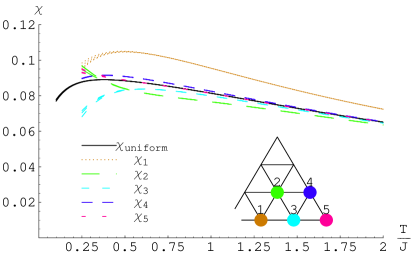
Figure 1: [Color online] The uniform susceptibility and the local susceptibilities at the first five inequivalent neighbors of nonmagnetic impurity (missing site). The four curves for each $\chi_{i}$ are the Pade approximants [5,6],[5,7],[6,6],[6,7]. $\chi$ is in units of $(g\mu_{B})^{2}/J$.

We would like to see if the observed NMR lines can be explained from a finite density of such impurities. The prediction is obtained by plotting the histogram of susceptibilities. First we note that at $T\sim 100{\rm K}\sim J/3$ the experimental lines are spread by about $\pm 10\%$ which is roughly equal to the calculated deviation of the local susceptibility of the nearest neighbors from the uniform susceptibility. The experimental curves have a significant weight spread over this width, and so if the calculated curves are to explain them, the first few nearest neighbors of impurities would have to form a sizable fraction of the total number of sites. Ref. Shimizu03, suggests that the system contains about one Cu impurity in ten thousand which gives about $0.4\%$ fraction for the nearest neighbors up to $\chi_{5}$ in Fig. 1 and hence it is very far from explaining the experimental lines – it would predict very sharp histograms.

One possible explanation of this discrepancy is the fact that the Heisenberg model is not entirely adequate because it would eventually predict ordering at low temperatures, which is not observed in experiments, and so there are additional interactions. Indeed, Ref. ringxch, proposed that ring exchanges are important to stabilize the spin liquid phase. However, since these interactions are still short-range, the volume fraction of sites that are affected by vacancies at these temperatures is still small, so low impurity density cannot fit the observed data.

A different more likely explanation is that there are more impurities or more disorder in the system. One possible source of disorder is from extended defects such as grain boundaries, and in the next section we consider the susceptibility near a boundary. Other possible source is from the ethylene group disorder in the ET molecules which is thought to be important in a related $\kappa$-(ET)₂Cu[N(CN)₂]Br material. Soto ; Miyagawa ; Wolter ; Maksimuk This can give rise to a large density of point perturbations which are mild but present everywhere. Other possible source is disorder in the (CN)^- groups in the insulating anion layers. Geiser ; Komatsu ; Emge We currently do not know much about the presence and magnitude of such perturbations in the spin liquid $\kappa$-(ET)₂Cu₂(CN)₃ material.

To simulate a case of a large density of point-like disorder, we study the system in the presence of a 5% of missing sites. Realistic point-like disorder is probably of a different nature, but vacancies is all we can do in the systematic high temperature expansion. However we hope the basic features of the histogram would be similar. The result is shown in the Fig. 2. Due to a large number of diagram imbeddings we were able only to go to the 11th order in $J$ (rather than $12$-th as above) on a $20\times 20$ lattice and reliably only down to $T\sim 0.5J$. The error on the histogram values is roughly $\pm 20\%$. Crudely, we see two sets of peaks in Fig. 2: The one on the right is associated with the nearest neighbors of the impurities while the one on the left with the rest of the sites. The finer features are associated with sites at different positions with respect to several impurities.

As we have already mentioned, the nearest neighbor susceptibility is different from the the uniform one by about 10%, which is roughly similar to the broadening of the NMR line at $T\sim 100-50$ K. However the temperature dependence of $\chi_{1}-\chi_{\rm uniform}$ is also weak, see Fig. 1. In the case with very low density of impurities such as $0.01\%$ Cu, besides having this value only at very few sites, it would not give broadening of the lines. In the case of $5\%$ of impurities, Fig. 2, this corresponds to the distance between the two sets of peaks not changing significantly with temperature. On the other hand the (set of) peaks themselves visibly broaden more. Remembering that here we plot histograms corresponding to the “ideal” system (i.e., with only Heisenberg exchanges and vacancies, and not including other interactions and sources of line widths), few percent of impurities can indeed produce reasonably broadened lineshapes at these elevated temperatures.

Figure 2: The histogram of local susceptibilities for a $20\times 20$ triangular lattice sample with 5% randomly placed vacancies, obtained from the high temperature series expansion to 11-th order in $J$. $\chi$ is in units of $(g\mu_{B})^{2}/J$.

III.2 Line Impurity

In this subsection we consider pure triangular lattice near a boundary and calculate susceptibility at various distances from the boundary. The coefficients of the uniform susceptibility and of the local susceptibility at the first five closest inequivalent sites are in Table 2. The corresponding plots are in Figure 3.

Table 2: Series coefficients $a_{n}$ of $\chi=\frac{g^{2}\mu_{B}^{2}}{T}\sum_{n=0}\frac{a_{n}}{4^{n+1}(n+1)\text{!}}(\frac{J}{T})^{n}$ for susceptibility $\chi_{\rm uniform}$ of the pure triangular lattice and for the five closest inequivalent neighbors $\chi_{i}$ to a boundary as indicated in Figure 3.

n	$\chi_{\rm uniform}$	$\chi_{1}$	$\chi_{2}$	$\chi_{3}$	$\chi_{4}$	$\chi_{5}$
0	1	1	1	1	1	1
1	-12	-8	-12	-12	-12	-12
2	144	72	120	144	144	144
3	-1632	-752	-896	-1440	-1632	-1632
4	18000	8640	5120	9040	16080	18000
5	-254016	-103488	-108960	-37248	-127296	-230976
6	5472096	1497440	3972864	2808736	1342432	3429216
7	-109168128	-29967872	-58795776	-109978368	-46504448	-21990912
8	818042112	553745664	-912840192	598482432	1331324928	-895304448
9	17982044160	-4034237440	35460869120	74136878080	-6674631680	-1900426240
10	778741928448	-38283289088	1453883081728	-796283040256	-765905530368	2445141614080
11	-90462554542080	-6599243882496	-88646526167040	-131119323998208	1918538846208	-58857804742656
12	829570427172864	433688769173504	-1170019148326912	3744417183383552	1814576120913920	-3956791382702080

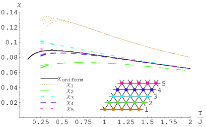
Figure 3: [Color online] The uniform susceptibility and the local susceptibilities at the first five inequivalent neighbors of the boundary. The four curves for each $\chi$ are the Pade approximants [5,6],[5,7],[6,6],[6,7]. $\chi$ is in units of $(g\mu_{B})^{2}/J$.

We see that the ratio of the local susceptibility to the uniform one is somewhat larger for the first neighbor here than in the single vacancy case and more importantly the temperature dependence is stronger. Furthermore, the line impurity is an extended object, so a much larger number of sites is affected. We do not know how common such grain boundaries are in the $\kappa$-(ET)₂Cu₂(CN)₃ material to make predictions for the experiment. However, as in the case with vacancies, we see that down to $T\sim J/4$ only the first few $\chi_{i}$ near the boundary deviate significantly from the bulk value. Thus to explain the experimental lines with such defects we would require a large density of them.

IV Spin Liquid with Fermionic Spinons

The $\kappa$-(ET)₂Cu₂(CN)₃ system does not order down to temperatures as low as $32$ mK, but has a $J\approx 250$ K. Thus it is a good candidate for spin liquid. Among SU(2)-invariant spin liquids constructed using fermionic spinons, the uniform spin liquid has the lowest variational energy in the relevant model with ring exchanges.ringxch It consists of spinons hopping on triangular lattice with no fluxes and thus having Fermi surface. In the full theory, the spinons are coupled to a U(1) gauge field. SSLee ; LeeNagaosaWen ; Ioffe ; LeeNagaosa ; Polchinski ; Altshuler This is hard to solve directly. In order to make progress we solve the problem in the mean field theory ignoring the gauge field and obtaining a system of free fermions hopping on the triangular lattice. We also go beyond mean field by using Gutzwiller projection.

Specifically, in the mean field, we consider free fermions hopping on the triangular lattice in the presence of a missing site, a line boundary, a finite density of missing sites, and also a random distribution of hopping amplitudes. These are models of non-magnetic disorder in terms of what the spinons see.

If $\{\psi_{n}(i)\}$ is the set of single-particle wavefunctions, it is easy to show that the local susceptibility at temperature $T$ is given by

$$\chi(i) = \frac{(g\mu_{B})^{2}}{2T}\sum_{n}|\psi_{n}(i)|^{2}f(\epsilon_{n})(1-f(\epsilon_{n}))~{},$$ (2)

where $f$ is the Fermi function $f(\epsilon)=1/(e^{(\epsilon-\mu)/T}+1)$. In each model of impurities, we obtain the wavefunctions and use this formula to obtain the local susceptibility. We consider various kinds of disorder in turn. We present the results, a very basic discussion, and leave proper discussion of the possible connection to the $\kappa$-(ET)₂Cu₂(CN)₃ to a later section.

Below we keep the spinon hopping $t$ fixed and vary the temperature, and the presented susceptibilities are in units of $(g\mu_{B})^{2}/t$. In a more systematic calculation, the spinon hopping amplitudes would need to be found self-consistently for a given spin Hamiltonian and temperature $T$. In the clean system, the self-consistent $t$ vanishes above some temperature of order $J$ (e.g., in the renormalized mean field scheme this temperature is $0.75J$). When $t$ becomes non-zero, this signals that the system becomes correlated paramagnet, and the spinon mean field is one attempt to capture the growing local correlations. Below the onset temperature, the self-consistent $t$ quickly approaches the zero-temperature value, and it is this regime that we are describing when keeping $t$ fixed. We can estimate the spinon hopping amplitude in the renormalized mean field scheme as $t=3J\langle f_{i}^{\dagger}f_{j}\rangle\approx 0.5J$. The free fermion susceptibility on the half-filled triangular lattice with such $t\sim 100$K would be $\chi\sim 10\cdot 10^{-4}$ emu/mol, which is about a factor of 2-3 larger than the experimental values, but is reasonable given the serious approximations in such calculations.

We further discuss the self-consistent approach in the case with random bond disorder in Sec. IV.4. Before that in the examples below, we introduce the disorder into the spinon problem by hand, either by simply removing the links to vacancy sites, or by taking randomly distributed bonds.

IV.1 Point Impurity

In this case we find the mean field wavefunctions numerically by exact diagonalization for system sizes up to $80\times 80$. The resulting local susceptibility curves for several neighbors of the vacancy are in Figure 4.

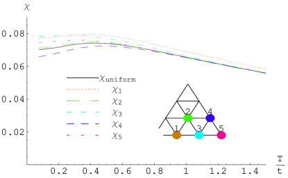
Figure 4: [Color online] The uniform susceptibility and the local susceptibilities at the first five inequivalent neighbors of the impurity obtained for the system of free fermions hopping on the triangular lattice at half-filling. The spinon hopping $t$ is kept fixed and the susceptibilities are in units of $(g\mu_{B})^{2}/t$.

Precise curves for the susceptibility are hard to obtain at low temperatures because of the factor $f(1-f)$ in Eq. (2), which becomes increasingly sharp as $T\to 0$. Thus fewer and fewer states near the chemical potential contribute and eventually the results are polluted by finite size effects. Nevertheless, we can go to sufficiently low temperatures with our system sizes, and the results in Fig. 4 for $T\gtrsim 0.1t$ essentially represent the infinite-volume limit. We see that as we lower the temperature, susceptibilities at more and more neighbors become separated from the uniform susceptibility.

It is interesting to look at the shape of the local susceptibility as a function of the position. At a low temperature ($T=0.054t$) this is plotted in Figure 5 as obtained from the exact lattice calculation.

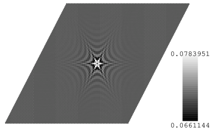
Figure 5: Local susceptibility near impurity at $T=0.074t$ obtained from the free fermion calculation for size $80\times 80$.

This distribution converges to a zero temperature distribution. We can obtain some intuition about the long distance behavior from a calculation treating the non-magnetic impurity as a perturbation. The result is

$$\chi_{\rm loc}(r)-\bar{\chi}=A\frac{\cos(2k_{F}r+\phi)}{r}.$$ (3)

Here $k_{F}$ is the Fermi surface location where the group velocity points in the observation direction $\vec{r}$, while the phase $\phi$ depends on the impurity type and strength (just as in the case of Friedel oscillations in metals). The calculation leading to this result is summarized in Appendix A.

In the present case, the Fermi surface is roughly a circle with $k_{F}\approx[2.67,\;\dots,\;2.72]\,a^{-1}$, where $a$ is the lattice spacing. Taking the above expression and plotting it on the lattice gives a picture looking very similar to Figure 5. One interesting thing to notice is that there is seemingly much longer wavelength along the $\hat{x}$ direction than $\pi/k_{F}$. This simply comes from the fact when we evaluate the $\cos(2k_{F}x+\phi)$ on the lattice, it picks up similar points at different hills of the cosine curve because the period $\pi/k_{F}\approx 1.18a$ is close to one lattice spacing.

At a finite temperature, the oscillatory power law is cut off at the characteristic length

$$\xi(T)=\hbar v_{F}/(2\pi T)~{}.$$ (4)

For the half-filled band on the triangular lattice, the Fermi velocity $v_{F}$ does not vary significantly with the direction and is $v_{F}\approx[2.86,\;\dots,\;2.44]ta/\hbar$. As an example, for $T=0.1t$ the correlation length is only $\xi\approx 4a$.

Finally, we would like to know if this distribution, with one impurity per 10000, can roughly give the observed spectral lines in the $\kappa$-(ET)₂Cu₂(CN)₃ material. The answer is no, and the histograms of $\chi$ are still negligibly narrow.

IV.2 Line Defect

In the clean system with the boundary we can write all wavefunctions explicitly. The resulting susceptibilities are shown in Figure 6 for the first five neighbors as a function of temperature and in Figure 7 for fixed $T=0.0364t$ as a function of the distance from the boundary.

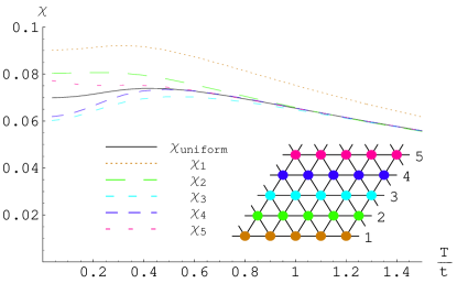
Figure 6: [Color online] The uniform susceptibility and the local susceptibilities at the first five inequivalent neighbors of the boundary obtained for the system of free fermions. $\chi$ is in units of $(g\mu_{B})^{2}/t$.

Figure 7: The local susceptibility as a function of the distance from the boundary $x$ (line index in Fig. 6) at $T=0.0364t$. Note that the vertical scale does not start at zero and that the $x\geq 2$ sites lie withing $\pm 15\%$ window around the average.

Continuum calculation with a circular Fermi surface predicts at $T=0$

$$\frac{\chi_{\rm loc}(r)-\bar{\chi}}{\bar{\chi}}=-J_{0}(2k_{F}r)\approx-\frac{\cos(2k_{F}r-\pi/4)}{\sqrt{\pi k_{F}r}}~{},$$ (5)

where $J_{0}$ is the Bessel function of the first kind and $r$ is the normal distance from the boundary. The asymptotic form is valid also for general Fermi surface, with $k_{F}$ denoting the momentum where the group velocity is perpendicular to the boundary.

A finite temperature cuts off the power at the length scale $\xi(T)$: Roughly, the oscillatory piece is multiplied by $r/[\xi\sinh(r/\xi)]$. Indeed a six-parameter function $a_{0}+a_{1}\cos(a_{2}r-a_{3})/[r^{a_{4}}\sinh(a_{5}r)]$ fits the data like that in Fig. 7 well with $a_{2}\approx 2k_{F}$, $a_{4}\approx-0.5$, and $a_{5}\approx 1/\xi$, in agreement with our expectations. One interesting thing to notice in Fig. 7 is the apparent period of 4 in terms of the lattice line spacing; the wavelength in the continuum $\pi/k_{F}$ is very accurately $4/3$ of the line spacing, so the apparent period is equal to three wavelengths, which is an accidental commensuration effect.

Finally, we look at the histogram of susceptibilities. This depends on the size of the grain – in the present model, the distance between boundaries. To show an example, we consider the system as in Fig. 6 with boundaries separated by 100 lines of sites. The result is in Fig. 8. The grain boundary can in principle go in many directions or might not be straight at all. For the particular orientation that we have chosen, the near commensuration mentioned above plays a role at low temperatures: For our grain size, as we lower $T$, the susceptibilities start to fail to reach the bulk value, and thus we obtain a double peak in the histogram (one peak from the up hills of the sine curve and the other from the down hills, cf. Fig. 7). This starts to happen for temperatures just slightly below the smallest one shown in Fig. 8.

We do not know if this type of disorder is realistic in the $\kappa$-(ET)₂Cu₂(CN)₃. The chosen separation of 100 spacings between boundaries is a rather significant disorder: 2% of the sites are right next to the boundaries and several times more are in the immediate vicinity. Still, at temperature above $0.1t$ the histograms are very narrow ($\xi$ is still smaller than 5 lattice spacings), which is why they are shown only below this temperature. Even at the lowest temperature the linewidth is small, despite the slow decay of $\chi_{\rm loc}(r)$ away from the boundary. Thinking about the $\kappa$-(ET)₂Cu₂(CN)₃, it appears that we need more disorder than this and more spread across the system.

Figure 8: Histogram of the susceptibilities for the system with grain boundaries separated by 100 lines of sites.

IV.3 5% of Impurities

In this section we calculate the susceptibility histogram for the samples with 5% of spin vacancies. It seems unlikely that this type of disorder is present in the $\kappa$-(ET)₂Cu₂(CN)₃in the form of missing ET dimers. However, this could be a crude spin model if the electron charge distribution is inhomogeneous. There are other likely sources of disorder and this case represents a situation when the disorder is point-like. The resulting histograms are in Figure 9. We see that peak is quite broad, more like the experimental curves, and it spreads as we lower the temperature.

Figure 9: Histogram of the susceptibilities for the system with 5% of vacancies. Note especially that the peaks broaden as we lower the temperature. The curves are obtained for $60\times 60$ samples and are in the thermodynamic limit for temperatures shown.

IV.4 Random Spinon Hopping Amplitudes

In this section we take a model of non-magnetic disorder where the spinon hopping amplitudes are random and uniformly distributed in the range $[t-\Delta,t+\Delta]$. The resulting histograms for $\Delta/t=0.2$ are in Figure 10. Note specifically that the peak of the histogram does not change much below roughly $T=0.44t$ (the peak does not spread).

We also tried to make disorder more point-like and see if this would cause the peak to spread, as it did for the point-like missing sites above. We find that this is indeed the case for the following simple choice: Take $95\%$ of bonds to have one value and $5\%$ to have twice as large value (results not shown).

The fact that point-like disorder spreads the peak upon lowering temperature can be understood as follows. As we lower $T$ the correlation length $\xi(T)$ grows and more and more sites start to “feel” the impurities and have susceptibility substantially different from the bulk value. This will be happening until the correlation length becomes somewhat larger than the typical spacing between the point impurities. For the samples studied we can go as low as $T=0.05t$ (before finite size effects set in), and at this $T$ the correlation length is roughly ten lattice spacings. Thus we don’t expect the histogram in Fig. 9 with $5\%$ vacancies to broaden much as the temperature is lowered further.

Figure 10: Histogram of the susceptibilities for the system with random values of bonds with randomness $\pm 20\%$. Note especially that the peaks do not broaden significantly below $T\approx 0.44t$. The curves are obtained for $60\times 60$ samples and are in the thermodynamic limit for temperatures shown.

So far we took a specific fixed distribution of spinon hopping amplitudes and calculated susceptibilities. As we argue below, this is reasonable for a model of non-magnetic disorder where couplings in the spin Hamiltonian have some randomness (assuming it is not too strong and the spin liquid state remains stable). To treat the system more properly, the spinon hopping amplitudes should be calculated self consistently. For example, in the Heisenberg model with exchanges $J_{rr^{\prime}}$, popular mean field self-consistency conditions read $t_{rr^{\prime}}^{*}=\tilde{J}_{rr^{\prime}}\langle f^{\dagger}_{r}f_{r^{\prime}}\rangle$; the bond expectation value is for one spin species and $\tilde{J}_{rr^{\prime}}$ is proportional to $J_{rr^{\prime}}$, e.g., in the so-called renormalized mean field scheme one takes $\tilde{J}=3J$. In the clean system, the above self-consistency condition has non-trivial solution once the temperature is lower than $T=\tilde{J}/4$. Rather quickly below this temperature the spinon hopping becomes large and comparable to the zero-temperature limit. However, in this specific treatment, the spin liquid with the Fermi surface is not a stable solution and other spin liquids perform better. Furthermore, as is known from early slave particle studies, the best states in this mean field are dimerized. In particular, if we try to solve the self-consistency equations by iteration starting from a random initial $t_{rr^{\prime}}$, these run away towards some dimerized solutions.

As discussed in the introduction, we expect that there are additional spin interactions such as ring exchanges that stabilize the zero flux spin liquid against other spin liquid states and dimerized states. Ref. ringxch, presented a schematic mean field argument how the ring exchanges achieve this. The self-consistency condition is modified to

$$t_{rr^{\prime}}^{*} = \tilde{J}_{rr^{\prime}}\langle f^{\dagger}_{r}f_{r^{\prime}}\rangle+\sum_{ss^{\prime}}\tilde{K}_{P}\langle f^{\dagger}_{r}f_{s}\rangle\langle f^{\dagger}_{s}f_{s^{\prime}}\rangle\langle f^{\dagger}_{s^{\prime}}f_{r^{\prime}}\rangle~{},$$ (6)

where $s,s^{\prime}$ are all the sites so that each expectation value is for two sites on a bond, and such sum effectively covers all four-site rhombi $P=[rss^{\prime}r^{\prime}]$ on the triangular lattice that contain the bond $rr^{\prime}$. The couplings $\tilde{K}_{P}$ are proportional to the ring exchanges acting around the rhombi.

Ref. ringxch, applied the above scheme to the clean system at $T=0$ and found that the uniform spin liquid with no fluxes in the hoppings is a stable solution for $\tilde{K}/\tilde{J}>9.9$. Note that the parameters $\tilde{J}$ and $\tilde{K}$ are related to the microscopic Heisenberg and ring exchanges by disparate numerical factors, and Ref. ringxch, contains more details in what sense such $\tilde{K}/\tilde{J}$ values are reasonable in the study of the spin liquid. Here we mainly use this scheme to have a starting point where the uniform state is stable in the clean system and see crudely how the randomness in the microscopic parameters like $J$ translates to randomness in the spinon hopping amplitudes.

To get some understanding of the self-consistent distribution of $t_{rr^{\prime}}$ and its temperature dependence we iterated Eq. (6) until convergence for the following system parameters. We took $\tilde{K}_{P}=15$ everywhere and took a uniformly distributed $\tilde{J}_{rr^{\prime}}$ from the interval $[1-\Delta,1+\Delta]$ for two values $\Delta=0.05,0.2$. We find that once the nontrivial solutions appear, which happens quickly below $T\sim 1/4$ (in units of $\tilde{J}$), the distribution of $t_{rr^{\prime}}$ is essentially independent of the temperature and has the same width in relative terms as the distribution of $\tilde{J}_{rr^{\prime}}$ but is a bit more rounded. Calculating histogram of susceptibilities for this distribution gives roughly the same result as calculating it for the box distribution of $t_{rr^{\prime}}$’s of the same relative width as that of $\tilde{J}_{rr^{\prime}}$. This provides some justification to the preceding models of disorder where we simply put randomness into the spinon problem by hand.

IV.5 Gutzwiller Wavefunction Study of the Local Magnetization

Let us discuss the spin liquid picture beyond the mean field. One way to proceed is to consider effective gauge theory description where spinons interact with the emergent gauge field. One expects that the power laws in Eqs. (3,5) are modified by the gauge field fluctuations,Kolezhuk06 ; Kim03 ; new_power but reliable quantitative information is lacking.

In this work we go beyond the mean field by Gutzwiller projection. In the 1D case, this essentially reproduces exact resultEggert95 for the Heisenberg system with a nonmagnetic impurity. However, in 2D the Gutzwiller projection alone likely does not capture all important fluctuations in the low-energy theory.ringxch Nevertheless, by working directly with the physical spin variables, it gives quantitatively more plausible results than the mean field.

Specifically, we consider local magnetization distribution in a partially polarized state both in the mean field and after the projection. We used this approach to study non-magnetic impurities in a kagome spin liquid in Ref. kagome_w_vacancies, (this reference also contains more discussion on the connection to the local susceptibilities).

It is well known that the Gutzwiller-projected Fermi sea is an excellent trial wavefunction for the 1D spin-1/2 chain, and we test our approach in this case. Figure 11 shows results for a chain with open boundaries. In the mean field, the local magnetization is $\chi_{\rm loc}(x)\sim 1-\cos(2k_{F}x)=1-(-1)^{x}$. The projection dramatically enhances the staggered component. In the Heisenberg chain, Eggert and AffleckEggert95 predict that the staggered component in $\chi_{\rm loc}$ grows as $\sqrt{x}$ away from the boundary at $T=0$, and the Gutzwiller-projected state appears to capture this result in the $m_{\rm loc}$. This dramatic behavior of the $\chi_{\rm loc}$ near a non-magnetic impurity has been used to explain broad lines in spin-1/2 chain compounds even with small density of impurities.1D_experiments

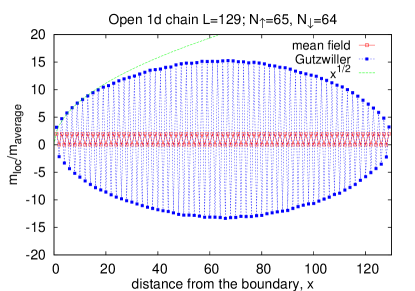
Figure 11: [Color Online] Local magnetization profile in a 1D chain of length $L=129$ with open boundaries before and after Gutzwiller projection of a partially polarized spinon Fermi sea state, here with $N_{\uparrow}=65$, $N_{\downarrow}=64$. The excess up spin occupies orbital $\sin(k_{F}x)=\sin(\pi x/2)$, producing a staggered component in $\chi_{\rm loc}$ with a constant amplitude. The projection dramatically enhances the staggered component, which now grows as $\sqrt{x}$ away from the boundary, in agreement with Ref. Eggert95, for the Heisenberg chain. Such effects can produce broad $\chi_{\rm loc}$ histogram even for small impurity density in the 1D chain. We want to contrast this with the 2D case, where we find only a fixed numerical enhancement.

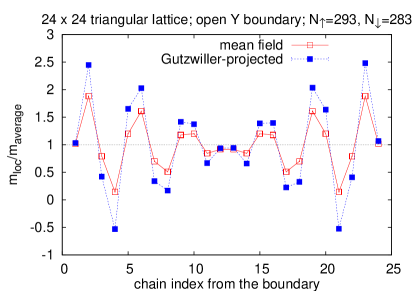
Figure 12: [Color Online] Local magnetization profile in a triangular lattice with grain boundaries before and after Gutzwiller projection of a partially polarized spinon Fermi sea state. The lattice is constructed of 24 chains of length 24, with periodic boundary conditions along the chains and open BC in the perpendicular direction, see the drawing in Fig. 6. The partial spin polarization is obtained starting from an unpolarized state and depopulating 5 spin-down orbitals and occupying 5 spin-up orbitals near the Fermi patch whose normal is perpendicular to the boundary.

Our initial hope was that the 2D spin liquid, which is also a projected Fermi sea state and whose full theory shows enhanced spin correlations at $2k_{F}$, could similarly produce broad $\chi_{\rm loc}$ histograms around small density of impurities. However, it appears that quantitative aspects in 2D are such that small impurity concentration does not give large line broadening.

Specifically, in the 2D spin liquid case, we studied both a single impurity and a line boundary and found that $m_{\rm loc}-\bar{m}$ is enhanced by projection only by a fixed numerical factor of about two. Figure 12 shows representative results in the line boundary case, where the impurity perturbation is the largest of the two cases, cf. Eqs. (3) and (5). The triangular lattice is constructed by stacking 24 chains of length 24, with periodic boundary conditions along the chains and open boundaries in the perpendicular direction. In an effort to bring out more effect, the excess spin-up population occupies orbitals near the patch where the Fermi velocity is normal to the boundaries, since it is this $k$-space region that is responsible for the power law in Eq. (5). Note that because of this special population, the mean field amplitude of oscillations is larger compared to the case with thermal population of orbitals (irrespective of orientation) in Fig. 7. Nevertheless, the figure shows that the Gutzwiller projection gives only a fixed enhancement over the mean field by a factor of about two. Different system sizes and orbital populations do not change this result qualitatively. Similar numerical enhancement was observed in our Kagome study,kagome_w_vacancies where we also argued for it using renormalized mean field thinking.

To conclude, we expect that all our mean field results will experience a similar numerical enhancement in the $\chi_{\rm loc}-\bar{\chi}$ by the projection, so the histograms will be broader by about a factor of two. In particular, we can find negative local susceptibilities, despite the mean field giving only non-negative $\chi_{\rm loc}$. But unlike the 1D, we are not able to get small density of impurities to produce broad lineshapes. One caveat here is that, as we have already mentioned, the Gutzwiller projection in 2D does not capture the full gauge theory, and it could be that the effects of gauge fluctuations are much more dramatic (e.g., see footnote new_power ). This could happen if the actual spin liquid phase has much stronger correlations than the mean field prediction, but at the moment we do not know how to address this better quantitatively.

V Inhomogeneous Knight Shifts in the Metallic Phase

In Sec. IV, we used free fermions as a mean field for the spinons. Assuming the spin liquid is appropriate in the insulator, the treatment further neglects gauge fluctuations and is a crude approximation that can change qualitative long-distance behavior. However, this was best we could do to get some quantitative estimates of local properties.

In fact, the free fermion analysis applies more readily to the metallic phase of the $\kappa$-(ET)₂Cu₂(CN)₃. The fermions are now electrons themselves, and mean field is reasonable in the Fermi liquid regime. We use the same formula Eq. (2) to calculate the local susceptibilities. Also, the analytical results Eq. (3) for the long-distance behavior of $\chi_{\rm loc}(r)$ away from a single impurity and Eq. (5) away from a boundary hold in the metal.

Here we are interested in modelling weak disorder in the metallic phase and connecting with the ¹³C NMR measurements. In this case, we calculate the histogram of susceptibilities in the presence of random on-site potentials taken to be uniformly distributed in an interval $[-W,W]$. The result for $W=0.3t_{e}$ is in Figure 13.

Figure 13: Histogram of the susceptibilities in the metallic phase, where we model disorder by random on-site potentials uniformly distributed in an interval $[-W,W]$ with $W=0.3t_{e}$. The curves are obtained for $60\times 60$ samples and are in the thermodynamic limit for temperatures shown.

Here $t_{e}$ is the electron hopping amplitude and is in excess of 50 meV. This model of disorder is reasonable in the following sense. Note that the disorder strength $W$ should be compared to the band width, which is several times $t_{e}$, so $W=0.3t_{e}$ is a rather weak disorder. A crude Born approximation of the electron mean free path due to elastic scattering in the 2D system gives $k_{F}l\approx\hbar^{2}v_{F}^{2}/(A\overline{\delta\mu^{2}})$, where $A$ is the area per site and $\overline{\delta\mu^{2}}$ is the variance of the on-site potential. For the triangular lattice at half-filling we have $k_{F}l\approx 8t^{2}/\overline{\delta\mu^{2}}$, which gives $k_{F}l\sim 250$ for the above disorder. Direct numerical estimate of the lifetime of momentum eigenstates in the lattice system gives comparable number. Residual resistivities in the $\kappa$-(ET)₂Cu₂(CN)₃ in the metallic phase imply $k_{F}l\gtrsim 50$ and larger, so the disorder that we use is reasonable.

Examining the local susceptibility histograms in Fig. 13, we see that below roughly $T=0.5t_{e}$ the peak no longer spreads. This $T$ is comparable to the room temperature, and indeed the available data in the metallic phase shows little temperature dependence of the linewidth.Kawamoto06 Our model linewidths are reasonable, even though we cannot read off reliably the inhomogeneous broadening component from the lines in Ref. Kawamoto06, .

In the free fermion case of spinons in the previous section we found that making the bond disorder more point-like, by changing value of only a fraction of bonds from the uniform value, the peak of the histogram spreads as we lower the temperature over a wider temperature range compared to the case where some randomness is present on all bonds. In this section we also studied whether similar effect takes place for electrons with random on-site potentials. We set $95\%$ of chemical potentials to zero and $5\%$ to a positive value, chosen to be $0.5t$ in one run and $2t$ in the other. We found that indeed the peaks spread in this case too. This reinforces the conclusion made above that more point-like disorder causes the $\chi_{\rm loc}$ histograms to have stronger temperature dependence of the spread.

VI Discussion

We summarize the main results with an eye to connect with the ¹³C NMR experiments in the $\kappa$-(ET)₂Cu₂(CN)₃.

First, our high-temperature series study shows that the local susceptibility near non-magnetic impurities such as vacancies or grain boundaries can deviate sizably from the bulk value. We studied specifically the Heisenberg model with vacancies and obtained quantitatively accurate results down to $T\sim J/4$. Even at this low temperature, the local susceptibility is modified perceptibly only within few lattice spacings of the defects, cf. Figs. 1 and 3. On the other hand, the ¹³C NMR experiments show broadening that develops gradually from high temperatures; the linewidth roughly doubles going from $T\sim J\sim 250$ K down to $50$ K, at which the FWHM already corresponds to about 20-30% of the bulk susceptibility. In our study, the few close neighbors of the defects show similar deviation in $\chi_{\rm loc}$. However, for a small density of defects, which was our initial assumption, essentially all sites would be sufficiently away from impurities and we would not be able to obtain comparably broad histograms.

We studied vacancies as a model of local nonmagnetic disorder, but we do not expect significant changes for other types of disorder such as random bonds. The Heisenberg model is also not entirely adequate at $T=0$, where multi-spin exchanges likely affect the ground state, but the role of such terms in a nominally spin model is less important at higher temperatures. The Heisenberg model is thus a reasonable choice at such temperatures and was already used successfully to understand the bulk spin susceptibility.Shimizu03 ; Zheng From the high-temperature study with defects, we are led to ask if there is more disorder in the system than originally thought. To be able to reproduce the $T=50$ K lines, we seem to need the disorder strength comparable to that of few percent vacancy concentration. Unfortunately, the way the high-temperature series work, we cannot study directly more realistic models of disorder such as random bonds, but our work with vacancies gives a rough idea.

Next, we considered the spin liquid with spinon Fermi surface as a plausible description of the correlated paramagnet in the temperature range below 50-100 K and down to few Kelvin. This is a serious assumption, and even within it we can do quantitative calculations only in the mean field approximation, supplemented by Gutzwiller renormalizations. Proceeding nevertheless, in such spin liquid at low temperatures, $\chi_{\rm loc}(r)-\bar{\chi}$ decays with slow power laws away from defects, cf. mean field Eqs. (3)new_power and (5), and many sites can be potentially affected by impurities. However, quantitative aspects appear to be such that we would not get visibly broadened histograms even at $T=0$ unless there is a significant density of impurities. If we postulate a sizable disorder, we can get $\chi_{\rm loc}$ histograms comparable to the experimental ones in the temperature range 50 to 10 K. We find that the variation with temperature depends on the type of disorder. If the disorder is uniformly spread, e.g., all bonds are random in some range, the peak stops broadening at a relatively high temperature of about half the overall spinon hopping amplitude. On the other hand, for a more point-like disorder, the peak keeps broadening to much lower temperatures. Thus, if the disorder strength is fixed, in order to get significant temperature dependence of the linewidth in the spinon analysis we would need a point-like disorder.

The free fermion mean field applies directly to the metallic side of the phase diagram of the $\kappa$-(ET)₂Cu₂(CN)₃, which appears for pressures above $0.4$ Gpa. The mean field fermions are now the electrons themselves. What is observedKawamoto06 are essentially temperature-independent ¹³C NMR lines. As a reasonable type of disorder in this case we took a random distribution of the chemical potentials. Specifically, for a box distribution $[-0.3t_{e},0.3t_{e}]$, which gives a reasonably large $k_{F}l\sim 250$, we find sensible and temperature-independent $\chi_{\rm loc}$ histograms. On the other hand, making the disorder more point-like, we find that the histograms broaden as we lower the temperature. Thus on the metallic side the NMR lines suggest a uniformly spread disorder.

Returning to the Mott insulator side, it appears that there is more disorder here than in the same system on the metallic side. Furthermore, if the disorder is fixed as is reasonable in the metal, the metallic side suggests it is uniform and not producing the broadening of the lines, and so this should also be the case on the Mott insulator side, which contradicts the experiments. However, let us assume for a moment that the disorder is point-like. The peak in Fig. 9 produced for $5\%$ vacancies broadens by about a factor of two or three in the range $T=0.5t$ to $0.05t$. Using $t\sim 100$ K, in the experiment this correspond to the range $50$ K to 5 K where we see broadening by about a factor of three which is thus a reasonable agreement. As mentioned, we don’t expect much broadening below $0.05t$ because the correlation length is already about ten lattice spacings which is comparable to the distance between impurities in this example. However the experiment shows very strong broadening beyond that. It might be that the origin of the broadening is not disorder and that our spin liquid picture is not adequate and some other phase is emerging at low temperatures, perhaps with incipient magnetic order.Kolezhuk06 ; Kim03 ; Galitski There is a way to explain the observed phenomena within spin liquid picture, but it seems to require that the disorder strength effectively grows as the temperature is lowered. Below we speculate on how this may come about, but more experimental input is needed.

One source of disorder mentioned in the literature for the (ET)-based organic superconductors is ethylene group disorder.Soto ; Miyagawa This was particularly discussed for the $\kappa$-(ET)₂Cu[N(CN)₂]Br material, where significant sample to sample variations and cooling rate dependence were observed. However, recent studiesWolter ; Maksimuk suggest that the amount of such disorder in the $\kappa$-(ET)₂Cu[N(CN)₂]Br is small at low temperatures and that perhaps the insulating polymeric layer is involved.Wolter

For the spin liquid material $\kappa$-(ET)₂Cu₂(CN)₃, literatureGeiser ; Komatsu ; Kawamoto06 mentions that one of the (CN)^- groups in each unit cell is orientationally disordered and that such structural disorder can generate random electrostatic potential throughout the lattice.Emge If such disorder is indeed involved, the question is then why it does not have comparable pronounced effects on the metallic side. One possible explanation is good screening of charged impurities in the metal and progressively weaker and eventually absent screening in the Mott insulator. For example, in the metallic phase, the Thomas-Fermi screening length is small, $\lambda_{TF}=1/\sqrt{4\pi e^{2}\nu(\epsilon_{F})}\sim 1$ Å, where we estimated the density of states at the Fermi level by $\nu(\epsilon_{F})=0.28/(t_{e}\upsilon)$, $t_{e}=50$ meV is the electron hopping amplitude, and $\upsilon=850.6$ Å³ is the 3D volume per triangular lattice site. On the insulator side, an accurate calculation is harder to make. Using semiconductor language, we can estimate $\lambda=\sqrt{k_{B}T/(4\pi e^{2}n)}$, where $n$ is the number of thermally excited charge carriers. The resistivity of the insulator at ambient pressure increases by about four orders of magnitude when the temperature is decreased from room down to 25 K. Taking this as an order of magnitude measure of the change in the density of carriers, we get $\lambda\sim 10-100$ Å, which is about several lattice spacings. So one scenario is that the charged disorder is still well screened at room temperature but gradually becomes more visible below 100 to 50 K, with the screening essentially absent below about 10 to 5 K. It might be that this type of disorder is more point like, which further enhances the broadening of the $\chi_{\rm loc}$ histogram on the insulator side, but is screened on the metallic side where only weak and more uniformly spread disorder remains that does not cause significant histogram broadening at lower temperatures. In Appendix B, we briefly discuss how the charged disorder in the electronic system may translate to that in the spin model for the insulator.

At present, we do not know how to estimate the strength of disorder in the system and whether the above scenario is reasonable. Unlike the metallic phase, we cannot use the electrical resistivity as a measure of impurity scattering. We want to remark though that if the disorder is not too strong so that the spin-1/2 model with say random couplings is applicable, our spin liquid construction is still a viable candidate for the ground state. As discussed in Sec. IV.4, we can accommodate the bond disorder by adjusting spinon hopping amplitudes, which are now non-uniform. From the point of view of spinons, they are now scattered by this disorder. Interestingly, if the corresponding elastic mean free path is sufficiently small, the thermodynamics of the spinon-gauge system with such diffusive spinons differs from the clean case. Ioffe ; LeeNagaosa For example, the specific heat behaves as $C_{\rm diffusive}\sim T\log(1/T)$ as opposed to the clean system $C_{\rm clean}\sim T^{2/3}$, while the thermal conductivity behaves as $\kappa_{\rm diffusive}\sim T^{1/2}$ as opposed to $\kappa_{\rm clean}\sim T^{1/3}$. The thermal conductivity measurements could potentially give an independent estimate of the degree of disorder in the insulator, while at present the ¹³C NMR is our only window onto the disorder.

Appendix A Perturbative calculation in impurity strength

For a weak non-magnetic perturbation we find, to linear order,

$$\chi_{\rm loc}(q) = \frac{(g\mu_{B})^{2}}{2}u_{\rm imp}\times$$ (7)

$$\times\int_{k} \!\!\!\!\!\!\!\!\!\frac{f(\epsilon_{k})[1-f(\epsilon_{k})]-f(\epsilon_{k+q})[1-f(\epsilon_{k+q})]}{T(\epsilon_{k}-\epsilon_{k+q})}~{},$$ (8)

where $\epsilon(k)$ describes the clean system band structure, while $u_{\rm imp}$ is the appropriate impurity matrix element, for which we neglect any dependence on the momenta. Analyzing the integral in the $T\to 0$ limit, the $q$-dependence has singularities on the $2k_{F}$ surface of the form

$$-\,\frac{\theta(q>2k_{F})}{2\pi v_{F}^{2}\sqrt{c(q-2k_{F})}}~{}.$$ (9)

Here $v_{F}$ is the Fermi velocity and $c$ the curvature at the appropriate Fermi surface patch. Going back to real space, we obtain Eq. (3) with $A=-u_{\rm imp}/(2\pi^{2}v_{F}^{2}c)$ and $\phi=0$.

The $2k_{F}$ oscillations of the local susceptibility of free fermions in the presence of impurities can also be related non-perturbatively to the calculation of the Friedel oscillations in the local density,Kolezhuk06 ; Kim03

$$\rho_{\rm loc}(i) = \sum_{n}|\psi_{n}(i)|^{2}f(\epsilon_{n})~{};$$ (10)

$$\chi_{\rm loc}(i) \sim \frac{\partial\rho_{\rm loc}(i)}{\partial\mu}\sim\frac{\partial\rho_{\rm loc}(i)}{\partial k_{F}}~{}.$$ (11)

This gives one power of $r$ slower decay at large distances in $\chi_{\rm loc}(r)$ than in $\rho_{\rm loc}(r)$ away from defects.

Appendix B From Random Electron Potential to Random Heisenberg J

Here we discuss schematically how disorder in the microscopic electronic model translates to disorder in the effective spin description of the insulator. For an illustration, consider a Hubbard model

$$H=U\sum_{r}n_{r\uparrow}n_{r\downarrow}-\sum_{rr^{\prime}}t_{rr^{\prime}}c_{r\sigma}^{\dagger}c_{r^{\prime}\sigma}+\sum_{r}v_{r}c_{r\sigma}^{\dagger}c_{r\sigma}~{},$$ (12)

with hopping amplitudes $t_{rr^{\prime}}$ and on-site potentials $v_{r}$. Large $U$ opens a charge gap. To leading order in $1/U$, we obtain spin-1/2 model with Heisenberg couplings

$$J_{rr^{\prime}}=\frac{4t_{rr^{\prime}}^{2}}{U\left[1-\frac{(v_{r}-v_{r^{\prime}})^{2}}{U^{2}}\right]}~{}.$$ (13)

Thus, if we have either random hopping amplitudes or random potentials, the Heisenberg couplings are also random.

The randomness in the electron hopping amplitudes translates directly to randomness in the spin exchanges – the latter is even larger in relative terms. On the other hand, if the disorder is in the potentials and if these are much smaller than $U$, this randomness is effectively renormalized down. This is natural since the variables in the spin model are charge-neutral and should be oblivious to such potential disorder. Still, the random potentials are seen via virtual excitations and induce non-magnetic randomness in the spin system.

If we need to include multi-spin exchanges so as to stabilize the spin liquid, there will be some randomness in these as well. Despite the randomness in the effective spin model and irrespective of its electronic origin, as long as it is not too strong, we can proceed with the spin liquid construction but now the spinon hopping amplitudes become non-uniform. This was discussed in Sec. IV.4.

Finally, if the random potentials become comparable to the Hubbard $U$ and lead to significant variation in the electron density, the very spin model thinking can become inappropriate.

References

- (1) Y. Shimizu, K. Miyagawa, K. Kanoda, M. Maesato and G. Saito, Phys. Rev. Lett. 91, 107001 (2003).
- (2) Y. Kurosaki, Y. Shimizu, K. Miyagawa, K. Kanoda, and G. Saito, Phys. Rev. Lett. 95, 177001, (2005).
- (3) A. Kawamoto, Y. Honma, and K. Kumagai, Phys. Rev. B 70, 060510(R) (2004).
- (4) Y. Shimizu, K. Miyagawa, K. Kanoda, M. Maesato, and G. Saito, Phys. Rev. B 73, 140407 (2006); Y. Shimizu, K. Miyagawa, K. Kanoda, M. Maesato, and G. Saito, AIP Conf. Proc. 850, 1087 (2006).
- (5) A. Kawamoto, Y. Honma, K. Kumagai, N. Matsunaga, and K. Nomura, Phys. Rev. B 74, 212508 (2006).
- (6) R. H. McKenzie, Comments Condens. Matter Phys. 18, 309 (1998) (cond-mat/9802198).
- (7) W. LiMing, G. Misguich, P. Sindzingre, and C. Lhuillier, Phys. Rev. B 62, 6372 (2000).
- (8) O. I. Motrunich, Phys. Rev. B 72, 045105 (2005).
- (9) S.-S. Lee and P. A. Lee, Phys. Rev. Lett. 95, 036403 (2005).
- (10) C. P. Nave, S.-S. Lee, and P. A. Lee, Phys. Rev. B 76, 165104 (2007); C. P. Nave and P. A. Lee, ibid. 76, 235124 (2007).
- (11) W. Zheng, R. R. Singh, R. H. McKenzie, and R. Coldea, Phys. Rev. B 71, 134422 (2005).
- (12) F. Wang and A. Vishwanath, Phys. Rev. B 74, 174423 (2006).
- (13) V. Galitski and Y. B. Kim, Phys. Rev. Lett. 99, 266403 (2007).
- (14) Y. Qi and S. Sachdev, arXiv:0711.1538.
- (15) T. Senthil, arXiv:0804.1555.
- (16) S. M. De Soto, C. P. Slichter, A. M. Kini, H. H. Wang, U. Geiser, and J. M. Williams, Phys. Rev. B 52, 10364 (1995).
- (17) K. Miyagawa, A. Kawamoto, and K. Kanoda, Phys. Rev. Lett. 89, 017003 (2002).
- (18) A. U. B. Wolter, R. Feyerherm, E. Dudzik, S. Sullow, Ch. Strack, M. Lang, and D. Schweitzer, Phys. Rev. B 75, 104512 (2007).
- (19) M. Maksimuk, K. Yakushi, H. Taniguchi, K. Kanoda, and A. Kawamoto, Synth. Metals, 149, 13 (2005).
- (20) U. Geiser, H. H. Wang, K. D. Carlson, J. M. Williams, H. A. Charlier, J. E. Heindl, G. A. Yaconi, B. J. Love, M. W. Lathrop, J. E. Schirber, D. L. Overmyer, J. Ren, and M.-H. Whangbo, Inorg. Chem. 30, 2586 (1991).
- (21) T. Komatsu, N. Matsukawa, T. Inoue, and G. Saito, J. Phys. Soc. Jpn. 65, 1340 (1996).
- (22) T. J. Emge, H. H. Wang, M. A. Beno, P. C. W. Leung, M. A. Firestone, H. C. Jenkins, J. D. Cook, J. M. Williams, E. L. Venturini, L. J. Azevedo, J. E. Schirber, Inorg. Chem. 24, 1736 (1985).
- (23) P. A. Lee, N. Nagaosa, and X.-G. Wen, Rev. Mod. Phys. 78, 17 (2006).
- (24) L. B. Ioffe and A. I. Larkin, Phys. Rev. B 39, 8988 (1989). L. B. Ioffe and G. Kotliar, Phys. Rev. B 42, 10348 (1990).
- (25) P. A. Lee and N. Nagaosa, Phys. Rev. B 46, 5621 (1992).
- (26) J. Polchinski, Nucl. Phys. B 422, 617 (1994).
- (27) B. L. Altshuler, L. B. Ioffe, and A. J. Millis Phys. Rev. B 50, 14048 (1994), B. L. Altshuler, L. B. Ioffe, A. I. Larkin, and A. J. Millis, ibid. 52, 4607 (1995).
- (28) T. Itou, A. Oyamada, S. Maegawa, M. Tamura, and R. Kato, J. of Phys. Cond. Mat. 19, 145247 (2007); Phys. Rev. B 77, 104413 (2008).
- (29) J. S. Helton et al., Phys. Rev. Lett. 98, 107204 (2007); O. Ofer et al., arXiv:cond-mat/0610540.
- (30) T. Imai et al., Phys. Rev. Lett. 100, 077203 (2008); A. Olariu et al., Phys. Rev. Lett. 100, 087202 (2008).
- (31) M. A. de Vries et al., Phys. Rev. Lett. 100, 157205 (2008). F. Bert et al., Phys. Rev. B 76, 132411 (2007).
- (32) K. Gregor and O. I. Motrunich, arXiv:0802.0299.
- (33) J. Oitmaa, C. Hamer, and W. Zheng, Series Expansion Methods for Strongly Interacting Lattice Models, (Cambridge University Press, Cambridge, 2006).
- (34) N. Elstner, R. R. Singh, and A. P. Young, Phys. Rev. Lett. 71, 1629 (1993).
- (35) A. Kolezhuk, S. Sachdev, R. R. Biswas, and P. Chen, Phys. Rev. B 74, 165114 (2006).
- (36) Y. B. Kim and A. J. Millis, Phys. Rev. B 67, 085102 (2003)
- (37) Some analytical progress is possible in the case of a single impurity. A separate study sets up self-consistent Eliashberg equations Polchinski ; Altshuler ; Kim03 for the spinon-gauge system in the presence of both the uniform magnetic field and the impurity. The local magnetization is calculated working perturbatively in both the field and the impurity strength. The impurity potential and the local magnetization vertices both become singular at (Ref. Altshuler, ): . The exponent depends on the observation direction if the Fermi surface is not circular (unfortunately we cannot estimate reliably). The power law envelope Eq. (3) is modified to , which could be very slow if is sufficiently large (it may even be increasing away from defects, which would be a dramatic change over the mean field and would resemble the 1D,Eggert95 though this possibility seems less likely in 2D).
- (38) S. Eggert and I. Affleck, Phys. Rev. Lett. 75, 934 (1995).
- (39) M. Takigawa, N. Motoyama, H. Eisaki, and S. Uchida, Phys. Rev. B 55, 14129 (1997); N. Fujiwara, H. Yasuoka, Y. Fujishiro, M. Azuma, and M. Takano Phys. Rev. Lett. 80, 604 (1998).