Discovery of Fast-Moving X-Ray–Emitting Ejecta Knots in the Oxygen-Rich Supernova Remnant Puppis A

Abstract

We report on the discovery of fast-moving X-ray–emitting ejecta knots in the Galactic Oxygen-rich supernova remnant Puppis A from XMM-Newton observations. We find an X-ray knotty feature positionally coincident with an O-rich fast-moving optical filament with blue-shifted line emission located in the northeast of Puppis A. We extract spectra from northern and southern regions of the feature. Applying a one-component non-equilibrium ionization model for the two spectra, we find high metal abundances relative to the solar values in both spectra. This fact clearly shows that the feature originates from metal-rich ejecta. In addition, we find that line emission in the two regions is blue-shifted. The Doppler velocities derived in the two regions are different with each other, suggesting that the knotty feature consists of two knots that are close to each other along the line of sight. Since fast-moving O-rich optical knots/filaments are believed to be recoiled metal-rich ejecta, expelled to the opposite direction against the high-velocity central compact object, we propose that the ejecta knots disclosed here are also part of the recoiled material.

1 Introduction

Puppis A is categorized as an “oxygen-rich” supernova remnant (SNR) based on optical spectroscopy (Winkler & Kirshner 1985). The group of O-rich remnants contains only two other members in our Galaxy, Cassiopeia A (Chevalier & Kirshner 1979) and G292.0+1.8 (Goss et al. 1979), and a few in the Magellanic Clouds (Blair et al. 2000 and references there in). At optical wavelengths, these SNRs show fast-moving metal-rich ejecta knots ($v>1000\,\mathrm{km\,sec^{-1}}$) which are typically enriched in O and Ne. High-Z elements, like Ar, Ca, and Fe, are dominantly generated in a Type-Ia supernova (Nomoto et al. 1984), while low-Z elements, like O, Ne, and Mg, are found in core-collapse SN debris (Thielemann et al. 1996). These facts suggest that O-rich SNRs are core-collapse origin. The detection of metal-rich ejecta from these SNRs thus provides us with an opportunity to make a direct test of core-collapse SN nucleosynthesis models.

O-rich fast-moving optical knots (hereafter, OFMKs) in Puppis A, whose proper motions are all consistent with undecerelated expansion from a common center (Winkler & Kirshner 1985; Winkler et al. 1988), have been found only in the northeastern quadrant, suggesting asymmetric mass ejection during SN explosion which produced Puppis A. On the other hand, proper motion of a central compact object (CCO), RX J0822-4300, associated with the Puppis A SNR was recently measured to be directed toward the southwest with a high velocity of $\sim$1600 km sec^-1 (Winkler & Petre 2007). The CCO is considered to be kicked by asymmetric mass ejection during the SN explosion according to momentum conservation, from which we can study SN explosion mechanisms (e.g., Scheck et al. 2006).

The so-called “omega” filament (Winkler & Kirshner 1985) is one of the best studied OFMKs in Puppis A. Winkler & Kirshner (1985) observed the “omega” filament and found that the spectrum was dominated by O lines, with rather weak Balmer lines. The mass ratio of O to H was estimated to be 30, i.e., $\sim$2000 times the solar value. Furthermore, they found that the O lines were blue-shifted by 1500$\pm 100$ km sec^-1. These facts led them to consider that the “omega” filament was nearly pure O ejecta from the core of the SN progenitor that had remained more or less intact.

In X-ray wavelengths, Puppis A generally showed sub-solar metal abundances, suggesting that the X-ray emission from Puppis A was dominated by the swept-up interstellar medium (Tamura 1995; Hwang et al. 2008). The complex interstellar environment such as a gradient in the ambient density (Petre et al. 1982) as well as the relatively old age of $\sim$4000 years (Blair et al. 2003) might have made it difficult to detect clear signs of metal-rich ejecta in its spectra. However, recent Suzaku observations revealed metal-rich ejecta features in the northeastern part of the remnant (Hwang et al. 2008). Here, we also report of the discovery of the X-ray–emitting fast-moving ejecta knots positionally coincident with the optical “omega” filament.

2 Observations and Data Reduction

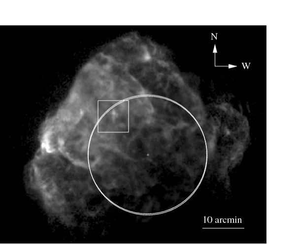
Figure 1: XMM-Newton FOV (white circles) overlaid on a ROSAT HRI image of the entire Puppis A SNR. The data have been smoothed by Gaussian kernel of $\sigma=15^{\prime\prime}$. The intensity scale is square root. Optical O III and XMM-Newton three-color images in the white box region are shown in Fig. 2.

Parts of Puppis A have been observed several times with XMM-Newton. Among them, two observations (ObsIDs. 0113020101 and 0113020301) cover the “omega” filament (Winkler & Kirshner 1985). The fields of view (FOV) of the two XMM-Newton observations are shown on a ROSAT HRI image of the entire Puppis A in Fig. 1. All the raw data were processed with version 6.5.0 of the XMM Science Analysis Software. We use only MOS data, since the pn data were obtained in PrimeSmallWindow mode so that the pn FOV covered only a small region around the CCO that is not focused in this paper. We select X-ray events corresponding to patterns 0–12. We further clean the data by rejecting high background (BG) intervals and remove all the events in bad columns listed in Kirsch (2006). The summed exposures from the good time intervals (GTIs) after data cleaning are 22 ks for ObsID. 0113020101 and 10.8 ks for ObsID. 0113020301, respectively. After the filtering, the data were vignetting-corrected using the sas task evigweight.

3 Analysis and Results

Fig. 2 Left shows the optical O III image. We can see an $\Omega$-shaped filament, so-called “omega” filament in the central portion of the figure. Fig. 2 Right shows an X-ray three-color image of the merged MOS1/2 data which covers the same area. Red, green, and blue represent 0.4–0.7 (for O lines), 0.7–1.2 (for Ne lines), and 1.2–5.0 (for hard band) keV, respectively. We find an X-ray–emitting knotty feature in the central portion of Fig. 2 Right. The southern region of the feature is positionally coincident with the optical “omega” filament as indicated by box regions in Fig. 2.

We extract spectra from the north and south of the X-ray knotty feature because it is divided into two regions in terms of color: the NE region of the feature shows white color indicating a significant mixture of spectrally hard emission, while the SW region of the feature shows soft red emission. The two regions are shown as a white solid circle (radius of 30^′′) and a white solid ellipse (angular sizes of x and y-axis of 20^′′ and 40^′′, respectively) in Fig. 2 Right. Note that the southern region in the feature includes the “omega” filament. We simultaneously fit the MOS1 and MOS2 spectra, allowing the normalizations between the two detectors to vary by introducing the constant model in XSPEC (Arnaud 1996). As BG, we subtract the X-ray emission in their surrounding regions (i.e., areas enclosed by dashed lines around each region shown in Fig. 2 Right) after normalizing the intensities at the ratios of source areas to BG areas. In this way, we attempt to obtain the spectra of the knotty feature itself. We note that our method is not unprecedented; the same method was successfully performed in analyses of ejecta knots in Cas A SNR (Hwang & Laming 2003; Laming & Hwang 2003). The count rates per area of the source and BG regions are summarized in Table 1.

We apply an absorbed single component non-equilibrium ionization (NEI) model for the two spectra (the wabs (Morrison & McCammon 1983) and vpshock model (NEI version 2.0) (e.g., Borkowski et al. 2001) in XSPEC v 12.3.1). Initially, we allow the individual element abundances to be freely fitted relative to H and find that enhanced values are required. This fact clearly shows that the knotty feature consists of metal-rich ejecta. The northern region is rich in O, Ne, Mg, Si, S, and Fe, whereas the southern region is rich in O, Ne, and Mg. We note that Hwang et al. (2008) independently detect metal-abundance enhancements positionally coincident with the X-ray knotty feature disclosed here from their Suzaku observations, although the relatively low spatial resolving power of Suzaku prevented them from identifying the metal-abundance enhancements with the “omega” filament. We then set O/H at the optically determined value of 2000 (Winkler & Kirshner 1985) in order to obtain element abundances relative to O. Free parameters are hydrogen column density, $N_{\mathrm{H}}$; electron temperature, $kT_{\mathrm{e}}$; ionization timescale, $n_{\rm e}t$; volume emission measure (VEM; VEM $=\int n_{\mathrm{e}}n_{\mathrm{H}}dV$, where $n_{\mathrm{e}}$ and $n_{\mathrm{H}}$ are number densities of electrons and protons, respectively and $V$ is the X-ray–emitting volume); abundances of Ne, Mg, Si, S, Fe, and Ni. Above, $n_{\rm e}t$ is the electron density times the elapsed time after shock heating and the vpshock model assumes a range of $n_{\rm e}t$ from zero up to a fitted maximum value. We set the abundance of Ni equal to that of Fe. Abundances of the other elements are fixed to the solar values Anders & Grevesse (1989).

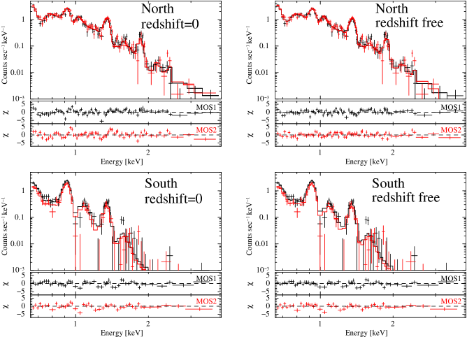
Figure 3: Left column: MOS1 (black) and MOS2 (red) spectra from the two regions in Fig. 2 with the best-fit model (redshift = 0). The lower panels show the residuals. Right column: Same as the left column but with the revised model (redshift is free).

The two spectra, along with the best-fit models, are shown in Fig. 3 (left column). Note that we exclude data in the energy range below 0.65 keV where apparent differences between MOS1 and MOS2 data are seen. The difference might be due to the contamination on the MOS1 chip (Pradas & Kerp 2005). The best-fit parameters and fit statistics are summarized in Table 2. We find that the fit level for the northern spectrum is far from acceptable while that for the southern one is moderate. We notice that the residuals in the northern spectrum have wavy structures around several lines such as Ne He$\alpha$, Mg He$\alpha$, or Si He$\alpha$. These features suggest that the line center energies are systematically shifted from those expected by the best-fit model.

We thus introduce a variable redshift in the same vpshock model. The two spectra with the revised best-fit model are also shown in Fig. 3 (right column). The revised model significantly improves the fits for both of the two spectra (with a significance level of greater than 99.9% based on the $F$-test). In particular, the wavy structures of residuals seen in the previous fit, where the redshift is fixed to zero, for the northern spectrum are greatly reduced in the revised fit, where the redshift is free. Table 2 summarizes the best-fit parameters for the two spectra obtained from the revised model fitting. The derived redshift parameter shows negative, i.e., blue-shifted values in the two regions. The value of the blueshift for the northern region of the X-ray knotty feature is higher than that for the southern region. We find that a relatively low temperature and little evidence of Si and S abundances in south of the feature, while relatively high temperatures and significant Si and S abundances in the north of the feature. Those facts result in the color variation seen Fig. 2 Right. Ionization timescales for the two regions are significantly lower than that expected for the collisional ionization equilibrium.

Doppler velocity measurements with X-ray CCD detectors have been successfully demonstrated by several different groups (e.g., Willingale et al. (2002) using data from XMM-Newton MOS). However, small redshifts of $\lesssim 10$ eV require careful investigation of systematic uncertainties and/or artifacts due to the detector calibration (the uncertainty of absolute energy scale is $\lesssim$ 5 eV; Kirsch 2007). To estimate systematic errors of the derived Doppler shifts, as well as to ensure that the line shifts are not due to calibration uncertainties, we further perform spectral analysis in the following three cases: (1) individual fit of MOS1 and MOS2 spectra, (2) individual fit of spectra from the two observations (whose rotation angles are different from each other), (3) inhomogeneous intensities of BG spectra, in case that the intensities of the BG spectra in the source regions are different from those in the BG regions currently selected. We examine 50% higher or lower than the original intensity since there are inhomogeneities of X-ray intensities of $\sim$50% around the X-ray knotty feature. We summarize all the derived values of the redshift in Table 3. We find significant blueshifts in all the cases for the two regions. The systematic uncertainties are greater than the statistical ones and dominate the significance of the redshift. The Doppler velocities, considering all the systematic uncertainties, are $-3400^{+1000}_{-800}$ km sec^-1 for the north of the X-ray knotty feature and $-1700^{+700}_{-800}$ km sec^-1 for the south of the feature. The dominant uncertainty comes from the systematic uncertainty between the two detectors and/or that introduced by possible variations of the BG intensities. We should note that the values of metal abundances vary by factors of $\sim$3 in the three cases of BG intensities examined. This systematic uncertainty is considered to be conservative errors of the abundances obtained.

Next, we investigate whether or not the calibration uncertainty of the MOS energy scale is serious in our data. We measure line center energies in the two regions and the local BG region for each region, applying a phenomenological model, i.e., a thermal continuum and 14 Gaussian line profiles. The center energy, line width, normalization of each Gaussian line, as well as the temperature and normalization of the thermal continuum, were treated as free parameters. The derived line center energies for Ne He$\alpha$, Mg He$\alpha$, and Si He$\alpha$ are summarized in Table 4. We confirm that the line center energies obtained in the local-BG-subtracted spectra are indeed significantly higher than those obtained in the surrounding BG regions. Furthermore, the blueshifts implied by simply comparing the source and BG line centers are quite similar to that found in the NEI best-fit models. These facts strongly support the suggestion that the line shifts seen in the ejecta feature are not due to calibration uncertainties of the MOS energy scale.

Finally, we investigate whether the variations of line center energies are caused by the plasma condition (i.e., ionization states, electron temperature) rather than Doppler shifts. According to the NEI code in Hughes et al. (2003), line center energies of the K-shell complex, including all lines from all charge states excluding Ly$\alpha$ and all higher energy lines are calculated to be 0.872–0.918 keV for Ne, 1.269–1.350 keV for Mg, and 1.744–1.862 keV for Si. The results in Table 4 show that the shifts in line centroids from the northern region cannot be related to temperature/ionization effects, while the effects cannot be ruled out for the south region. However, the agreement with optical Doppler velocity makes it plausible that we detect blueshift in the south region.

In this context, we are convinced that the line shifts observed in the two regions are due to neither instrumental origin nor plasma conditions (i.e., $kT_{\mathrm{e}}$ and $n_{\rm e}t$) but reflect the Doppler-shifts caused by their fast motion toward us. In conclusion, we observe blue-shifted line emission from the north and south of the X-ray knotty feature with Doppler velocities of $-3400^{+1000}_{-800}$ km sec^-1 and $-1700^{+700}_{-800}$ km sec^-1, respectively. The Doppler velocity estimated in the south of the X-ray knotty feature, where the optical “omega” filament is included, is consistent with that measured for the optical “omega” filament (1500$\pm$100 km sec^-1; Winkler & Kirshner 1985).

4 Discussion

We find an ejecta-dominated X-ray bright knotty feature on the position of the optically O-rich filament discovered by Winkler & Kirshner (1985) and Winkler et al. (1988). Due to its fast motion toward us, we detect blue-shifted lines from the feature. The Doppler velocity in the northern region of the feature is higher than that in the southern region. If they are moving with different velocities, distances from the explosion center are also different with each other. This means that we see two different ejecta knots that are close to each other along the line of sight. Follow-up work with data of better spatial resolution (i.e., Chandra data) might reveal clear morphological separation between the north knot and south knot.

4.1 Mass and Origin of the Fast-Moving Ejecta Knots

Under the assumption of metal abundance of O/H to be 2000 times the solar value, the electrons are dominantly supplied by O or other metals such as Si or S. We assume that the value of $n_{\mathrm{e}}$ is 7 times that of the O ion density, $n_{\mathrm{O}}$, because O ions mainly exist in the He-like or H-like ionization states at the electron temperature and the ionization timescale obtained for the knots (Table 2). Assuming that the depth of the X-ray–emitting plasma is the same as the physical scale corresponding to the apparent angular size of the knots (1^′) at a distance of 2.2 kpc (Reynoso et al. 1995), we estimate elemental densities and masses in each region; these are summarized in Table 5. We obtain the total masses in the northern and southern knots to be $\sim$0.07 M_⊙, $\sim$0.08 M_⊙, respectively.

The masses of individual OFMKs seen in Cas A and Puppis A are estimated to be 1$\times 10^{-4}$ M_⊙ (Raymond 1984) and 1$\times 10^{-2}$ M_⊙ (Winkler et al. 1988), respectively. The masses of Fe-rich knots in Cas A and O and Ne-rich knot in G292.0+1.8 are estimated to be 4$\times 10^{-5}$–1$\times 10^{-3}$ M_⊙ (Hwang & Laming 2003) and 1$\times 10^{-3}$ M_⊙ (Park et al. 2004), respectively. The masses of Vela shrapnels A (Si-rich knot) and D (O, Ne, and Mg-rich knot) are estimated to be 5$\times 10^{-3}$ and 0.1 M_⊙, respectively (Katsuda & Tsunemi 2006; Katsuda & Tsunemi 2005). Therefore, the ejecta knots disclosed here are categorized as the most massive ejecta knots.

We investigate the origin of these ejecta material by comparing the observed metal abundance ratios with those of theoretical models. We employed models for various progenitor masses with initial composition of solar values. We examine two sets of models by Rauscher et al. (2002) and Tominaga et al. (2007). For the southern knot, we compare the relative abundances of Ne and Mg to O with those expected in the models, and find that some models by both of the two groups can reproduce the derived relative abundances in the explosive Ne/C-burning cores. On the other hand, the composition of the northern knot turns out not to be reproduced in any models at any mass radius. If we compare the mass ratios of S and Fe to Si to those of the models, we find that all the models examined can reproduce the mass ratios in incomplete explosive Si-burning layers. The progenitor mass and specific burning process are not well constrained by the current data analysis. This is partly because the local BG subtraction affects the abundance determination by a factor of $\sim$3, and partly because emission from north and south knots are contaminating with each other in our current data. Follow-up observations with better spatial resolution are needed to reveal the origins of the two knots as well as the progenitor mass.

4.2 Recoil to the High-Velocity CCO

Considering that OFMKs in Puppis A are believed to be recoiled materials to the high-velocity CCO (Hui & Becker 2006; Winkler & Petre 2007), we suggest that the ejecta knots which we find near the OFMKs are also part of the recoiled materials. Winkler & Petre (2007) measured the proper motion of the stellar remnant and estimated the momentum to be $\sim 4\times 10^{41}\mathrm{g\,cm\,s^{-1}}$ in the plane of the sky. They also estimated approximate total momentum for the 11 measured OFMKs toward the opposite direction to the traveling direction of the CCO to be $\sim 1.3\times 10^{41}\mathrm{g\,cm\,s^{-1}}$, comprising about $\sim$30% of the required momentum to balance that of the CCO. We estimate that for the X-ray–emitting ejecta knots to be $\sim 0.5\times 10^{41}\mathrm{g\,cm\,s^{-1}}$, comprising about 10% of the required momentum. The rest of the required momentum might be explained by unidentified $\sim$20 OFMKs whose existence was suggested in O III image of this remnant (Winkler & Petre 2007).

There are mainly three mechanisms proposed to explain the origin of high-velocity neutron stars such as the CCO in Puppis A: binary disruptions, natal or postnatal kicks from the SN explosions (see, Lai et al. 2001 for a review). Recent theoretical studies have focused on natal kicks imparted to neutron stars at birth rather than the other two mechanisms. A natal kick could be due to global hydrodynamical perturbations in the SN core (e.g., Goldreich et al. 1996), or it could be a result from asymmetric neutrino emission in the presence of super strong magnetic fields ($B\gtrapprox 10^{15}$ G) in the proto–neutron star (e.g., Blandford et al. 1983). The two models lead to distinct predictions: the measured neutron star velocity should be directed opposite to the momentum of the gaseous SN ejecta caused by linear momentum conservation in the hydrodynamically-driven mechanisms (e.g., Scheck et al. 2006) while neutrino-driven mechanisms predict the motion of the ejecta roughly in the same direction of the neutron star kick (Fryer & Kusenko 2006). Therefore, our data as well as the distributions of OFMKs suggest that the hydrodynamically- (or ejecta-)driven mechanisms are at work to produce the high-velocity CCO in Puppis A. However, we should care about the possibility that the lack of OFMKs in the southwestern portion of the remnant might otherwise be explained by complicated structures of the ambient medium (e.g., Petre et al. 1982). Also, the existence of ejecta knots disclosed here is not inherently convincing evidence for a lack of undetected ejecta in other directions, although diffuse X-ray emission is generally reported to have low metal-abundances (Tamura 1995; Hwang et al. 2008). To obtain further conclusive evidence that the ejecta-driven mechanism is at work, we need detailed spatially resolved spectral analysis for the entire remnant.

5 Summary

We have analyzed archival XMM-Newton data of the Puppis A SNR. We disclose an X-ray knotty feature on the position of one of OFMKs discovered by Winkler & Kirshner (1985) and Winkler et al. (1988). We find that the X-ray knotty feature is metal-rich ejecta with blue-shifted emission lines. The composition in the northern region of the feature is different from that in the southern region: O, Ne, Mg, Si, S, Fe-rich in the northern region, whereas O, Ne, and Mg-rich in the southern region. Also, the Doppler velocity in the northern region, $-3400^{+1000}_{-800}$ km sec^-1, is different from that in the southern region, $-1700^{+700}_{-800}$ km sec^-1. These facts lead us to consider that the feature consists of two different knots that are close to each other along the line of sight. Current data are not sufficient to constrain the origins of the two knots as well as to precisely determine the Doppler velocities in the two knots. Further observations with better spatial resolution and better observational condition, especially considering that the knots are located at the edge of FOV in the current data, are strongly required to reveal possible morphological separation between the north knot and south knot, and to accurately determine the compositions as well as Doppler velocities in the two knots.

Table 1: Count rates per area (counts sec^-1 arcmin^-2) in the source and BG regions.

	North	North (BG)	South	South (BG)
MOS1	2.53$\pm$0.01	1.40$\pm$0.01	1.51$\pm$0.01	0.99$\pm$0.01
MOS2	2.42$\pm$0.01	1.26$\pm$0.01	1.37$\pm$0.01	0.99$\pm$0.01

Note. — Count rates are estimated in the energy range of 0.65–4.0 keV.

Table 2: Spectral-fit parameters in the two regions shown in Fig. 2 Right

Region	$N_{\mathrm{H}}$	$kT_{\mathrm{e}}$ (keV)	log($n_{\rm e}t$)	Ne/O	Mg/O	Si/O	S/O	Fe/O	VEMa	redshift ($\times 10^{-3}$)	$\chi^{2}/d.o.f.$
North	0.37${}^{+0.03}_{-0.02}$	1.36${}^{+0.11}_{-0.08}$	10.65${}^{+0.05}_{-0.05}$	0.8$\pm 0.1$	0.8$\pm 0.1$	0.5$\pm 0.1$	0.4$\pm 0.3$	0.22${}^{+0.08}_{-0.06}$	$1.2\pm 0.2$	—	462/216
South	0.43$\pm 0.02$	0.36$\pm 0.02$	10.59${}^{+0.06}_{-0.08}$	1.4${}^{+0.3}_{-0.1}$	1.7${}^{+0.5}_{-0.3}$	$<$1.1	$<$0.7	$<$0.03	2.7$\pm 0.3$	—	290/191
North	0.40${}^{+0.03}_{-0.06}$	0.60${}^{+0.08}_{-0.05}$	11.20${}^{+0.07}_{-0.06}$	1.04${}^{+0.05}_{-0.06}$	0.95${}^{+0.19}_{-0.05}$	0.7$\pm 0.1$	$<$0.8	0.16$\pm 0.03$	$2.2\pm 0.1$	$-11.4^{+0.4}_{-0.3}$	288/215
South	0.43${}^{+0.01}_{-0.02}$	0.35$\pm 0.01$	10.71${}^{+0.02}_{-0.14}$	1.5$\pm 0.1$	1.7${}^{+0.2}_{-0.3}$	$<$0.5	$<$0.7	$<$0.03	2.5$\pm 0.3$	$-5.5^{+0.1}_{-1.0}$	266/190

Note. — The best-fit parameters for the two spectra in Fig. 2 Right. Results are from the vpshock model in which the redshift is fixed to zero (upper two rows) and allowed to vary (lower two rows). The units of $N_{\rm H}$ and VEM are $\times 10^{22}$ cm^-2 and $\times 10^{53}$ cm^-3, respectively. VEM is calculated at a distance of 2.2 kpc (Reynoso et al. 1995). Quoted errors are at 90% confidence level. The values of the abundance ratios are relative to those of the solar ratios. Other elements are fixed to those of the solar values Anders & Grevesse (1989). The errors are calculated after fixing the $kT_{\mathrm{e}}$ to the best-fit value. Errors for VEM are calculated after fixing the $kT_{\mathrm{e}}$ and Ne abundance to the best-fit values.

Table 3: Redshift values ($\times 10^{-3}$)

Region	Case-1a		Case-2b		Case-3c
	MOS1	MOS2	Obs1	Obs2	0.5	1d	1.5
North	$-8.6^{+0.2}_{-0.7}$	$-12.4^{+0.6}_{-0.4}$	$-8.6\pm 0.4$	$-12.6^{+0.7}_{-0.5}$	$-9.0^{+0.2}_{-0.1}$	$-11.4^{+0.4}_{-0.3}$	$-13.9^{+0.1}_{-0.2}$
South	$-5.6^{+1.6}_{-0.9}$	$-5.6^{+2.2}_{-2.8}$	$-5.1\pm 0.2$	$-6.7^{+3.5}_{-1.7}$	$-5.7^{+0.1}_{-0.9}$	$-5.5^{+0.1}_{-1.0}$	$-5.5^{+2.3}_{-1.2}$

Table 4: Line center energies of spectra from regions shown in Fig. 2 Right.

line	North	North (BG)	South	South (BG)
Ne He$\alpha$ (eV)	930${}^{+6}_{-5}$	917$\pm$2	922${}^{+5}_{-3}$	917$\pm$1
Mg He$\alpha$ (eV)	1357$\pm$2	1344${}^{+1}_{-2}$	1351${}^{+3}_{-5}$	1346${}^{+1}_{-3}$
Si He$\alpha$ (eV)	1878${}^{+5}_{-8}$	1856${}^{+4}_{-3}$	NDa	1857${}^{+3}_{-2}$

Note. — Quoted errors are at 90% confidence level. ^aCase-1; we individually analyze MOS1 and MOS2 data. In this case, we include both of the two observations and subtract the local BG with original intensity. ^bCase-2; we separately analyze the data from the two observations. Obs1 and Obs2 are ObsID. 0113020101 and ObsID. 0113020301, respectively. In this case, we use data from both MOS1 and MOS2 detectors and subtract the local BGs with original intensities. ^cCase-3; we artificially vary the intensities of the local BGs (0.5 and 1.5 times the original intensity). In this case, we use all the data sets (MOS1+MOS2+Obs1+Obs2). ^dSame as listed in Table 2.

Note. — Quoted errors are at 90% confidence level. ^aWe could not determined the value due to the poor statistics.

Table 5: Densities (cm^-3) and masses (M_⊙) in the two regions in Fig. 2 Right

	$n_{\mathrm{e}}$	$n_{\mathrm{O}}$	$n_{\mathrm{Ne}}$	$n_{\mathrm{Mg}}$	$n_{\mathrm{Si}}$	$n_{\mathrm{S}}$	$n_{\mathrm{Fe}}$	MO	MNe	MMg	MSi	MS	MFe
North	5	0.7	0.1	0.03	0.02	0.005	0.002	0.05	0.01	0.003	0.003	0.001	0.0015
South	5	0.7	0.15	0.05	0	0	0	0.06	0.015	0.007	0	0	0

Note. — Typical errors (which mainly come from the assumptions of the plasma depth and the filling factor ) are about a factor of 2.

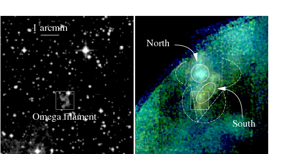
Figure 2: Left: Linearly-scaled Optical O III image for the box region in Fig. 1. The central $\Omega$-shaped filament enclosed in a box region is a so-called “omega” filament (Winkler & Kirshner 1985). Right: XMM-Newton three-color image in the same area. Red, green, and blue represent 0.4–0.7, 0.7–1.2, and 1.2-5.0 keV, respectively. The intensity scale is square root. Spectral extraction regions are shown as solid (for source spectra) and dashed (for BG spectra) white lines. The location of the “omega” filament is indicated as a box region that is the same box in Fig. 2 Left.

References

- Anders & Grevesse (1989) Anders, E., & Grevesse, N. 1989, Acta, 53, 197
- Arnaud (1996) Arnaud, K. A. 1996, ASP Conf. Ser., 101, 17
- Blair et al. (2000) Blair, W. P., Morse, J. A., Raymond, J. C., Kirshner, R. P., Hughes, J. P., Dopita, M. A., Sutherland, R. S., Long, K. S., & Winkler, P. F. 2000, ApJ, 537, 667
- Blair et al. (2003) Blair, W. P., Sankrit, R., Ghavamian, P., Raymond, J. C., and Morse, J. A. 2003, AAS, 203, 3912B
- Blandford (1983) Blandford, R. D., Applegate, J. H., & Hernquist, J. 1983, MNRAS, 204, 1025
- Borkowski et al. (2001) Borkowski, K. J., Lyerly W. J., & Reynolds, S. P. 2001, ApJ, 548, 820
- Chevarier (1979) Chevarier, R., & Kirshner, R. 1979, ApJ, 233, 154
- Fryer (2006) Fryer C. L. & Kusenko, A. 2006, ApJ, 163, 335
- Goldreich (1996) Goldreich, P., Lai, D., & Sahrling, M., 1996, in Unresolved Problems in Astrophysics, ed. J. N. Bahcall, & J. P. Ostriker (Princeston; Princeton Univ. Press), 269
- Goss (1979) Goss, W. M., Shaver, P. A., Zealey, W. J., Murdin, P., and Clark, D. H. 1979, MNRAS, 188, 357
- Hughes (2003) Hughes, J. P., Rakowski, C. E., Decourcelle, A. 2003, ApJ, 543, L61
- Hui (2006) Hui, C. Y., & Becker, W. 2006, A&A, 457, L33
- Hwang (2003) Hwang, U., & Laming, J. M. 2003, ApJ, 597, 362
- Hwang et al. (2008) Hwang, U., Petre, R., & Flanagan, K. A. 2008, ApJ, in press
- Katsuda (2005) Katsuda, S., & Tsunemi, H. 2005, PASJ, 57, 620
- Katsuda (2006) Katsuda, S., & Tsunemi, H. 2006, ApJ, 642, 917
- Kirsch (2006) Kirsch, M. 2006, XMM-EPIC status of calibration and data analysis, XMM-SOC-CAL-TN-0018, issue 2.5
- Kirsch (2007) Kirsch, M. 2007, XMM-EPIC status of calibration and data analysis, XMM-SOC-CAL-TN-0018, issue 2.6
- Lai (2001) Lai, D., Chernoff, D. F., & Cordes, J. M. 2001, ApJ, 549, 1111
- Laming (2003) Laming, J. M., & Hwang, U., 2003, ApJ, 597, 347
- Morrison (1983) Morrison, R., & McCammon, D. 1983, ApJ, 270, 119
- Nomoto (1984) Nomoto, K., Thielemann, F.-K., & Yokoi, K. 1984, ApJ, 286, 644
- Park (2004) Park, S., Hughes, J. P., Slane, P. O., Burrows, D. N., Roming, P. W. A., Nousek, J. A., and Garmire, G. P. 2004, ApJ, 602, L33
- Petre (1982) Petre, R., Kriss, G., A., Winkler, P. F., & Canizares, C. R. 1982, ApJ, 258, 22
- Pradas (2005) Pradas, J. & Kerp, J. 2005, A&A, 443, 721
- Reynoso (1995) Reynoso, E. M., Dubner, G. M., Goss, W. M. & Arnal, E. M. 1995, AJ, 110, 318
- Scheck (2006) Scheck, L., Kifonidis, K., Janka, H.-Th., & Muller, E. 2006, A&A, 457, 963
- Tamura (1995) Tamura, K. 1995 Ph.D. thesis, Osaka Univ.
- Thielemann (1996) Thielemann, F.-K., Nomoto, K., & Hashimoto, M. 1996, ApJ, 460, 408
- Tominaga et al. (2007) Tominaga, N., Umeda, H., Nomoto, K. in prep.
- Willingale et al. (2002) Willingale, R., Bleeker, J. A. M., van der Heyden, K. J., Kaastra, J. S., and Vink, J. 2002, A&A, 381, 1039
- Winkler (1985) Winkler, P. F. & Kirshner, R. P. 1985, ApJ, 299, 981
- Winkler (1988) Winkler, P. F., Tuttle, J. H., Kirshner, R. P., & Irwin, M., J. 1988, in IAU Colloq. 101: Supernova Remnants and the Interstellar Medium, ed. R. S. Roger & T. L. Landecker, 65-+
- Winkler (2007) Winkler, P., F., & Petre, R. 2007, ApJ, 670, 635
- (35)