The luminosity function, halo masses and stellar masses of luminous Lyman-break galaxies at redshifts $\bf 5<z<6$

Abstract

We present the results of a study of a large sample of luminous ($z_{AB}^{\prime}<26$) Lyman break galaxies (LBGs) in the redshift interval $4.7<z<6.3$, selected from a contiguous 0.63 square degree area covered by the UKIDSS Ultra Deep Survey (UDS) and the Subaru XMM-Newton Survey (SXDS). Utilising the large area coverage and the excellent available optical+nearIR data, we use a photometric redshift analysis to derive a new, robust, measurement of the bright end ($L\geq L^{\star}$) of the UV-selected luminosity function at high redshift. When combined with literature studies of the fainter LBG population, our new sample provides improved constraints on the luminosity function of redshift $5<z<6$ LBGs over the luminosity range 0.1L^⋆$\stackrel{{\scriptstyle<}}{{{\scriptstyle\sim}}}$ L $\mbox{{\raisebox{-1.72218pt}{$\stackrel{{\scriptstyle<}}{{{\scriptstyle\sim}}}$}}}10$L^⋆. A maximum likelihood analysis returns best-fitting Schechter function parameters of $M_{1500}^{\star}=-20.73\pm 0.11,\phi^{\star}=0.0009\pm 0.0002\,{\rm Mpc}^{-3}$ and $\alpha=-1.66\pm 0.06$ for the luminosity function at $z=5$, and $M_{1500}^{\star}=-20.04\pm 0.12,\phi^{\star}=0.0018\pm 0.0005\,{\rm Mpc}^{-3}$ and $\alpha=-1.71\pm 0.11$ at $z=6$. In addition, an analysis of the angular clustering properties of our LBG sample demonstrates that luminous $5<z<6$ LBGs are strongly clustered ($r_{0}=8.1^{+2.1}_{-1.5}h_{70}^{-1}$Mpc), and are consistent with the occupation of dark matter halos with masses of $\simeq 10^{11.5-12.0}\mbox{\,$\rm M_{\odot}$}$. Moreover, by stacking the available multi-wavelength imaging data for the high-redshift LBGs it is possible to place useful constraints on their typical stellar mass. The results of this analysis suggest that luminous LBGs at $5<z<6$ have an average stellar mass of $\log_{10}({\rm{M}/\mbox{\,$\rm M_{\odot}$}})=10.0^{+0.2}_{-0.4}$, consistent with the results of the clustering analysis assuming plausible values for the ratio of stellar to dark matter. Finally, by combining our luminosity function results with those of the stacking analysis we derive estimates of $\simeq 1\times 10^{7}\mbox{\,$\rm M_{\odot}$}$ Mpc^-3 and $\simeq 4\times 10^{6}\mbox{\,$\rm M_{\odot}$}$ Mpc^-3 for the stellar mass density at $z\simeq 5$ and $z\simeq 6$ respectively.

1 INTRODUCTION

Accurately determining the global properties of the high-redshift galaxy population is a powerful method of constraining current models of galaxy evolution, and identifying the sources responsible for reionisation. Large, statistical samples of high-redshift galaxies can be identified efficiently using two complementary photometric techniques. Firstly, Lyman-alpha emitters (LAEs) can be selected via deep imaging with narrow-band filters centred on the redshifted Lyman-alpha emission line (Hu, McMahon & Cowie 1999). Alternatively, so-called Lyman-break galaxies (LBGs) can be selected from deep broad-band photometry using the Lyman-break, or “dropout”, technique pioneered by Guhathakurta, Tyson & Majewski (1990).

When combined with deep multi-wavelength photometry and spectroscopic follow-up, narrow-band selection of LAEs is an efficient technique for producing large samples of high-redshift galaxies within narrow redshift intervals, free from significant levels of contamination. By exploiting the wide-field imaging capabilities of Suprime-Cam on Subaru, several recent studies have investigated the number densities, luminosity functions and clustering properties of LAEs at $z=5.7$ and $z=6.6$ (e.g. Ouchi et al. 2008; Shimasaku et al. 2006; Taniguchi et al. 2005). Moreover, at present, the highest-redshift galaxy with spectroscopic confirmation ($z=6.96$; Iye et al. 2006) was identified using the narrow-band technique (see Stark et al. 2007a for candidate LAEs at $z\geq 8$). However, although LAE studies have many advantages, they are constrained by the fact that any individual study can only survey a comparatively small cosmological volume and that only a minority of LBGs at high redshift appear to be strong LAEs (e.g. Shapley et al. 2003). Therefore, although the selection function of the Lyman-break technique is more difficult to quantify, because it includes both LAEs and non-LAEs, it should provide a more complete census of the high-redshift galaxy population.

Consequently, many studies in the recent literature have exploited both ground-based and Hubble Space Telescope (HST) data to study the properties of high-redshift galaxies selected via the Lyman-break technique. In particular, due to its unparallelled point-source sensitivity, deep HST imaging has allowed studies of the high-redshift luminosity function to reach $\mbox{{\raisebox{-1.72218pt}{$\stackrel{{\scriptstyle<}}{{{\scriptstyle\sim}}}$}}}0.1L^{\star}$, and has therefore been crucial to constraining both the normalization and faint-end slope of the luminosity function at $3<z<6$ (e.g. Dickinson et al. 2004; Malhotra et al. 2005; Oesch et al. 2007; Bouwens et al. 2006, 2007, 2008; Reddy et al. 2007). In terms of best-fitting Schechter function parameters the results of these studies have described a fairly consistent picture, with the majority finding a very steep faint-end slope, typically in the range $-1.5<\alpha<-1.8$ (although see Sawicki & Thompson 2006 for a different result at $z\simeq 4$), and little evidence for significant evolution in either the faint-end slope or normalization at $z\geq 3$.

Although studies based on deep HST imaging have been successful at exploring the faint end of the high-redshift luminosity function, their small areal coverage means that they are not ideally suited to accurately constraining the bright end of the luminosity function. To address this issue studies based on shallower, but wider area, ground-based imaging have been important (e.g. Ouchi et al. 2004a; Shimasaku et al. 2005; Yoshida et al. 2006; Iwata et al. 2007). To date, although the existing wide-area, ground-based optical imaging surveys have been very useful for constraining the bright end of the LBG luminosity function in the redshift range $3<z<5$, it has been difficult to successfully extend ground-based studies to higher redshift. The reason for this is that without the benefits of HST spatial resolution to exclude low-redshift contaminants (i.e red galaxies at $z\simeq 1$ and ultra-cool galactic stars), selecting clean samples of $z>5$ LBG candidates requires near-infrared photometry to confirm a relatively blue spectral index long-ward of Lyman alpha. Unfortunately, due to the lack of wide area near-infrared detectors, until very recently it was not possible to obtain suitably deep near-infrared imaging over areas commensurate with the existing wide-area optical surveys.

However, with the advent of deep near-infrared imaging over a 0.8 square degree field provided by the UKIDSS Ultra Deep Survey (UDS) this fundamental issue is now being addressed. In a previous paper (McLure et al. 2006) we combined the early data release of the UDS with optical imaging from the Subaru/XMM-Newton survey (SXDS) to explore the properties of the most luminous ($z^{\prime}\leq 25$) galaxies at $z\geq 5$. In this paper we extend this previous study by using new, deeper, $JK$ imaging of the UDS field to study the properties of a much larger sample of $z^{\prime}\leq 26$ LBGs in the redshift range $4.7<z<6.3$. The specific aim of this study was to use the large, contiguous area of the UDS to provide an improved measurement of the bright end of the UV-selected luminosity function at $z=5$ and $z=6$, and to measure the clustering properties, and thereby halo masses, of the luminous LBG population at $z\geq 5$.

The structure of the paper is as follows. In Section 2 we briefly describe the properties of the near-infrared and optical data-sets used in this study. In Section 3 we describe our initial selection criteria and our photometric redshift analysis. In Section 4 we describe our adopted technique for estimating the LBG luminosity function. In Section 5 we present our luminosity function results, and the results of combining our ground-based data with existing constraints derived from deep HST imaging data. In Section 6 we report the results of our study of the clustering properties of the luminous LBG population in the redshift range $5<z<6$ and link the LBG population to that of the underlying dark matter halos. In Section 7 we provide an estimate of the typical stellar mass for luminous $5<z<6$ LBGs based on a stacking analysis of the available multi-wavelength imaging data. In Section 8 we use this information to derive an estimate of the stellar mass function at $z=5$ and $z=6$ and compare our results with the predictions of recent semi-analytic models of galaxy formation. In Section 9 we summarise our main conclusions. Throughout the paper we adopt the following cosmology: $H_{0}=70$ km  s^-1Mpc^-1, $\Omega_{m}=0.3$, $\Omega_{\Lambda}=0.7$, $n_{s}=1.0$, $\sigma_{8}=0.9$. All magnitudes are quoted in the AB system (Oke & Gunn 1983).

2 The data

The Ultra Deep Survey (UDS) is the deepest of five near-infrared surveys currently underway at the UK InfraRed Telescope (UKIRT) with the new WFCAM imager (Casali et al. 2007) which together comprise the UKIRT Infrared Deep Sky Survey (UKIDSS; Lawrence et al. 2007). The UDS covers an area of 0.8 square degrees centred on RA=02:17:48, Dec=$-$05:05:57 (J2000) and is already the deepest, large area, near-infrared survey ever undertaken. The data utilized in this paper were taken from the first UKIDSS data release (DR1; Warren et al. 2007), which included $JK$ imaging of the entire UDS field to $5\sigma$ depths of $J=23.9,K=23.8$ (1.6^′′diameter apertures). The UKIDSS DR1 became publicly available to the world-wide astronomical community in January 2008 and can be downloaded from the WFCAM Science Archive.

The UDS field is covered by a wide variety of deep, multi-wavelength observations ranging from the X-ray through to the radio (see Cirasuolo et al. 2008 for a recent summary). However, for the present study the most important multi-wavelength observations are the deep optical imaging of the field taken with Suprime-Cam (Miyazaki et al. 2002) on Subaru as part of the Subaru/XMM-Newton Deep Survey (Sekiguchi et al. 2005). The optical imaging consists of 5 over-lapping Suprime-Cam pointings, and covers an area of $\simeq 1.3$ square degrees. The whole field has been imaged in the $BVRi^{\prime}z^{\prime}$ filters, to typical $5\sigma$ depths of $B=27.9$, $V=27.4$, $R=27.2$, $i^{\prime}=27.2$ and $z^{\prime}=26.2$ (1.6^′′diameter apertures). The reduced optical imaging of the SXDS is now publicly available and full details of the observations, data reduction and calibration procedures are provided in Furusawa et al. (2008). The high-redshift galaxies investigated in this study were selected from a contiguous area of 0.63 square degrees (excluding areas contaminated by bright stars and CCD blooming) covered by both the UDS near-infrared and SXDS optical imaging.

Figure 1: The $V/V_{max}$ estimates of the bright end of the UV-selected luminosity function in two redshift intervals centred on $z=5$ & $z=6$. The absolute UV magnitudes have been calculated at a rest-frame wavelength of 1500Å. The horizontal error bars indicate the width of the magnitude bins adopted (either $\Delta m=0.25$ or $\Delta m=0.5$ depending on signal-to-noise). The vertical error bars indicate the uncertainty due to simple poisson statistics. The faintest bin in the luminosity function estimate is set by our adopted magnitude limit of $z^{\prime}=26$. The bright limit is set by the requirement that the brightest bin should contain the equivalent of more than one object.

3 High redshift candidate selection

One of the principle motivations for this study was to exploit the unique combination of areal coverage and optical+nearIR data available in the UDS/SXDS to study the high-redshift galaxy population without recourse to strict dropout/LBG selection criteria. The reasoning behind this is to allow the luminosity function to be studied over a relatively wide range of redshifts from a single sample, and to reduce as much as possible the strong bias towards young, blue star-forming galaxies inherent to traditional Lyman-break selection. Although single-colour selection techniques (e.g. $V$-drop, $i-$drop) have proven to be highly successful at isolating high-redshift galaxies, because of the need to adopt fairly strict colour-cut criteria (e.g. $i-z>1.3$ for $z\geq 5.5$), it is at least possible that a significant population of old/redder, perhaps more massive, galaxies which marginally fail to satisfy these strict criteria could be excluded (e.g. Dunlop et al. 2007; Rodighiero et al. 2007).

Consequently, from the outset the decision was taken to make the initial selection criteria as simple and inclusive as possible, and to then use a photometric redshift analysis to both define the final high-redshift galaxy sample and to exclude likely low-redshift interlopers. Within this context, the original sample for this study was a $z^{\prime}-$band selected catalog covering the $0.63$ square-degree area uniformly covered by the Subaru optical and UDS near-infrared data, produced with version 2.5.2 of the sextractor software (Bertin & Arnouts 1996). The original catalog was then reduced to $\simeq 300,000$ objects by adopting a $z^{\prime}-$band magnitude limit of $z^{\prime}=26$, which corresponds to the $\simeq 6\sigma$ detection threshold ($1.6^{\prime\prime}$ diameter apertures) and the $80$% completeness limit. In addition, the only other selection criterion applied was the exclusion of all objects which were detected in the $B-$band at more than $2\sigma$ significance. This criterion was adopted in order to exclude the vast majority of galaxies which are simply too bright in the $B-$band to be robust high-redshift candidates; given that the Lyman-limit at $912$Å  is redshifted out of the Suprime-cam $B-$band filter at a redshift of $z=4.5$.

Following the application of the initial selection criteria the parent sample of potential high-redshift galaxies consisted of $6495$ candidates in the apparent $z^{\prime}-$band magnitude range $23.8<z^{\prime}<26.0$. Due to the decision not to apply strict drop-out criteria in our initial selection, in principle, this sample should contain all galaxies with $z^{\prime}\leq 26$ lying between $z=4.5$ (when the Lyman limit [$912$Å] is redshifted out of the $B-$band) and $z=7.0$ (when Lyman alpha [$1216$Å] is redshifted out of the $z^{\prime}$-band). However, given that the primary selection is performed in the rest-frame UV, it is clear that the sample is still biased against objects with significant levels of intrinsic reddening.

3.1 Photometric redshift analysis

The next stage in the analysis was to process each of the potential high-redshift candidates with our own photometric redshift code. The photometric redshift code is an extended version of the publicly available hyperz package (Bolzonella, Miralles & Pelló 2000) and is described in more detail by Cirasuolo et al. (2007). However, briefly, the code fits a wide range of different galaxy SED templates to the available multi-wavelength ($BVRi^{\prime}z^{\prime}JK$) photometry of each candidate, returning a best-fitting value of redshift, SED type, age, mass and reddening. It is worth noting at this point that for calculating the photometric redshifts, and the final luminosity function estimates, the $1.6^{\prime\prime}$ diameter magnitudes were corrected to total using point-source corrections in the range $0.21$–$0.30$ magnitudes (depending on the seeing of the $BVRi^{\prime}z^{\prime}JK$ images). The primary set of stellar population models we adopted were those of Bruzual & Charlot (2003), with solar metallicity and assuming a Salpeter initial mass function (IMF) with a lower and upper mass cutoff of 0.1 and 100 $M_{\odot}$ respectively. Both instantaneous burst and exponentially declining star formation models – with e-folding times in the range $\rm 0.1\leq\tau(Gyr)\leq 15$ – were included, with the restriction that the SED models did not exceed the age of the Universe at the best-fitting redshift. The code accounts for dust reddening by following the Calzetti et al. (2000) obscuration law within the range $0\leq A_{V}\leq 6$, and accounts for Lyman series absorption due to the HI clouds in the inter galactic medium according to the Madau (1995) prescription.

Based on the results of the photometric redshift analysis, 8% of the sample was excluded because it was not possible to find an acceptable $\chi^{2}$ fit (at the $3\sigma$ level) with a galaxy SED template at any redshift. The vast majority of these objects were spurious artifacts on the $z^{\prime}$-band images which had contaminated the original catalog. However $>50$% of the excluded contaminants with $z^{\prime}\leq 24.5$ had $z^{\prime}-J$ colours consistent with ultra-cool galactic stars.

3.2 Multiple redshift minima

Following the photometric redshift analysis our sample consisted of 1621 high-redshift galaxy candidates with primary redshift solutions at $z\geq 4.5$, and 4350 objects with primary redshift solutions at $z\leq 4.5$. However, due to the problem of multiple redshift minima which is inherent to photometric redshift techniques, when computing the luminosity function is it clearly not optimal to simply exclude the majority of candidates with primary redshift solutions at $z\leq 4.5$. Indeed, even for candidates which have well defined primary redshift solutions at $z\geq 4.5$, it is often the case that a plausible secondary redshift solution exists at lower redshift; and vice-versa. The simple reason is that, within the constraints of the available photometry, it is often statistically impossible to cleanly differentiate between a high-redshift Lyman-break solution and a competing, low-redshift, $4000$Å -break solution at $z\simeq 1$. Therefore, during the derivation of the luminosity functions presented in Section 5, each candidate (including those with primary redshift solutions at $z\leq 4.5$) was represented by its normalised probability density function $P(z)$, which satisfied the condition:

$$\int^{z=7}_{z=0}P(z^{\prime})\delta z^{\prime}=1$$ (1)

In addition to making better use of the available information, this methodology immediately deals with the problem of multiple redshift solutions in a natural and transparent fashion.

4 Luminosity function estimation

Armed with a normalised probability density function for each high-redshift candidate, it is possible to construct their luminosity function using the classic $V/V_{max}$ maximum likelihood estimator of Schmidt (1968). Therefore, within a given redshift interval ($z_{min}<z<z_{max}$), the luminosity function estimate within a given absolute magnitude bin was calculated as follows:

$$\phi(M)=\sum_{i=1}^{i=N}\int^{z_{2}(m_{i})}_{z_{1}(m_{i})}\frac{C_{i}(m_{i},z^{\prime})P_{i}(z^{\prime})\delta z^{\prime}}{V_{i}^{max}(m_{i},z^{\prime})}$$ (2)

where the summation runs over the full sample, and $z_{1}\rightarrow z_{2}$ is the redshift range within which a candidate’s absolute magnitude lies within the magnitude bin in question. The quantity $C_{i}(m_{i},z)$ is a correction factor which accounts for incompleteness, object blending and contamination from objects photometrically scattered into the sample from faint-ward of the $z^{\prime}-$band magnitude limit .

4.1 Completeness and object blending

The corrections for sample incompleteness and object blending were calculated by adding thousands of randomly placed point-sources into the $z^{\prime}-$band images and recovering them with sextractor using the same extraction parameters adopted for the original object catalogues. The results of this procedure revealed that the $z^{\prime}-$band images are 100% complete at $z^{\prime}\leq 25$ and fall to 80% complete at the adopted $z^{\prime}=26$ magnitude limit. In addition, this process also demonstrated that it is necessary to correct for a constant $\simeq 15$% of objects which are missed from the object catalogues due to blending with nearby objects on the crowded Suprime-Cam images.

4.2 Photometric scattering

In this study we adopt $z^{\prime}=26$ as our limiting magnitude, which corresponds to the $6\sigma$ detection limit. This fact, combined with the steepness of the luminosity function in the region we are exploring (see Fig. 1) means that the prospect of contamination of the faint end of our sample from objects photometrically up-scattered from below the flux limit has to be considered carefully. In order to quantify this effect it is necessary to rely on simulation. In outline, the adopted procedure was to produce a realistic simulated population of LBGs in the redshift interval $4.0<z<6.5$, based on a known model for the evolving luminosity function. The simulated photometry for this population was then passed through the same initial selection criteria and photometric redshift analysis as employed on the real data. The average effect on the faint end of our luminosity function determination could then be calculated by running many monte-carlo realisations of the simulated LBG population.

In order to make the simulated LBG population as realistic as possible we based our model for the evolving luminosity function on the Schechter function fits to the latest determination of the UV-selected luminosity functions centred on $z=3.8$, $z=5.0$ and $z=5.9$ by Bouwens et al. (2007). Over the full redshift range the adopted model had a fixed normalisation ($\phi^{\star}=0.0015$ Mpc^-3), a fixed faint-end slope ($\alpha=-1.75$) and an evolving characteristic magnitude parameterised as:

$$M_{1500}^{\star}(z)=-21.0+1.35\log(z-2.8)$$ (3)

where $M_{1500}^{\star}$ is calculated at a rest-frame wavelength of 1500Å  (which corresponds to the middle of the $z^{\prime}-$filter for an object at $z=5$). Although simple, this parameterisation nonetheless closely reproduces the Bouwens et al. (2007) luminosity function fits over the redshift range of interest. More importantly, this model should provide an accurate prediction of the relative numbers of objects just above and just below our adopted magnitude limit, the region in which our sample is most vulnerable to potential contamination from photometric scatter.

This parameterisation of the evolving luminosity function was used to populate the redshift$-$magnitude plane using bin sizes of $\Delta z=0.1$ and $\Delta m=0.25$. Within each redshift bin the luminosity function was integrated down to an absolute magnitude corresponding to $z^{\prime}=27$, one magnitude fainter than our adopted magnitude limit. In addition to its absolute magnitude and redshift, each simulated LBG was allocated $BVRi^{\prime}z^{\prime}JK$ photometry based on an appropriate model SED drawn randomly from a distribution of parameter values (i.e. age, reddening, metallicity) representative of those displayed by the real LBG sample. Appropriate photometric errors were then calculated for the synthetic photometry in each filter, according to the average depths of the real data.

The final stage of the process involved the use of monte-carlo simulation whereby, in each realisation, the photometry of each candidate was randomly perturbed according to its photometric errors. The perturbed photometry of the synthetic LBG sample was then passed through our initial optical selection criteria to establish the number of objects which would have been included in our sample. The final result of this process was a finely sampled grid of correction factors which accounted for the fraction of the objects scattered into, and out of, the sample as a function of redshift and apparent $z^{\prime}-$band magnitude.

In terms of the estimated luminosity functions presented in Section 5, this simulation process demonstrated that photometric up-scatter from below the magnitude limit has a relatively minor effect. As would be anticipated, the effect is most pronounced on the two faintest absolute magnitude bins in the $z=5$ and $z=6$ luminosity function estimates. However, even here the effect is only to increase the volume density by $\simeq 25$% and $\simeq 15$% respectively. The luminosity function estimates shown in Fig. 1 are corrected for this effect.

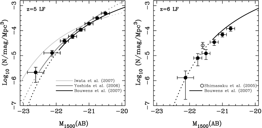
Figure 2: A comparison of our estimates of the bright end of the luminosity function at $z=5$ and $z=6$ with the Schechter function fits derived by recent literature studies. The left-hand panel compares our luminosity function estimate at $z=5$ with the results of Iwata et al. (2007), Yoshida et al. (2006) and Bouwens et al. (2007). The right-hand panel compares our luminosity function estimate at $z=6$ with the results of Shimasaku et al. (2005) and Bouwens et al. (2007). In each panel the literature luminosity function fits are plotted as solid curves where they are well constrained by data, and as dotted curves where there is no data, or only data with very large uncertainties.

5 The luminosity function at high redshift

Following the procedures outlined in the previous two sections, the UV-selected luminosity functions were estimated in two redshift intervals centred on $z=5$ and $z=6$. For the $z=5$ luminosity function we considered the redshift range $4.7\leq z\leq 5.3$ and for the $z=6$ luminosity function we considered the redshift range $5.7\leq z\leq 6.3$. These redshift ranges were chosen to be wide enough to include sufficient numbers of objects to provide a robust measurement of the bright end of the luminosity function, and narrow enough to limit the evolution of the luminosity function across each bin. The resulting estimates of the luminosity functions at $z=5$ and $z=6$ are shown in Fig. 1.

The advantages provided by the large area and deep optical+nearIR data available in the UDS/SXDS are immediately obvious from Fig. 1. As a result of the current data-set covering an area of 0.63 square degrees, it has been possible to robustly estimate the bright end of the luminosity function to absolute magnitudes as bright as $M_{1500}\simeq-22.5$ and $M_{1500}\simeq-22$ at $z=5$ and $z=6$ respectively. A second obvious feature of Fig. 1 is the significant evolution in the bright end of the luminosity function within the $5<z<6$ redshift interval; as previously demonstrated by Bouwens et al. (2007). From the data presented in Fig. 1 it is tempting to assume that this evolution is due entirely to a change in $M_{1500}^{\star}$ between $z=5$ and $z=6$ (a shift of $\Delta M_{1500}^{\star}\simeq 0.5$ magnitudes results in excellent agreement between the two luminosity functions). In fact, based on our data-set alone, it is not possible to determine whether the apparent evolution is due entirely to a change in $M_{1500}^{\star}$, or whether significant evolution in the normalisation ($\phi^{\star}$) is also occurring. However, the differential change in galaxy number density as a function of absolute magnitude does provide some information on the form of the luminosity function evolution. For example, while the number density of $M_{1500}\simeq-21$ galaxies only decreases by a factor of $\simeq 3$ between $z=5$ and $z=6$, the number density of $M_{1500}\simeq-22$ galaxies decreases by a factor of $\simeq 10$. In terms of Schechter function parameters, it is not possible to reproduce this change in luminosity function shape through evolution of $\phi^{\star}$ alone, and immediately confirms that some evolution of $M_{1500}^{\star}$ must be taking place. An attempt to quantify the relative contribution of evolution in $M_{1500}^{\star}$ and $\phi^{\star}$ is pursued in Section 5.2.

5.1 Comparison with previous studies

Before proceeding to explore the evolution of the luminosity function from $z=5$ to $z=6$ further, it is worthwhile comparing our results with those of recent studies in the literature.

Figure 3: A comparison of our luminosity function estimates at $z=5$ and $z=6$ with the equivalent estimates derived from deep HST imaging by Bouwens et al. (2007). It can be seen that the agreement between the two independent luminosity function estimates at both $z=5$ and $z=6$ is excellent. This figure illustrates the advantages provided by the wide area coverage of the current UDS/SXDS study. Although the unparallelled sensitivity of HST imaging provides tight constraints on the normalisation and faint-end slope of the $z\geq 5$ luminosity function, the wide area of the current UDS/SXDS study provides improved constraints on the bright end of the the luminosity function, and extends the dynamic range of the data by a factor of $\simeq 3$ in luminosity.

5.1.1 The $z\simeq 5$ luminosity function

The $z\simeq 5$ luminosity function has been investigated by several recent studies using both ground-based and HST imaging (e.g. Ouchi et al. 2004; Yoshida et al. 2006; Iwata et al. 2007; Oesch et al. 2007; Bouwens et al. 2007). As an illustration of the range of results which have recently been reported we show in Fig. 2a a comparison of our $z=5$ luminosity function estimate with the ground-based results of Yoshida et al. (2006) and Iwata et al. (2007), and the HST-based results of Bouwens et al. (2007). The Yoshida et al. (2006) study is based on deep Subaru Suprime-cam optical imaging data covering an area of $\simeq 0.25$ square degrees in the Subaru Deep Field. Yoshida et al. selected a large LBG sample centred on $z=4.7$, based on cuts in the $V-i^{\prime}$ vs $i^{\prime}-z^{\prime}$ colour-colour diagram, the reliability of which were confirmed via limited follow-up spectroscopy. The Schechter function fit derived by Yoshida et al. from their $z=4.7$ LBG sample is shown as the dark grey curve in Fig. 2a. It can be seen that our luminosity function estimate is in excellent agreement with the Yoshida et al. determination at $M_{1500}\leq-21.5$. At $M_{1500}\geq-21.5$ our number densities are somewhat lower than determined by Yoshida et al., although only by $\simeq 20$%. This difference is not very significant, and can largely be explained by the fact that the Schechter function fit derived by Yoshida et al. does not have a well constrained faint-end slope due to the lack of data fainter than $\simeq M_{1500}^{\star}$. We note here that the Yoshida et al. results at $z\simeq 5$ are very similar to those of Ouchi et al. (2004a), who analysed an combined SDF+SXDS data-set covering a larger area (0.35 square degrees) but with a magnitude limit $\simeq 0.5$ magnitudes brighter.

The solid black curve plotted in Fig. 2a is the Schechter function fit derived by Bouwens et al. (2007) from a sample of 1416 $V-$drop galaxies selected from a compilation of several deep HST imaging surveys (GOODS N+S, HUDF & HUDF-P). At $M_{1500}\geq-22$ our data are in excellent agreement with the Bouwens et al. luminosity function, which is remarkable given the very different techniques, data-sets and sky areas utilised by the two studies (the largest area in the Bouwens et al. study is the combined GOODS N+S fields; $\mbox{{\raisebox{-1.72218pt}{$\stackrel{{\scriptstyle<}}{{{\scriptstyle\sim}}}$}}}0.1$ square degrees). At the brightest magnitudes Fig. 2a suggests that our sample contains a higher number density of galaxies than predicted by the Bouwens et al. luminosity function. However, this is not unreasonable given that the large survey area of this study provides improved statistics on the bright end of the luminosity function, where the Bouwens et al. fit to the luminosity function is less well constrained.

Finally, in Fig. 2a we plot the recent luminosity function fit of Iwata et al. (2007) which is based on deep Subaru Suprime-cam imaging covering an area of $\simeq 0.35$ square-degrees (HDF-N and the J0053+1234 region). Based on cuts in the $V-I_{C}$ vs $I_{C}-z^{\prime}$ colour-colour diagram, Iwata et al. (2007) select 853 $z\simeq 5$ LBG candidates and derive the luminosity function fit shown as the light grey curve in Fig. 2a. It can be seen that our luminosity function estimate is in poor agreement with the Iwata et al. (2007) results, with the latter study finding a number density of objects at the brightest absolute magnitudes a factor of $\simeq 3$ higher than found here. It is difficult to understand how the large numbers of bright LBGs detected in the Iwata et al. study could be missing from our sample. Objects this bright would have very high signal-to-noise photometry in our data-set, and should return the most robust photometric redshifts. The Iwata et al. (2007) results are in good agreement with their previous estimate of the $z\simeq 5$ luminosity function (Iwata et al. 2003) and it has been suggested by several authors (e.g. Ouchi et al. 2004a; Yoshida et al. 2006; Bouwens et al. 2007) that the selection criteria used in Iwata et al. (2003, 2007) may allow contamination from low-redshift interlopers. We note that to produce number densities at $M_{1500}\leq-22$ as high as reported by Iwata et al. (2007), we would have to reinstate into our sample objects which have been excluded as suspected ultra-cool galactic stars due to their photometry being a poor match to any galaxy SED template

Figure 4: The best-fitting Schechter functions to the combined (ground-based+HST) data-sets at $z=5$ and $z=6$ are shown as the solid curves in the left-hand and right-hand panels respectively. During the fitting process the bright end of the luminosity function is constrained using the data from the current study (filled circles), while the faint end is constrained using the results of Bouwens et al. (2007), which are based on small area, but ultra-deep HST imaging. The best-fitting Schechter function parameters are listed in Table 1.

5.1.2 The $z\simeq 6$ luminosity function

Previous constraints on the $z\simeq 6$ luminosity function have been based, virtually exclusively, on the deep HST imaging available in the two GOODS regions, the Hubble Ultra-Deep Field (HUDF) and the HUDF parallel fields (e.g. Bunker et al. 2004; Dickinson et al. 2004; Yan & Windhorst 2004; Malhotra et al. 2005; Bouwens et al. 2006, 2007). In Fig. 2b we show the Schechter function fit to the $z\simeq 6$ luminosity function derived by Bouwens et al. (2007) from a sample of 627 $i-$dropouts selected from a compilation of the deepest available HST imaging data. Fig. 2b shows that our estimate of the $z=6$ luminosity function is in reasonable agreement with the luminosity function fit of Bouwens et al. (2007), although our number densities are lower by $\simeq 40$% in the region around $M_{1500}\simeq-21$, where the Bouwens et al. luminosity function fit is still well constrained by data. However, this discrepancy is only apparent in comparison to the Schechter function fit derived by Bouwens et al., and the actual data from the two studies are in excellent agreement (see Fig. 3b). In Fig. 2b we also show the number density of objects at $M_{1500}=-21.6$ derived by Shimasaku et al. (2005), based on a sample of 12 objects selected using imaging of the Subaru Deep Field with two medium-band $z-$filters. The Shimasaku et al. estimate is a factor of $\simeq 2$ higher than our estimated number density at $M_{1500}=-21.6$. The source of this discrepancy is not clear. Given the rigorous nature of their selection criteria, it seems unlikely that the Shimasaku et al. sample is contaminated by interlopers at the $\simeq 50$% level. However, the survey area covered by this work is a factor of $\simeq 3$ larger than that of the Shimasaku study, so it is likely that the apparent off-set is simply due to a combination of statistical errors and cosmic variance.

5.2 Combining the ground-based and HST data-sets

Although the results of the present study provide much improved constraints on the bright end of the luminosity function at $z=6$ and $z=5$, they do not reach faint enough to constrain the normalisation or faint-end slope of the $z\geq 5$ luminosity function. Consequently, in this section we explore the possibility of providing an improved measurement of the evolution of the luminosity function between $z=5$ and $z=6$ by combining our results with those of the HST-based study of Bouwens et al. (2007). In Fig. 3 we show a comparison of our luminosity function estimates at $z=5$ and $z=6$ with those of Bouwens et al. (2007). It can be seen that in the absolute magnitude range common to both studies the two, independent, estimates of the luminosity functions are in excellent agreement. Motivated by this agreement, it was decided to combine our results with those of Bouwens et al. (2007) to derive Schechter function fits to the luminosity function at $z=5$ and $z=6$ based on data spanning a factor of $\simeq 100$ in luminosity.

5.2.1 Fitting the luminosity functions

The adopted procedure was to use a maximum likelihood technique to fit a Schechter function to a finely sampled grid on the apparent $z^{\prime}-$band magnitude $-$ redshift plane $(m_{z}-z)$. To fit the luminosity function at $z=5$ the grid was populated within the redshift interval $4.7<z<5.3$ and the apparent $z^{\prime}-$band magnitude range $23<m_{z}<29$. In the magnitude range $23<m_{z}<26$ the grid was populated using the data from this study, while in the magnitude range $26<m_{z}<29$ the grid was populated according to the Schechter function fit to the $z=5$ luminosity function derived by Bouwens et al. (2007). This process was repeated to fit the $z=6$ luminosity function, with the exception that the redshift range considered was $5.7<z<6.3$. The fitting procedure was to maximise the following likelihood function:

$$\log L=\Sigma_{i,j}n_{i,j}\log p_{i,j}$$ (4)

where $n_{i,j}$ is the number of galaxies in cell $(i,j)$ and $p(i,j)$ is the probability of finding a galaxy within cell $(i,j)$ given the choice of model parameters. In this context, the probability $p(i,j)$ is naturally defined as $n_{p}(i,j)/\Phi_{z}$, where $n_{p}(i,j)$ is the predicted number of galaxies within cell $(i,j)$, for a given set of model parameters, and $\Phi_{z}$ is the corresponding integrated luminosity function.

5.2.2 Results

The best-fitting Schechter functions to the combined ground-based+HST data-sets at $z=5$ and $z=6$ are shown as the solid curves in Fig. 4. The best-fitting Schechter function parameters and their associated uncertainties are reported in Table 1, and the $1\sigma,2\sigma$ and $3\sigma$ confidence regions around the best-fitting values of the faint-end slope and characteristic magnitude are plotted in Fig. 5.

It can be seen from Fig. 4 that a Schechter function provides a good description of luminosity function at $z=5$ and $z=6$ over the full luminosity range ($\geq 5$ magnitudes) sampled by the combined ground-based+HST data-set. A comparison of the best-fitting Schechter function parameters derived here (Table 1) with those reported by Bouwens et al. (2007) shows that, at both redshifts, our best-fitting parameters are within the $1\sigma$ uncertainties reported by the earlier study. With respect to the faint-end slope and normalisation this is unsurprising, given that the constraints on these two parameters are largely provided by the deeper HST imaging data. However, the principle advantage provided by fitting the combined data-set is the improved constraints on the value of $M^{\star}_{1500}$; particularly at $z=6$. Our results suggest that $M^{\star}_{1500}$ dims by $0.69\pm 0.16$ magnitudes between $z=5$ and $z=6$. This is more dramatic than, although still completely consistent with, the dimming of $0.40\pm 0.23$ suggested by the Schechter function fits derived by Bouwens et al. (2007). With respect to the normalisation of the luminosity function, our results suggest that $\phi^{\star}$ increases by a factor of $\simeq 2$ between $z=5$ and $z=6$, although the comparatively large uncertainty on the normalisation of the Schechter function at $z=6$ means that this evolution is not statistically significant ($<2\sigma)$. As expected, our fit to the combined ground-based+HST data-set confirms the Bouwens et al. (2007) result that the faint-end slope of the luminosity function at $z\geq 5$ is steep ($\alpha\simeq-1.7$) and shows no sign of evolution in the redshift interval $5<z<6$.

Figure 5: Constraints on the faint-end slope and characteristic magnitude of the luminosity function at $z=5$ and $z=6$ derived via maximum likelihood fitting of the combined (ground-based+HST) data-set. The location of the best-fitting parameters at each redshift are shown by filled circles, and the plotted contours indicate the $1\sigma,2\sigma$ and $3\sigma$ confidence regions.

Table 1: The best-fitting Schechter function parameters from our maximum likelihood fitting of the combined (ground-based+HST) luminosity function data-sets at $z=5$ and $z=6$. The errors on the faint-end slope and characteristic magnitude have been derived from the likelihood ratio contours shown in Fig. 5. The values of $\phi^{\star}$ and their associated errors have been calculated by fitting the number counts in each redshift interval.

Redshift	$\phi^{\star}$/Mpc-3	M${}^{\star}_{1500}$	$\alpha$
5.0	$(9.4\pm{1.9})\times 10^{-4}$	$-20.73\pm{0.11}$	$-1.66\pm{0.06}$
6.0	$(1.8\pm{0.5})\times 10^{-3}$	$-20.04\pm{0.12}$	$-1.71\pm{0.11}$

6 Clustering analysis

In this section we evaluate the 2-point angular correlation function for those LBGs in our sample with primary photometric redshift solutions in the interval $5.0<z<6.0$. To measure the angular correlation function $\omega(\theta)$ and estimate the related poissonian errors we used the Landy & Szalay (1993) estimators. The correlation function derived from our $5.0<z<6.0$ LBG sample is shown in Fig. 6. The best fit for the angular correlation is assumed to be a power-law as in Groth & Peebles (1977):

$$\omega(\theta)=A_{\omega}(\theta^{-\delta}-C_{\delta})$$ (5)

with the amplitude at 1 degree $A_{\omega}=13.0^{+5.9}_{-4.1}\times 10^{-3}$, the slope $\delta=0.72\pm 0.08$, and the integral constraint due to the limited area of the survey $C_{\delta}=2.34$ (determined over the unmasked area). It should be noted that because the contamination of our $5<z<6$ LBG sample from low-redshift interlopers is securely $<10\%$ we have made no correction for dilution of the clustering signal.

Figure 6: 2-point angular correlation function determined for our sample of $5.0<z<6.0$ LBGs, with its fitted power-law (solid line). The best-fitting parameters for the amplitude and slope are indicated. The dashed line represents the power-law fitting only the largest scales measurements ($\theta>10^{\prime\prime}$) assuming a slope fixed to $\delta=0.6$. The plot inset presents the $\chi^{2}$ minimisation to estimate the best-fitting values of $A_{\omega}$ and $\delta$, with contours showing the $1\sigma$ and $3\sigma$ confidence levels.

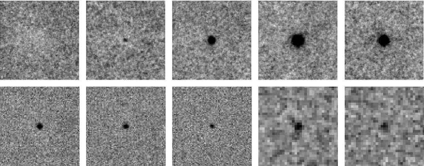
Figure 7: Postage stamps of the stacked imaging data for the 754 LBGs with primary photometric redshift solutions in the range $5.0<z<6.0$. From top left to bottom right the first eight postage stamps show the stacked $BVRi^{\prime}z^{\prime}JHK$ data. The final two postage stamps show the stacked IRAC data at 3.6$\mu$m and 4.5$\mu$m. It can be seen from the second panel that the stacking analysis produces a very faint detection in the $V-$band ($V=32.3\pm 0.6$). This is not unexpected given that the Lyman-limit does not pass fully through the Subaru $V-$band filter until $z=5.5$. All the postage stamps have dimensions of 20^′′$\times$ 20^′′, and are shown on a linear grey-scale in the range $\pm 5\sigma$ (where $\sigma$ is the rms sky noise). The $H-$band photometry recently became available in UKIDSS DR3, and was only used in the stacking analysis.

In Fig. 6 we also indicate the best-fitting curve determined using only the largest scale measurements ($\theta>10^{\prime\prime}$) and a fixed value for the slope of $\delta=0.6$. Based on a sample of $z\simeq 5$ LBGs selected from the GOODS fields, Lee et al. (2006) find that their angular clustering measurments show a strong transition on the smallest scales ($\theta<10^{\prime\prime}$), indicative of a intra/inter dark matter halo transition, while on larger scales the angular correlation is well approximated by a power-law with a slope of $\delta=0.6$. However, as can be seen from Fig. 6, our results are consistent with a value of $\delta=0.6$ on large scales, and only present a non-significant deviation from this slope on the smallest scales ($\theta=3.6^{\prime\prime}$ corresponding to $\sim 20h^{-1}_{70}$kpc).

In order to compare the clustering of galaxy populations at different redshifts it is necessary to derive spatial correlation measurements. Using the redshift distribution of our sample we can derive the correlation length using the relativistic Limber equation (Magliocchetti & Maddox 1999) and, in addition, derive a linear bias estimation (Magliocchetti et al. 2000) assuming that the dark matter behaves as predicted by linear theory. To perform this calculation we have adopted the redshift distribution for our sample as derived from integrating over the redshift probability density functions for those objects with primary photometric redshift solutions in the interval $5.0<z<6.0$. The correlation length can then be evaluated by fixing the slope of the correlation function to $\gamma=1+\delta=1.72$. This calculation produces a measurement of $r_{0}=8.1^{+2.1}_{-1.5}\,h^{-1}_{70}$Mpc for the correlation length and a value of $b=5.4^{+1.2}_{-0.8}$ for the linear bias. Although we consider this to be our best estimate of the clustering properties of the sample, we note that if we instead adopt the redshift distribution based on the best-fitting photometric redshifts alone ($\bar{z}=5.38$; see Fig A2) we derive slightly higher, although consistent, values of $r_{0}=9.6^{+2.5}_{-1.8}\,h^{-1}_{70}$Mpc and $b=6.2^{+1.4}_{-1.0}$ for the correlation length and linear bias respectively.

It is of interest to compare our clustering results for $z^{\prime}<26.0$ LBGs in the redshift interval $5.0<z<6.0$ with recent literature results for LBG samples with similar limiting magnitudes and mean redshifts. Our results are in good agreement with Ouchi et al. (2004b) who derived a correlation length of $r_{0}=8.4^{+1.8}_{-2.4}\,h^{-1}_{70}$Mpc for a sample of $z^{\prime}<25.8$ LBGs with a mean redshift of $\bar{z}=4.7$ in the Subaru Deep Field. In addition, our results are in agreement with those of Overzier et al. (2006) who derived a correlation length of $r_{0}=9.6^{+4.0}_{-5.6}\,h^{-1}_{72}$Mpc for a sample of $z_{850}<27.0$ LBGs with a mean redshift of $\bar{z}=5.9$ in the GOODS fields. Finally, our results are also in good agreement with those of Lee et al. (2006), who derived a value of $r_{0}=7.5^{+1.1}_{-1.0}\,h^{-1}_{70}$Mpc (fixed slope of $\delta=0.6$) from their sample of $z_{850}<26.0$ LBGs in the GOODS fields with a mean redshift of $\bar{z}=4.9$.

Based on the predictions of dark matter halo models (Sheth et al. 2001; Mo & White 2002), and assuming a one-to-one correspondance between galaxies and halos, we infer that our $5.0<z<6.0$ LBGs are likely to be hosted by dark matter halos with masses of $M_{DM}\geq 10^{11.5-12}M_{\odot}$, comparable to what is observed for $L>L^{\star}$ LBGs at $z\sim 3-4$.

7 Stacking analysis

In this section we explore the possibility of estimating the typical stellar mass of our $5<z<6$ LBGs from a stacking analysis of the available optical+nearIR imaging data. The aim is to test whether the typical stellar mass is compatible with the dark matter halo mass suggested by the clustering analysis.

In Fig. 7 we show 20^′′$\times$ 20^′′  postage stamps produced by taking a median stack of the available imaging data, centred on the positions of the 754 LBG candidates with primary photometric redshift solutions in the interval $5.0<z<6.0$. There are several features of Fig. 7 which are worthy of comment. Firstly, in the stack of the $B-$band photometry the LBG candidates are robustly non-detected ($B\leq 33$; $1\sigma$), as expected from our initial selection criteria. Secondly, it can be seen that there is a faint detection in the stacked $V-$band data. However, the $V-$band detection is very faint ($V=32.3\pm 0.6$) and is expected given that the Lyman-limit does not pass out of the Subaru Suprime-Cam $V-$filter until $z=5.5$. Finally, the two panels on the lower right of Fig. 7 show the results of stacking the available Spitzer IRAC data at $3.6\mu$m and $4.5\mu$m from the SWIRE survey (Lonsdale et al. 2003). Although relatively shallow, the SWIRE data is deep enough to produce detections at $3.6\mu$m and $4.5\mu$m in the median stack. Together with the robust photometry from the stacked $JHK$ imaging data, it is the extra wavelength coverage provided by the detections at $3.6\mu$m and $4.5\mu$m which will allow us to place useful constraints on the typical stellar mass of the $5<z<6$ LBGs.

7.1 SED fitting

Using the same procedure as described in Section 3.1, the best-fitting galaxy template to the stacked photometry is shown in Fig. 8. It can be seen from the lower panel of Fig. 8 that the fit to the stacked photometry provides a robust redshift solution at $z=5.43^{+0.05}_{-0.10}$ and that any alternative low-redshift solution is securely ruled out. The best-fitting SED template has an age of 400 Myrs, consistent with a typical formation redshift of $z\simeq 7-8$, and no intrinsic reddening ($A_{V}=0$). By considering the range of SED templates which provide an acceptable fit to the stacked photometry, we calculate that the stellar mass of the LBG stack is $\log_{10}({\rm{M}/\mbox{\,$\rm M_{\odot}$}})=10.0^{+0.2}_{-0.4}$ (Salpeter IMF).

7.2 Dark matter to stellar mass ratio

Although the uncertainties in the determination of the typical stellar and dark halo mass for the $5<z<6$ LBG sample are obviously large, combined with the results of the clustering analysis reported in the previous section, the SED fit to the stacked photometry suggests that the typical dark matter to stellar mass ratio for the $5<z<6$ LBGs is $\frac{M_{DM}}{M_{stars}}\simeq 30-100$. Given that our LBG sample are exclusively drawn from the bright end of the $5<z<6$ luminosity function it would seem reasonable to assume that they will evolve into objects occupying the high-mass end of the low-redshift galaxy stellar mass function (i.e. $M\geq M^{\star}_{stars}$). In which case, it is noteworthy that $\frac{M_{DM}}{M_{stars}}\simeq 50$ is in good agreement with the measured value for Luminous Red Galaxies (LRGs) in the SDSS from galaxy-galaxy lensing (Mandelbaum et al. 2006). Moreover, $\frac{M_{DM}}{M_{stars}}\simeq 50$ is also in good agreement with the predicted mean value for low-redshift LRGs from recent semi-analytic galaxy formation models (e.g. Almeida et al. 2008)

Figure 8: The upper panel shows the SED fit to the stacked imaging data of those LBG candidates with primary photometric redshift solutions in the range $5.0<z<6.0$. In addition to the $BVRi^{\prime}z^{\prime}JK$ photometry used in the selection of the LBG sample, the stacked data includes $H-$band (which recently became available in UKIDSS DR3), and detections at 3.6$\mu$m and 4.5$\mu$m from stacking the Spitzer SWIRE data covering the UDS. The bottom panel shows $\chi^{2}$ versus redshift for the SED fit to the stacked data. As expected, the SED fit has a very robust solution at $z=5.43^{+0.05}_{-0.10}$ and no plausible low-redshift solutions are evident.

8 The stellar mass function

Although it remains a possibility that a substantial population of massive, comparatively red, objects exist at high redshift, it seems likely that the luminous ($L\geq L^{\star}$) LBGs selected in this study are amongst the most massive galaxies in existence at $5<z<6$. As such, their number densities and stellar masses have the potential to provide constraints on the latest generation of galaxy evolution models.

In Fig. 9 we show an estimate of the galaxy stellar mass function at $5<z<6$ based on combining the luminosity function fits presented in Section 5 with the results of the stacking analysis presented in Section 7. The adopted procedure for estimating the stellar mass function is extremely straightforward. Based on the Schechter function fits to the luminosity function at $z=5$ and $z=6$, we have estimated the corresponding stellar mass function by simply multiplying the luminosity function fits by the mass-to-light ratio derived from our SED fit to the stacked LBG imaging data. In Fig. 9 the upper envelope of the grey shaded area is our estimate of the stellar mass function at $z=5$, while the lower envelope is our corresponding estimate at $z=6$ (both include the $1\sigma$ uncertainties on the best-fitting Schechter luminosity function parameters). For comparison we also plot the stellar mass function estimates at $z=5.3$ based on the De Lucia & Blaizot (2007) and Bower et al. (2006) semi-analytic galaxy formation models (thick and thin curves respectively). In order to perform a fair comparison, we have shifted our stellar mass function estimates to lower masses by a factor of 1.8, to account for the fact that the De Lucia & Blaizot (2007) and Bower et al. (2006) models are based on IMFs which typically return stellar masses a factor of $\simeq 1.8$ lower than our Salpeter-based estimates (De Lucia & Blaizot 2007). Finally, for reference, the dashed curve in Fig. 9 is the stellar mass function at $z\simeq 0$ from Cole et al. (2001).

The mass function predictions from the Bower et al. (2006) and De Lucia & Blaizot (2007) models are in good agreement, at least qualitatively, with our observational estimate. The general agreement between our estimate, based on the UV-selected luminosity function, and the model predictions suggests that LBGs constitute the majority of the stellar mass density at $z\geq 5$ and, if the model predictions are correct, a putative population of reddened/older galaxies at $5<z<6$ does not dominate the stellar mass density. Compared to the $z\simeq 0$ mass function, our estimate of the high-redshift stellar mass function suggests that the number density of $\simeq 10^{10}\mbox{\,$\rm M_{\odot}$}$ and $\simeq 10^{11}\mbox{\,$\rm M_{\odot}$}$ galaxies in place by $z\simeq 5$ is $\simeq 10$% and $\simeq 0.1$% of its local value respectively.

8.1 Stellar mass density

Given that we have estimated the stellar mass function at $z=5$ and $z=6$ by simply applying a constant mass-to-light ratio derived from our stacking analysis, it is obviously somewhat speculative to proceed to estimate the co-moving stellar mass density.

However, for completeness, integrating our stellar mass function estimates down to a mass limit of $M\geq 10^{9.5}\mbox{\,$\rm M_{\odot}$}$ provides stellar mass density estimates of $\simeq 1\times 10^{7}\mbox{\,$\rm M_{\odot}$}$ Mpc^-3 and $\simeq 4\times 10^{6}\mbox{\,$\rm M_{\odot}$}$ Mpc^-3 at $z=5$ and $z=6$ respectively (Salpeter IMF). It was decided to integrate our stellar mass function down to a limit of $M\geq 10^{9.5}\mbox{\,$\rm M_{\odot}$}$ for two reasons. Firstly, a mass limit of $M\geq 10^{9.5}\mbox{\,$\rm M_{\odot}$}$ corresponds well to the mass limits of Stark et al. (2007) and Yan et al. (2006), who previously estimated the stellar mass density at $z=5$ and $z=6$ respectively. Secondly, given that our data-set provides no information on the mass-to-light ratios of objects with masses smaller than $10^{9.5}\mbox{\,$\rm M_{\odot}$}$, it would clearly be ill advised to extrapolate to smaller stellar masses.

Our stellar mass density estimate at $z=5$ is in reasonable agreement with the estimate of $6\times 10^{6}\mbox{\,$\rm M_{\odot}$}$ Mpc^-3 derived by Stark et al. (2007) from a combined sample of spectroscopic and photometrically selected galaxies in the southern GOODS field. Moreover, our estimate of the stellar mass density at $z=6$ is in agreement with the lower limit of $1.1-6.7\times 10^{6}\mbox{\,$\rm M_{\odot}$}$ Mpc^-3 derived by Yan et al. (2006), based on a sample of $i-$drop galaxies in the north and south GOODS fields. The stellar mass densities quoted by both Stark et al. (2007) and Yan et al. (2006) are also based on a Salpeter IMF.

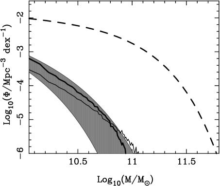
Figure 9: Estimates of the stellar mass function in the redshift interval $5<z<6$. The upper envelope of the grey shaded area is our estimate of the stellar mass function at $z=5$, and the lower envelope is our corresponding estimate at $z=6$ (both include the $1\sigma$ uncertainties on the best-fitting Schechter luminosity function parameters). The thick and thin solid lines show the estimated stellar mass function at $z=5.3$ derived from a combination of the Millennium N-body simulation and the semi-analytic galaxy formation models of De Lucia et al. & Blaizot (2007) and Bower et al. (2006) respectively. The upper dashed curve is the stellar mass function measurement at $z\simeq 0$ from Cole et al. (2001).

9 Conclusions

In this paper we have reported the results of a study of a large sample of luminous ($L\geq L^{\star}$) LBGs in the redshift interval $4.7<z<6.3$. By employing a photometric redshift analysis of the available optical+nearIR data we have derived improved estimates of the bright end of the UV-selected luminosity function at $z=5$ and $z=6$. Moreover, by combining our new results with those based on deeper, but small area, HST data we have derived improved constraints on the best-fitting Schechter function parameters at $z=5$ and $z=6$. In addition, by studying the angular clustering properties of our sample we have determined that luminous LBGs at $5<z<6$ typically lie in dark matter halos with masses of $10^{11.5-12}\mbox{\,$\rm M_{\odot}$}$. Finally, based on the results of a stacking analysis, we have estimated the galaxy stellar mass functions and integrated stellar mass densities at $z=5$ and $z=6$. Our main conclusions can be summarised as follows:

1. Our new determination of the bright end of the high-redshift luminosity function confirms that significant evolution occurs over the redshift interval $5<z<6$. Based on our results it is clear that the luminosity function evolution cannot be described by evolution in normalisation ($\phi^{\star}$) alone, and that some level of evolution in $M^{\star}_{1500}$ is also required.

2. A comparison of our new results with those in the literature demonstrates that, within the magnitude range where the two studies overlap, our estimates of the luminosity function at $z=5$ and $z=6$ are in excellent agreement with those derived from ultra-deep HST imaging data by Bouwens et al. (2007).

3. By combining our estimate of the bright end of the luminosity function with the corresponding estimates of the faint end by Bouwens et al. (2007), it is possible to fit the luminosity function at $z=5$ and $z=6$ over a luminosity range spanning a factor of $\simeq 100$. Based on this combined ground-based+HST data-set we find the following best-fitting Schechter function parameters: $M_{1500}^{\star}=-20.73\pm 0.11,\phi^{\star}=0.0009\pm 0.0002\,{\rm Mpc}^{-3}$ and $\alpha=-1.66\pm 0.06$ for the luminosity function at $z=5$, and $M_{1500}^{\star}=-20.04\pm 0.12,\phi^{\star}=0.0018\pm 0.0005\,{\rm Mpc}^{-3}$ and $\alpha=-1.71\pm 0.11$ at $z=6$.

4. These results are consistent with the corresponding Schechter function parameters derived by Bouwens et al. (2007) although, due to the improved statistics at the bright end provided by our wide survey area, the fits to the combined ground-based+HST data-set provide improved constraints on the evolution of $M^{\star}_{1500}$ in particular.

5. An analysis of their angular clustering properties demonstrates that luminous $L\geq L^{\star}$ LBGs at $5<z<6$ are strongly clustered, with a correlation length of $r_{0}=8.1^{+2.1}_{-1.5}\,h^{-1}_{70}$Mpc. Comparison of these clustering results with theoretical models suggests that these LBGs typically reside in dark matter halos with masses of $\simeq 10^{11.5-12}\mbox{\,$\rm M_{\odot}$}$.

6. An SED fit to a stack of the available optical+NearIR data for our sample suggests that luminous LBGs at $5<z<6$ have typical stellar masses of $\simeq 10^{10}\mbox{\,$\rm M_{\odot}$}$. Combined with the results of the clustering analysis this suggests that the typical ratio of dark matter to stellar mass for luminous LBGs at $5<z<6$ is $\frac{M_{DM}}{M_{stars}}\simeq 30-100$.

7. Assuming that the mass-to-light ratio derived from the SED fit to the stacked LBG imaging data is representative, we use our best-fitting Schechter function parameters for the $z=5$ and $z=6$ luminosity functions to estimate the corresponding stellar mass functions. Although clearly subject to large uncertainties, our stellar mass function estimates are consistent with the latest predictions of the semi-analytic galaxy formation models of De Lucia & Blaizot (2007) and Bower et al. (2006).

8. Based on our stellar mass function estimates we calculate that the stellar mass in place at $z=5$ and $z=6$ is $\simeq 1\times 10^{7}\mbox{\,$\rm M_{\odot}$}$ Mpc^-3 and $\simeq 4\times 10^{6}\mbox{\,$\rm M_{\odot}$}$ Mpc^-3 respectively. Although uncertain, these independent estimates of the integrated stellar mass density are consistent with the results of studies utilising the ultra-deep Spitzer IRAC data in the GOODS fields (Stark et al. 2007; Yan et al. 2006).

10 acknowledgments

The authors would like to thank the anonymous referee whose comments and suggestions significantly improved the final version of this manuscript. RJM and OA would like to acknowledge the funding of the Royal Society. MC and SF would like to acknowledge funding from STFC. We are grateful to the staff at UKIRT and Subaru for making these observations possible. We also acknowledge the Cambridge Astronomical Survey Unit and the Wide Field Astronomy Unit in Edinburgh for processing the UKIDSS data.

Appendix A Luminosity function estimates: technical details

When deriving our estimates of the LBG luminosity functions at $z=5$ and $z=6$ in Section 4 we employed several techniques which differ somewhat from those which have been commonly adopted in previous literature studies. Consequently, it is perhaps instructive to investigate what influence these techniques have on the derived luminosity function estimates. In this section we first investigate the influence of our completeness corrections, before proceeding to investigate the influence of our decision to make use of the full photometric redshift probability density function for each LBG candidate.

A.1 Correction factor

As previously discussed in Section 4, to estimate the LBG luminosity function at $z=5$ and $z=6$ we used the $V/V_{max}$ maximum likelihood estimator of Schmidt (1968), adapted to incorporate the photometric redshift probability density function of each LBG candidate. Consequently, within a given redshift interval ($z_{min}<z<z_{max}$), our estimate of the luminosity function within a given absolute magnitude bin was:

$$\phi(M)=\sum_{i=1}^{i=N}\int^{z_{2}(m_{i})}_{z_{1}(m_{i})}\frac{C_{i}(m_{i},z^{\prime})P_{i}(z^{\prime})\delta z^{\prime}}{V_{i}^{max}(m_{i},z^{\prime})}$$ (6)

where the summation runs over the full sample, and $z_{1}\rightarrow z_{2}$ is the redshift range within which a candidate’s absolute magnitude lies within the magnitude bin in question. As described in detail in Section 4, the quantity $C_{i}(m_{i},z)$ is a correction factor derived from realistic monte-carlo simultions of the evolving LBG population, and accounts for sample incompleteness, object blending and contamination from objects photometrically scattered into the sample from faint-ward of the $z^{\prime}-$band magnitude limit.

To illustrate the influence of the correction factor we show in Fig A1 our estimates of the $z=5$ and $z=6$ LBG luminosity functions with and without the inclusion of $C_{i}(m_{i},z)$. In Fig A1 the open and filled black symbols are the estimates of the $z=5$ and $z=6$ luminosity functions including the correction factor (identical to the estimates displayed in Fig 1), while the grey symbols are the equivalent estimates setting $C_{i}(m,z)=1$. It can be seen from Fig A1 that the correction factor does not have a significant impact on the shape of the luminosity function estimates. At the bright end, where our sample is most complete, the off-set between the black and grey data-points is simply due to the $\simeq 15$% correction for objects lost due to blending in the crowded Subaru images. In the faintest absolute magnitude bins the inclusion of the correction factor boosts the number densities by a roughly constant factor of $\simeq 30$% (0.1 dex). This effect is due to a balance between the increasing positive correction that has to be made for incompleteness as the data approach the $z^{\prime}=26$ magnitude limit, and the increasingly negative correction that has to be made for objects photometrically scattered into the sample from faint-ward of the magnitude limit.

A.2 Comparing different photometric redshift techniques

When deriving our estimates of the LBG luminosity functions at $z=5$ and $z=6$ in Section 4 we used the full photometric redshift probability density functions provided by our SED template fitting code in order to make full use of the available information. In this section we investigate the influence of this technique on the derived luminosity function estimates. Of particular interest is to investigate how the derived luminosity function estimates change if we simply treat the best-fitting photometric redshift for each LBG as unique, and ignore the possibility of secondary redshift solutions.

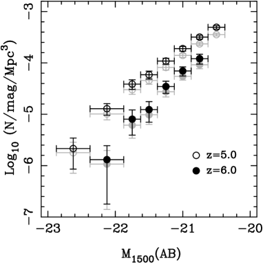
Figure 10: Estimates of the bright end of the UV-selected luminosity function at $z=5$ and $z=6$. The open and filled black data-points are derived using Eqn A1, including the correction factor $C_{i}(m_{i},z)$, and are identical to those presented in Fig 1. The grey data-points are the corresponding estimates derived by setting $C_{i}(m_{i},z)$=1 (see text for discussion).

Figure 11: A comparison of the LBG redshift distributions as derived using the best-fitting photometric redshifts (left-hand column) and integrating over the full redshift probability density function (right-hand column). The appropriate redshift range and the number of objects lying within that range are listed in the top right-hand corner of each panel.

A.2.1 Redshift distributions

The first straightforward comparison of the two techniques is to compare the estimated redshift distributions. In Fig A2 we show the LBG redshift distributions in the three redshift intervals utilised in this paper: $4.7<z<5.3$, $5.0<z<6.0$ and $5.7<z<6.3$. The redshift distributions shown in the left-hand column are derived by treating the best-fitting photometric redshift for each LBG as unique and robust. The redshift distributions shown in the right-hand column are derived by integrating over the full redshift probability density functions as done in Section 4. The number of objects included in each redshift distribution is listed in the top right-hand corner of each panel.

Although the redshift distributions derived via both techniques are broadly similar, it can be seen from Fig A2 that they do differ in detail. Perhaps the most noticeable difference is that adopting the best-fitting photometric redshifts alone predicts $\simeq 50$% more objects in the highest redshift interval ($5.7<z<6.3$). Armed with this information we now proceed to investigate how the differences in redshift distributions affect the estimated luminosity functions.

A.2.2 Luminosity function estimates

In Fig A3 we show estimates for the bright end of the $z=5$ and $z=6$ LBG luminosity functions. The left-hand panels show the estimates derived in Section 4 by adopting the photometric redshift probability density function for each LBG. The right-hand panels show the luminosity function estimates derived from simply adopting the best-fitting photometric redshift for each source. In each panel we also plot the maximum likelihood Schechter function fits to the LBG luminosity function at either $z=5$ or $z=6$ as derived in Section 5.2.

It can be seen from Fig A3 that the estimate of the $z=5$ luminosity function is virtually identical using both techniques. This is as expected given the similarity of the $4.7<z<5.3$ redshift distributions shown in the top panel of Fig A2, and demonstrates that the photometric redshifts at $z\simeq 5$ are sufficiently robust that both techniques lead to indistinguishable conclusions. In contrast, although the two luminosity function estimates at $z=6$ are clearly consistent, there are differences in detail. Specifically, it can be seen from Fig A3 that the luminosity function estimate based on the best-fitting photometric redshifts predicts more objects in the three faintest absolute magnitude bins. This effect is entirely consistent with the differences between the $5.7<z<6.3$ redshift distributions shown in Fig A2, which demonstrate that using the best-fitting photometric redshifts alone predicts $\simeq 50$% more objects at $z\simeq 6$.

In conclusion, it is clear from the information displayed in Figs A2 & A3 that the only substantive difference between the two techniques is for the faintest LBGs at $z\simeq 6$. This is perhaps to be expected, given that these are the very objects for which the best-fitting photometric redshifts are least robust, and was the primary motivation for exploiting the extra information contained within the full redshift probability density function for each object. However, the good agreement between the luminosity function estimate shown in the bottom right panel of Fig A3 and the best-fitting Schechter function derived in Section 5.2 confirms that adopting either technique would lead to the same conclusions regarding the form, and evolution, of the LBG luminosity function between $z=5$ and $z=6$.

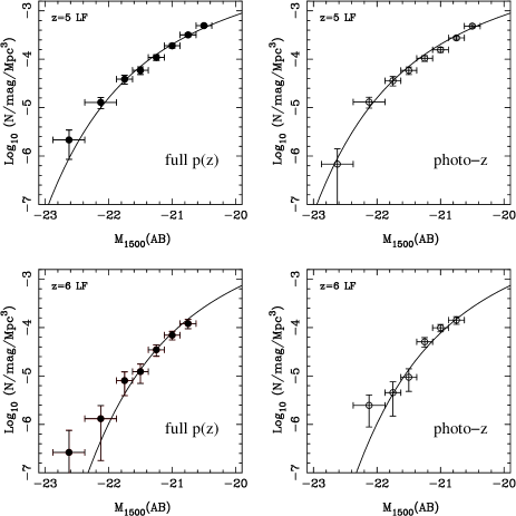
Figure 12: A comparison of the LBG luminosity function estimates at $z=5$ and $z=6$ resulting from using the full redshift probability density function for each object (left-hand plots) and the best-fitting photometric redshifts alone (right-hand plots). The top two plots show the different luminosity function estimates at $z=5$, while the bottom two plots show the different luminosity function estimates at $z=6$. The maximum likelihood fits to the $z=5$ and $z=6$ luminosity functions derived in Section 5.2 are plotted in the top and bottom panels respectively.

References

- [1] Almeida C., Baugh C.M., Wake D.A., Lacey C.G., Benson A.J., Bower R.G., Pimbblet K., 2008, MNRAS, in press, arXiv:0710.3557 [astro-ph]
- [2] Bertin E., Arnouts S., 1996, A&AS, 117, 393
- [3] Bolzonella M., Miralles J.M., Pelló, 2000, A&A, 363, 476
- [4] Bouwens R.J., Illingworth G.D., Blakeslee J.P., Franx M., 2006, ApJ, 653, 53
- [5] Bouwens R.J., Illingworth G.D., Franx M., Ford H., 2007, ApJ, 670, 928
- [6] Bouwens R.J., Illingworth G.D., Franx M., Ford H., 2008, ApJ, submitted, arXiv:0803.0548 [astro-ph]
- [7] Bower R.G., Benson A.J., Malbon R., Helly J.C., Frenk C.S., Baugh C.M., Cole S., Lacey C.G., 2006, MNRAS, 370, 645
- [8] Bruzual G., Charlot S., 2003, MNRAS, 344, 1000
- [9] Bunker A.J., Stanway E.R., Ellis R.S., McMahon R.G., 2004, MNRAS, 355, 374
- [10] Calzetti D., Armus L., Bohlin R. C., Kinney A. L., Koornneef J., Storchi-Bergmann T., 2000, ApJ, 533, 682
- [11] Casali M., et al., 2007, A&A, 467, 777
- [12] Cirasuolo M., et al., 2007, MNRAS, 380, 585
- [13] Cirasuolo M., McLure R.J., Dunlop J.S., Almaini O., Foucaud S., Simpson C., 2008, MNRAS, submitted, arXiv:0804.3471 [astro-ph]
- [14] Cole S., et al., 2001, MNRAS, 326, 255
- [15] De Lucia G., Blaizot J., 2007, MNRAS, 375, 2
- [16] Dickinson M., et al., 2004, ApJ, 600, L99
- [17] Dunlop J.S., Cirasuolo M., McLure R.J., 2007, MNRAS, 376, 1054
- [18] Eyles L.P., Bunker A.J., Stanway E.R., Lacy M., Ellis R.S., Doherty M., 2005, MNRAS, 364, 443
- [19] Furusawa H., et al., 2008, ApJS, 176, 1
- [20] Groth E.J., Peebles P.J.E., 1977, ApJ, 217, 385
- [21] Guhathakurta P., Tyson J.A., Majewski S.R., 1990, ApJ, 357, L9
- [22] Iye M., et al., 2006, Nature, 443, 186
- [23] Iwata I., Ohta K., Tamura N., Ando M., Wada S., Watanabe C., Akiyama M., Aoki K., 2003, PASJ, 55, 415
- [24] Iwata I., Ohta K., Tamura N., Akiyama M., Aoki K., Ando M., Kiuchi G., Sawicki M., 2007, MNRAS, 376, 1557
- [25] Hu E.M., McMahon R.G., Cowie L.L., 1999, ApJ, 521, L9
- [26] Landy S.D., Szalay A.S., 1993, ApJ, 412, 64
- [27] Lawrence A., et al., 2007, MNRAS, 379, 1599
- [28] Lee K.S., Giavalisco M., Gnedin O.Y., Somerville R.S., Ferguson H.C., Dickinson M., Ouchi M., 2006, ApJ, 642, 63
- [29] Lonsdale C.J., et al., 2003, PASP, 115, 897
- [30] Madau P., 1995, ApJ, 441, 18
- [31] Magliocchetti M., Maddoz S.J., 1999, MNRAS, 306, 988
- [32] Magliocchetti M., Bagla J.S., Maddox S.J., Lahav O., 2000, MNRAS, 314, 546
- [33] Malhotra S., et al., 2005, ApJ, 626, 666
- [34] Mandelbaum R., Seljak U., Kauffmann G., Hirata C.M., Brinkmann J., 2006, MNRAS, 368, 715
- [35] McLure R.J., et al., 2006, MNRAS, 372, 357
- [36] Mo H.J., White S.D.M., 2002, MNRAS, 336, 112
- [37] Moscardini L., Coles P., Lucchin F., Materrese S., 1998, MNRAS, 299, 95
- [38] Miyazaki S., et al., 2002, PASJ, 54, 833
- [39] Oesch P.A., et al., 2007, ApJ, 671, 1212
- [40] Oke J.B., Gunn J.E., 1983, ApJ, 266, 713
- [41] Ouchi M., et al., 2004a, ApJ, 611, 660
- [42] Ouchi M., et al., 2004b, ApJ, 611, 685
- [43] Ouchi M., et al., 2005, ApJ, 635, L117
- [44] Ouchi M., et al., 2008, ApJS, in press, arXiv:0707.3161 [astro-ph]
- [45] Overzier R.A., Bouwens R.J., Illingworth G.D., Franx M., 2006, ApJ, 648, L5
- [46] Reddy N.A., Steidel C.C., Pettini M., Adelberger K.L., Shapley A.E., Erb D.K., Dickinson M., 2008, ApJS, 175, 48
- [47] Rodighiero G., Cimatti A., Franceschini A., Brusa M., Fritz J., Bolzonella M., 2007, A&A, 470, 21
- [48] Sawicki M., Thompson D., 2006, ApJ, 642, 653
- [49] Schmidt M., 1968, ApJ, 151, 393
- [50] Shapley A.E., Steidel C.C., Pettini M., Adelberger K.L., 2003, ApJ, 588, 65
- [51] Shimasaku K., Ouchi M., Furusawa H., Yoshida M., Kashikawa N., Okamura S., 2005, PASJ, 57, 447
- [52] Sekiguchi K., et al., 2005, in Renzini A. & Bender R. ed., Multiwavelength mapping of galaxy formation and evolution. Springer-Verlag, Berlin, p82
- [53] Sheth R.K., Mo H.J., Tormen G., 2001, MNRAS, 323, 1
- [54] Stark D.P., Bunker A.J., Ellis R.S., Eyles L.P., Lacy M., 2007b, ApJ, 659, 84
- [55] Stark D.P., Ellis R.S., Richard J., Kneib J.P., Smith G.P., Santos M.R., 2007a, ApJ, 663, 10
- [56] Steidel C.C., Adelberger K.L., Giavalisco M., Dickinson M., Pettini M., 1999, ApJ, 519, 1
- [57] Taniguchi Y., et al., 2005, PASJ, 57, 165
- [58] Warren, S. J., et al., 2007, MNRAS, 375, 213
- [59] Yan H., Windhorst R.A., 2004, ApJ, 612, L93
- [60] Yan H., Dickinson M., Giavalisco M., Stern D., Eisenhardt P.R.M., Ferguson H.C., 2006, ApJ, 651, 24
- [61] Yoshida M., et al., 2006, ApJ, 653, 988