Greedy Forwarding in Dynamic Scale-Free Networks Embedded in Hyperbolic Metric Spaces

Abstract

We show that complex (scale-free) network topologies naturally emerge from hyperbolic metric spaces. Hyperbolic geometry facilitates maximally efficient greedy forwarding in these networks. Greedy forwarding is topology-oblivious. Nevertheless, greedy packets find their destinations with $100\%$ probability following almost optimal shortest paths. This remarkable efficiency sustains even in highly dynamic networks. Our findings suggest that forwarding information through complex networks, such as the Internet, is possible without the overhead of existing routing protocols, and may also find practical applications in overlay networks for tasks such as application-level routing, information sharing, and data distribution.

I Introduction

Routing information is the most basic and, perhaps, the most complicated function that networks perform. Conventional wisdom states that to find paths to destinations through the complex network maze, nodes must collectively discover a current state of the network topology by exchanging information about the status of their connections to other nodes. This communication overhead is considered one of the most serious scaling limitations of our primary communication technologies today, including the Internet [1] and emerging wireless and sensor networks [2]. Finding intended communication targets in other networks, such as P2P overlays, relies on flooding-based mechanisms, random walks, and other techniques, whose efficiency may be unpredictable, and overhead costs unbounded [3].

However, many networks in nature can somehow “route traffic” efficiently. That is, nodes in these networks can efficiently find intended communication targets even though they do not possess any global view of the system. Milgram’s 1969 experiment [4] showed a classic demonstration of this effect. Milgram asked some random individuals—sources—to send a letter to a specific person—the destination, described by name, occupation, age, and city of residence. The sources were asked to pass the letter to friends chosen to maximize the probability of the letter reaching its destination. The results were surprising: many of the letters reached their destination by making only a small number of hops, even though nodes had no global knowledge of the human acquaintance network topology, except their local connections and some characteristics (e.g., occupation, age, city of dwelling) of their connections.

Much later, Jon Kleinberg offered the first popular explanation of this surprising effect [5]. In his model, each node, in addition to being part of the graph representing the global network topology, resides in a coordinate space—a grid embedded in the Euclidean plane. The coordinates of a node in the plane, its address, abstracts information about the destination in Milgram’s experiments. Each node knows: 1) its coordinates; 2) the coordinates of its neighbors; and 3) the coordinates of the destination written on the packet. Given these three pieces of information, the node can route greedily by selecting its direct neighbor closest to the destination in the plane.

Clearly, the described greedy forwarding strategy can be efficient only if the network topology is in some way congruent with the underlying space. But the Kleinberg model does not (try to) reproduce the basic topological properties of social networks through which messages were traveling in Milgram’s experiments. For instance, the model produces only $k$-regular graphs while social networks, the Internet, and many other complex networks [6] are known to be scale-free, meaning that: i) the distribution $P(k)$ of node degrees $k$ in a network follows power laws $P(k)\sim k^{-\gamma}$ with exponent $\gamma$ often lying between $2$ and $3$; and ii) the network has strong clustering, i.e., a large number of triangular subgraphs [7].

Our work follows Kleinberg’s formalism. We assume that nodes in complex networks exist in some spaces that underlie the observed network topologies. We call these spaces hidden metric spaces. The observed network topology is coupled to the hidden space geometry in the following way: a link between two nodes in the topology exists with a certain probability that depends on the distance between the two nodes in the hidden geometry. A plausible explanation for the Kleinberg model’s inability to naturally produce scale-free topologies is that the spaces hidden beneath such topologies are not Euclidean planes.

The primary contribution of this paper is the demonstration that a simple mechanism of network growth in a hyperbolic hidden metric space naturally leads to the emergence of scale-free topologies. One attractive property of such topologies is that greedy forwarding using node coordinates in the hyperbolic space results in 100% reachability with nearly optimal path lengths even under dynamic network conditions, with link failures and node arrivals and departures. Most importantly, nodes do not change their coordinates upon network topology changes. Therefore, nodes do not have to exchange any routing information even in dynamic networks. Our work thus paves a path to nearly optimal forwarding in complex networks, such as the Internet, without expensive and brittle routing protocols. Our results may also find practical applications in overlay networks for tasks such as application-level routing, information sharing, and data distribution.

The rest of the paper is organized as follows. In Section II we discuss related work. In Section III we reveal the connection between scale-free network topologies and hyperbolic geometries, and present a simple model that builds scale-free networks using such geometries. This model builds a network as a whole at once. In the same section we demonstrate the remarkable efficiency and robustness of greedy forwarding in dynamic scenarios with link failures. Since in many practical applications nodes may arrive to the system gradually, in Section IV we extend our model for scale-free networks that grow in hyperbolic spaces. We demonstrate that greedy forwarding strategies are still extremely efficient, even under highly dynamic network conditions with nodes randomly arriving and departing the system. We discuss practical applications of our findings in Section V, and conclude with directions for future research in Section VI.

II Related work

The most relevant earlier work is the groundbreaking result by Robert Kleinberg, who shows in [8] how any given graph can be embedded in the hyperbolic plane such that greedy forwarding can achieve $100\%$ reachability. However, to construct the embedding one needs to know the graph topology in advance. R. Kleinberg’s work has been recently complemented by the work in [9], where the authors propose a simple technique for online embedding of any given graph in the hyperbolic plane. The graph can also be dynamic, in the sense that once the initial graph is embedded, its topology can change, and greedy forwarding can still maintain $100\%$ reachability.

While [8] and [9] show how any given graph can be embedded in a hyperbolic space so that greedy forwarding maintain $100\%$ reachability, here we approach the problem from the opposite direction. We fix the hyperbolic space and construct graphs in it in the simplest possible manner. We show that the resulting graphs are not any graphs but scale-free graphs, naturally congruent with underlying hyperbolic geometry. That is, we do nothing to enforce these graphs to be scale-free; their scale-free topology emerges naturally as a consequence of underlying hyperbolic geometry. Because of this congruency, greedy forwarding strategies are maximally efficient, even in presence of network dynamics. In terms of practical applications, the studies in [8] and [9] are more suitable for cases where the initial network topology is already globally known, and where the costs associated with such global knowledge are low, while our work here is more applicable to cases where networks are formed dynamically, where we do not know their exact topology in advance, such as in overlay network applications, [3, 10], and to cases where such global topology awareness may be prohibitive in terms of associated routing overhead costs. See Section V for a discussion of potential applications.

As mentioned earlier, the first popularization of greedy routing as a mechanism that might be responsible for efficient forwarding “in the dark”, i.e., without the knowledge of network topology, is due to Jon Kleinberg [5]. A vast amount of literature followed this seminal work, as reviewed in [11]. Other works, dealing with hyperbolic geometry in the network context, include [12, 13, 14, 15]. No earlier work has considered hidden hyperbolic geometries, which can be used to efficiently guide the forwarding process on complex networks.

Finally, there has been a great deal of research trying to explain the scale-free structure of complex networks [16], among which preferential attachment [17] appears to be the most popular. However, no existing effort has considered hidden hyperbolic geometry as a possible explanation.

III Scale-free networks and hyperbolic spaces

In this section we first provide high-level intuition behind the connection between scale-free network topologies and hyperbolic geometries. We then proceed by presenting a simple model where scale-free topologies naturally emerge from such geometries, and demonstrate the remarkable efficiency of greedy forwarding strategies that use these geometries.

III-A Intuition

The main metric property of hyperbolic geometry that we use in this paper is the exponential expansion of space. For example, in the hyperbolic plane, which is the two-dimensional hyperbolic space of negative curvature $-1$, the length of a circle and the area of a disc of radius $R$ are $2\pi\sinh R$ and $2\pi(\cosh R-1)$, both growing as $\sim e^{R}$ with $R$.  The hyperbolic plane is thus metrically equivalent to an $e$-ary tree, i.e., a tree with the average branching factor equal to $e$. Indeed, in a $b$-ary tree, the analogies of the circle length or disc area are the number of nodes at distance exactly $R$ or not more than $R$ hops from the root. These numbers are $(b+1)b^{R-1}$ and $((b+1)b^{R}-2)/(b-1)$, both growing as $\sim b^{R}$. Informally, hyperbolic spaces can therefore be thought of as “continuous versions” of trees. Other properties of hyperbolic geometry can be found in various (text)books, e.g., [18].

To see why this exponential expansion of hidden space is intrinsic to scale-free networks, observe that their topology represents the structure of connections or interactions among distinguishable, heterogeneous elements abstracted as nodes. The heterogeneity implies that nodes can be somehow classified, however broadly, into a taxonomy, i.e., nodes can be split into large groups consisting of smaller subgroups, which in turn consist of even smaller subsubgroups, and so on. The relationships between such groups and subgroups, called communities [19], can be approximated by tree-like structures, in which the distance between two nodes estimates how similar they are [20, 21]. The smaller the distance, the more similar the two nodes are, and the more likely they are connected. Importantly, the node classification hierarchy need not be strictly a tree. Approximate “tree-ness,” which can be formally expressed solely in terms of the metric structure of a space [22], makes the hidden space hyperbolic. 

III-B Models of scale-free networks in hyperbolic spaces

We now put our intuitive considerations to qualitative grounds. We want to see what network topologies emerge in the simplest possible settings involving hidden hyperbolic metric spaces. Specifically, we use the following strategy to formulate a network model. We specify: 1) the hyperbolic space; 2) the distribution of nodes in it, i.e., the node density; and 3) the connection probability as a function of the hyperbolic distance between nodes, i.e., we connect a pair of nodes located at hyperbolic distance $d$ with some probability $p(d)$.

The simplest hyperbolic space is the two-dimensional hyperbolic plane of constant negative curvature $-1$ we discussed earlier. The simplest way to place $N$ nodes on the hyperbolic plane is to distribute them uniformly over a disc of radius $R$. The hyperbolically uniform node density implies that we assign the angular coordinates $\theta\in[0,2\pi]$ to nodes with the uniform density $f(\theta)=1/(2\pi)$, while the density for the radial coordinate $r\in[0,R]$ is exponential $f(r)=\sinh r/(\cosh R-1)\approx e^{r-R}\sim e^{r}$, as the circle length at distance $r$ from the disc center is $2\pi\sinh r$ (vs. $f(r)\sim r$ in the Euclidean plane, where the circle length is $2\pi r$). We can also generalize the model by distributing nodes non-uniformly on the disc using:

$$f(r)=\frac{\alpha\sinh\alpha r}{\cosh\alpha R-1}\approx\alpha e^{\alpha(r-R)}\sim e^{\alpha r},$$ (1)

with $\alpha=1$ corresponding to the hyperbolically uniform node density.

The simplest connection probability we could think of is the step function $p(d)=\Theta(R-d)$, meaning that we connect a pair of nodes with polar coordinates $(r,\theta)$ and $(r^{\prime},\theta^{\prime})$ by a link only if the hyperbolic distance between them is $d\leq R$, where $d$ is given by the hyperbolic law of cosines: $\cosh d=\cosh{r}\cosh{r^{\prime}}-\sinh{r}\sinh{r^{\prime}}\cos{\Delta\theta}$, with $\Delta\theta=|\theta-\theta^{\prime}|\mod\pi$. The following theorem states that the node degree distribution in the resulting network is a power law.

Theorem 1

The described model produces graphs with the power law node degree distribution:

$$P(k)\sim k^{-\gamma},\quad\text{with}\;\gamma=\begin{cases}2\alpha+1&\text{if $\alpha\geq\frac{1}{2}$},\\ 2&\text{if $\alpha\leq\frac{1}{2}$}.\end{cases}$$ (2)

Proof:

We first compute the average degree $\bar{k}(r)$ of nodes located at distance $r$ from the disc center. Such nodes are connected to all nodes in the intersection area of the two discs of the same radius $R$, one in which all nodes reside, and the other centered at distance r from the center of the first disc. Its approximate, simplified expression is:

$$\bar{k}(r)\approx N\left\{\frac{2}{\pi}\frac{\alpha}{\alpha-\frac{1}{2}}e^{-\frac{1}{2}r}+\left(1-\frac{2}{\pi}\frac{\alpha}{\alpha-\frac{1}{2}}\right)e^{-\alpha r}\right\},$$ (3)

where the limit $\alpha\to\frac{1}{2}$ is $\bar{k}(r)\rightarrow N\left(1+\frac{r}{\pi}\right)e^{-\frac{1}{2}r}$.  From Equation (3) we see that $\bar{k}(r)$ decreases exponentially, i.e., $\bar{k}(r)\sim e^{-\beta r}$, with $\beta=\frac{1}{2}$ if $\alpha\geq\frac{1}{2}$ and $\beta=\alpha$ if $\alpha\leq\frac{1}{2}$. Therefore, $\bar{r}(k)\sim-\frac{1}{\beta}\ln k$. Given $f(r)$ from Equation (1), it is easy to see that $P(k)\approx f(\bar{r}(k))\,|\bar{r}^{\prime}(k)|\sim k^{-\gamma}$ with $\gamma=\frac{\alpha}{\beta}+1$. Thus, $\gamma=2\alpha+1$ if $\alpha\geq\frac{1}{2}$ and $\gamma=2$ if $\alpha\leq\frac{1}{2}$. ∎

We thus see that by changing $\alpha$, which according to our tree analogy regulates the average branching factor of the hidden tree-like hierarchy, we can construct power-law graphs with any exponent $\gamma\geq 2$, as observed in a majority of known complex networks, including the Internet [7].

The average node degree $\bar{k}=\int_{0}^{R}\bar{k}(r)f(r)dr$, is:

$$\bar{k}\approx N\frac{\left\{2\alpha^{2}e^{-\frac{1}{2}R}+\left[\left((\pi-2)\alpha^{3}-(\pi-1)\alpha^{2}+\frac{\alpha\pi}{4}\right)R-2\alpha^{2}\right]e^{-\alpha R}\right\}}{\pi\left(\alpha-\frac{1}{2}\right)^{2}},$$

where the limit $\alpha\rightarrow\frac{1}{2}$ is $\bar{k}\rightarrow N\frac{R}{2}\left(1+\frac{R}{2\pi}\right)e^{-\frac{1}{2}R}$. Therefore, given a target $\bar{k}$, a target exponent $\gamma$, which is related to $\alpha$ via Equation (2), and the number of nodes $N$, the right value for the hyperbolic disc radius $R$ is (numerically) computed by the above formula. From the formula, we can also see that the relationship between $R$ and $N$ is approximately logarithmic, i.e., $R\sim\ln N$.

Theorem 1 states that the degree distribution is a power law, but it does not give its exact expression. Skipping calculations, this expression is:

$$P(k)=2\alpha\xi^{2\alpha}\frac{\Gamma\left(k-2\alpha,\xi\right)}{k!},$$ (4)

where $\xi=\bar{k}(2\alpha-1)/(2\alpha)$ and $\Gamma$ is the incomplete gamma function.

Our networks also possess strong clustering. Strong clustering, or large numbers of triangles in generated networks, is a simple consequence of the triangle inequality in the metric space. Indeed, if node $a$ is close to node $b$ in the plane, and $b$ is close to a third node $c$, then $a$ is also close to $c$ because of the triangle inequality. Since all three nodes are close to each other, links between all of them forming triangle $abc$ exist.

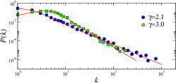
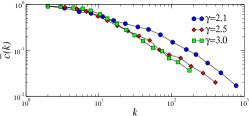
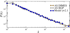
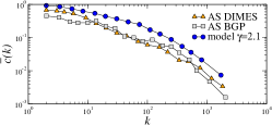
In Figures 1(a) and 1(b) we show, in log-log scale, the degree distribution $P(k)$ and average clustering as a function of the node degree $\bar{c}(k)$ [24], for modeled networks with $N=10000$ and $\bar{k}=6.5$. We observe agreement between simulation results and the analytical prediction for the degree distribution in Equation (4). In Figures 1(c) and 1(d) we compare the same statistics between the modeled networks with $\gamma=2.1$, and the AS Internet topologies from RouteViews BGP tables [25] and DIMES traceroute data [26]. The degree distribution in our networks is remarkably close to the empirical AS degree distribution. The shape of the clustering curve $\bar{c}(k)$ in our networks is similar to the Internet’s. In [27] we also show how clustering can be matched exactly.

(a) Degree distribution $P(k)$.

(b) Average clustering $\bar{c}(k)$.

(c) $P(k)$, Model vs. Internet.

(d) $\bar{c}(k)$, Model vs. Internet.

Figure 1: The first two plots show the degree distribution $P(k)$, and average clustering $\bar{c}(k)$ of $k$-degree nodes. The degree distribution for $\gamma=2.5$ is not shown for clarity. Solid lines in the first plot are the theoretical prediction given by Equation (4). The last two plots show the same statistics for simulated networks with $\gamma=2.1$ vs. AS topologies from RouteViews BGP tables [25] and DIMES traceroute data [26].

III-C Greedy forwarding

We now evaluate the performance of greedy forwarding (GF) strategies on our modeled networks. A node’s address is its hyperbolic coordinates, and each node knows only its own address, the addresses of its neighbors, and the destination address written in the packet. GF forwards a packet at each hop to the neighbor closest to the destination in the hyperbolic space. We present simulation results for two simple forms of GF, original (OGF) and modified (MGF). The OGF algorithm drops the packet if the current hop is a local minimum, meaning that it does not have any neighbor closer to the destination than itself. The MGF algorithm excludes the current hop from any distance comparisons, and finds the neighbor closest to the destination. The packet is dropped only if this neighbor is the same as the packet’s previous hop. We report the following metrics: (i) the percentage of successful paths, $p_{s}$, which is the proportion of paths that reach their destinations; and (ii) the average and maximum stretch of successful paths, denoted by $\bar{s}$ and $\text{max}(s)$ respectively. The stretch is defined as the ratio between the hop-lengths of greedy paths and the corresponding shortest paths in the graph.

We initially focus on static networks, where the network topology does not change, and then emulate network topology dynamics by randomly removing one or more links from the topology. As before, we fix the target number of nodes in the network to $N=10000$ and its average degree to $\bar{k}=6.5$, which roughly matches the Internet’s AS topology. For each generated network, we extract the Giant Connected Component (GCC), and perform GF between $10000$ random source-destination pairs.

(a) Success ratio. (Static networks)

(b) Stretch. (Static networks)

(c) Scenario 1. (Link failures)

(d) Scenario 2. (Link failures)

Figure 2: Performance of greedy forwarding (GF).

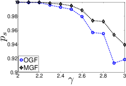
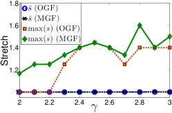
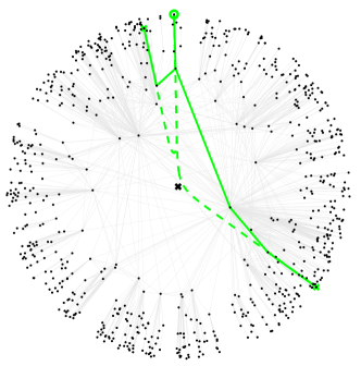
Static networks. Figures 2(a) and 2(b) show the results for static networks of different degree exponent $\gamma$. We see that the success ratio $p_{s}$ increases and the stretch decreases as we decrease $\gamma$ to $2$. For example, for $\gamma=2.1$, i.e., equal to $\gamma$ observed in the AS Internet, OGF and MGF yield $p_{s}=0.99920$ and $p_{s}=0.99986$, with the OGF’s maximum stretch of $1$, meaning that all greedy paths are shortest paths. In summary, GF is exceptionally efficient in static networks, especially for the small $\gamma$’s observed in the vast majority of complex networks [7]. The two GF algorithms yield high success ratios close to $1$ and optimal (or almost optimal) path lengths, i.e., stretch close to $1$. The reason for this remarkable GF performance is the congruency between the network topology and the underlying hyperbolic geometry, as visually demonstrated in Figure 3.

Figure 3: Visualization of a modeled network embedded in the hyperbolic plane, and greedy forwarding in it. The figure shows two hyperbolically straight lines, i.e., geodesics, the dashed curves, vs. the greedy paths, the solid lines, between the same source-destination nodes. The source is the top circled node, and the destinations are marked by crosses. The geodesics and greedy paths are approximately congruent as they follow the same pattern, first going to the disc center, and then veering off towards the destination.

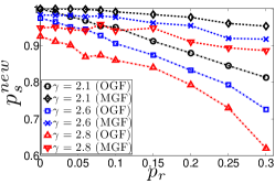
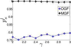
Link failures. We next study the GF performance in dynamic scenarios with link failures. We consider the following two link-failure scenarios. In Scenario 1 we remove a percentage $p_{r}$, ranging from $0\%$ to $30\%$, of all links in the network, recompute the GCC, and compute the new success ratio $p^{new}_{s}$. In Scenario 2, we provide a finer-grain view focusing on paths that used a removed link. We remove one link from the network, recompute the GCC, and find the percentage $p^{l}_{s}$ of successful paths, only among those previously successful paths that traversed the removed link and belong to the new GCC. We repeat the procedure for $1000$ random links, and report the average value for $p^{l}_{s}$. Figures 2(c) and 2(d) present the results. We see that for small $\gamma$’s, the success ratio $p^{new}_{s}$ remains remarkably high, for all meaningful values of $p_{r}$. For example, MGF on networks with $\gamma=2.1$ and $p_{r}\leq 0.1$, yields $p^{new}_{s}>0.99$. Note that the simultaneous failure of $10\%$ of the links in networks like the Internet is a rare catastrophe, but even in this case GF is still efficient. The percentage $p^{l}_{s}$ of MGF paths that used a removed link and that found a by-pass after its removal is also remarkably high, close to $100\%$ for small $\gamma$’s. We do not present the stretch results for brevity. In both scenarios, and for all $\gamma$’s, the average stretch remains remarkably low, below $1.1$.

In summary, GF is not only efficient in static networks, but its efficiency is also remarkably robust with respect to network topology dynamics. Thanks to high path diversity in scale-free networks, there are many shortest paths, disjoint over some links or nodes, between the same source and destination, which all closely follow their geodesics. Link removals affect some shortest paths, but others remain, and greedy forwarding can use the underlying hyperbolic “guidance system” to find them.

Greedy forwarding modifications. Although the success ratios in scale-free networks with small $\gamma$’s are extremely close to $1$, they are not exactly $1$. However, since the performance of our simple GF strategies deteriorates quite slowly with increasing network dynamics, we can expect that simple GF modifications can achieve $100\%$ success ratio and small stretch even in more extreme dynamic network conditions than those we have studied above. We will check our expectations in the next section, in scenarios with random node arrivals and departures.

IV Networks growing in hyperbolic spaces

The model we presented in the previous section generates a whole network at once. However, in many applications, the network topology is formed by nodes gradually arriving over time. In this section, we extend our model for scale-free networks that grow in hyperbolic spaces. We then demonstrate the remarkable efficiency of greedy forwarding in highly dynamic conditions, with nodes randomly arriving and departing the system.

IV-A Growing model

We assume that the network initially consists of $0$ nodes. We number each arriving node by its order of arrival. We do not consider node departures for now. A new node $i\geq 1$ that arrives to the system needs to know: (i) the current number of nodes in the network, including itself, $N(i)=i$; (ii) a system pre-specified parameter $\alpha$ for the node radial density, which as before, will determine the exponent of the degree distribution $\gamma$; and (iii) a system pre-specified constant $c$, which will determine the average node degree as will be explained below. Then, to connect to the network, the node performs the following operations inspired by the model in Section III:

• select an angular coordinate $\theta$ uniformly distributed in $[0,2\pi]$;

• compute the current hyperbolic disk radius $R(i)$ according to $R(i)=\frac{1}{\alpha}\ln\frac{i}{c}$, i.e., $i=ce^{\alpha R(i)}$;

• select a radial coordinate $r\in[0,R(i)]$, according to the probability density function $f(r|R(i))=\frac{\alpha\text{sinh}(\alpha r)}{\text{cosh}(\alpha R(i))-1}\approx\alpha e^{\alpha(r-R(i))}$;

• connect to every node $1\leq j<i$, already in the network, for which the hyperbolic distance to it, denoted by $d_{ij}$, satisfies $d_{ij}\leq R(i)$. 

To build the network in a fully decentralized manner, each arriving node must be able to discover the current number of nodes in it, and the nodes to connect to, i.e. its neighbors. We will present a technique for this later. Before doing so, we analyze the statistical characteristics of the resulting network topologies, and show that they are scale-free.

As before, strong clustering is a direct consequence of the triangle inequality in the hidden space, but we have to show that the node degree distribution follows a power law at any time instance, as soon as the number of nodes in the network is sufficiently large. The analysis becomes more complicated than in Section III, because the hyperbolic disc radius is no longer constant, but grows with the number of nodes in the network.

To proceed, we first compute: (1) the probability density function $f(r,t)$ of the radial coordinate $r$ of a randomly selected node when the number of nodes in the network is some value $t\gg 1$, and (2) the average degree $\bar{k}(r,t)$ of nodes located at distance $r$ from the disc center. Having the expressions for $f(r,t)$ and $\bar{k}(r,t)$ ready, we can then tell how these quantities scale as a function of $r$, and use arguments similar to those in the proof of Theorem 1 to find the degree distribution. The derivation of $f(r,t)$ and $\bar{k}(r,t)$ is in the Appendix. Below we present the final expressions and show that the degree distribution is a power law.

Let $R(t)$ be the hyperbolic disc radius when the number of nodes in the network is $t$. According to the model, $R(t)=\frac{1}{\alpha}\ln\frac{t}{c}$. The approximate expression for the node radial density $f(r,t)$ is:

$$f(r,t)\approx\alpha^{2}(R(t)-r)e^{\alpha(r-R(t))},$$ (5)

leading to:

Lemma 1

For $r<R(t)$ and $t\gg 1$, $f(r,t)\sim e^{\alpha r}$.

For $\alpha>\frac{1}{2}$, the average node degree as a function of $r$ and $t$ is, approximately:

$$\bar{k}(r,t)\approx t\left\{P(r)+\frac{1-e^{-\alpha(R(t)-r)}}{\alpha(R(t)-r)}\left(G(r)-P(r)\right)\right\},$$ (6)

where:

$$G(r)=\left(1-\frac{2\alpha^{2}}{\pi(\alpha-\frac{1}{2})^{2}}+(1-\frac{2\alpha}{\pi(\alpha-\frac{1}{2})})\alpha r\right)e^{-\alpha r}$$

$$+\frac{2\alpha^{2}}{\pi(\alpha-\frac{1}{2})^{2}}e^{-\frac{1}{2}r},$$ (7)

$$P(r)=\frac{2\alpha}{\pi(\alpha-\frac{1}{2})}e^{-\frac{1}{2}r}-\frac{1}{2(\alpha-\frac{1}{2})}e^{-2\alpha\ln\frac{\pi}{2}}e^{-\alpha r},$$ (8)

and the limit $\alpha\to\frac{1}{2}$ is well defined.  The equations above lead to:

Lemma 2

For $\alpha\geq\frac{1}{2}$ and $t\gg 1$, $\bar{k}(r,t)\sim e^{-\frac{1}{2}r}$.

Taken together the two lemmas above result in:

Theorem 2

The described growing model with $\alpha\geq\frac{1}{2}$ produces graphs with a power law node degree distribution $P(k,t)\sim k^{-\gamma}$, where $\gamma=2\alpha+1$.

Proof:

The proof is similar to that of Theorem 1. For $t$ sufficiently large, by Lemma 2, $\bar{k}(r,t)\sim e^{-\frac{1}{2}r}$. Hence, $\bar{r}(k,t)\sim-2\ln k$. By Lemma 1, $f(r,t)\sim e^{\alpha r}$, approximately. Therefore, $P(k,t)\approx f(\bar{r}(k,t),t)|\bar{r}^{\prime}(k,t)|\sim k^{-\gamma}$, with $\gamma=2\alpha+1$. ∎

The average node degree $\bar{k}(t)=\int_{0}^{R(t)}\bar{k}(r,t)f(r,t)dr$ is:

$$\small\bar{k}(t)\approx 2\alpha c\left(e^{(\alpha-\frac{1}{2})R(t)}C_{1}-\alpha R(t)^{2}C_{2}-R(t)C_{3}-C_{4}\right),$$ (9)

where $C_{1}=\frac{2\alpha^{3}}{\pi(\alpha-\frac{1}{2})^{3}(2\alpha-\frac{1}{2})}$, $C_{2}=\frac{2\alpha-\pi(\alpha-\frac{1}{2})}{2\pi(\alpha-\frac{1}{2})}$, $C_{3}=\frac{\alpha}{\pi(\alpha-\frac{1}{2})^{2}}$, $C_{4}=\frac{2}{\pi(\alpha-\frac{1}{2})}\left(\frac{\alpha}{2(\alpha-\frac{1}{2})^{2}}+1\right)$, and the limit $\alpha\to\frac{1}{2}$ is again well defined. Using Equation (9) we can thus choose constant $c$ to set the average node degree to a target value in synthetic networks grown to a target size $t$. For fixed $c$ and $\alpha\to\frac{1}{2}$ the first exponential term in Equation (9) vanishes, and $\bar{k}(t)$ grows very slowly with $t$, as a function of $\ln t$, since $R(t)=\frac{1}{\alpha}\ln\frac{t}{c}$. This property is desirable, as in practical applications, we want the average node degree to depend weakly on the system size. Interestingly, by Theorem 2, $\alpha=\frac{1}{2}$ yields degree exponent $\gamma=2$, which as we have seen in Section III, also maximizes the efficiency of greedy forwarding.

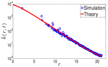
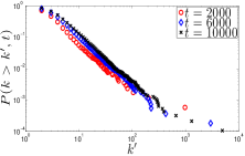
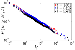
In Figure 4, we check the accuracy of our analytic predictions. The figure is for a synthetic network growing with parameters $\alpha=0.75$, i.e., target $\gamma=2.5$, and $c=0.0014$, i.e., target $\bar{k}(t)=6.5$ when $t=10000$.

(a)	(b)

Figure 4: (a) $\bar{k}(r,t)$ at $t=10000$, and (b) degree ccdf at various $t$.

Figure 4(a) shows, in semi-log scale, that Equation (6) closely matches simulations. Figure 4(b) shows, in log-log scale, the node degree ccdf as the network grows, i.e., at various $t$. The ccdf approximately follows a power law with the slope, i.e., exponent $\gamma-1$,  virtually independent of $t$, as Theorem 2 predicts. The exponent $\gamma$ is approximately $2.5$. We further observe that the ccdf is slightly shifting to the right, indicating that the average node degree in the network grows slowly. At $t=10000$ the average degree is $6.5768$, which is very close to our target value. Similar results hold for other parameter values.

IV-B Decentralized implementation

As mentioned earlier, to build a network in a decentralized manner, each arriving node must be able to discover its neighbors and the current number of nodes in the network. Below we describe an efficient and simple greedy algorithm implementing these tasks. This algorithm is just an example, and other techniques and optimizations are possible.

In a nutshell, the algorithm operates as follows. Each arriving node first contacts a random node currently in the network, which acts as a bootstrap node. The bootstrap node then sends an exploration packet to the network. Each hop that receives the packet writes in it its id and coordinates, as well as the ids and coordinates off all its neighbors, and then forwards the packet to its highest degree neighbor that has not seen the packet before. The process terminates when all neighbors of a node have seen the packet. Below we describe the process in more detail.

The exploration packet starts from the bootstrap node and keeps a list of the node ids it has visited, denoted by $L_{V}$. It also keeps a list of node ids along with their corresponding coordinates, denoted by $L_{C}$. Each node that receives the packet records its own id into $L_{V}$, and its id and coordinates into $L_{C}$. Further, it also records the id and the corresponding coordinates of each of its neighbors into $L_{C}$. The node then selects from its neighbors that are not included in $L_{V}$, the one with the maximum degree, and forwards the packet to it. The process terminates when all neighbors of a node are listed in $L_{V}$, in which case the exploration packet is sent back to the bootstrap node. The list $L_{C}$ is then given to the arriving node.

This process, called search utilizing high degree nodes, is very efficient in power law graphs. In particular, for degree exponents $2<\gamma<3$, the exploration packet can discover a large percentage of nodes in the graph along with their coordinates (recorded in $L_{C}$), by traversing only a small number of hops $\sim N^{2-\frac{4}{\gamma}}$ (recorded in $L_{V}$), see Chapter $13$ in [16]. Having an estimate of the number of nodes, the arriving node can compute the current hyperbolic disc radius, and in turn, its own coordinates. Knowing the hyperbolic disc radius, the coordinates of the nodes, and their ids, it can also compute to which nodes it should connect.

One possible modification of the above basic technique is to impose an upper bound on the size of the $L_{C}$ list. Once such a bound is reached, the current $L_{C}$ list is returned to the bootstrap node, and then cleared in the exploration packet. This extension adds control on the maximum size that the exploration packet can have.

IV-C Greedy forwarding

We now evaluate via simulation the performance of greedy forwarding in highly dynamic conditions, with random node arrivals and departures. Our setup is as follows.

Without loss of generality, time is slotted. During each time slot, a new node arrives w.p. $p=0.1$, and each node currently in the network departs w.p. $q=10^{-5}$. Initially the network consists of $0$ nodes. An arriving node joins the network according to our growing model. It also discovers the current number of nodes in it and their coordinates according to the procedure described earlier. In our experiments below the exploration packet discovers $95\%$ of nodes in the network on average, by traversing only $1.5\%$ of all nodes. If all neighbors of a node depart, the node re-initiates the join process to reconnect to the network. To ensure that the network remains connected, we assume that the first $t_{start}=200$ nodes never depart. According to our growing model, these nodes will have high degrees. High degree nodes are required to maintain connectivity in scale-free graphs [16]. See also the discussion in Section V.

The average number of nodes in the network grows and stabilizes at the steady state value $\bar{t}_{steady}=\frac{p}{q}+t_{start}=10200$.  Note that $\frac{t_{start}}{\bar{t}_{steady}}\approx 2\%$. We set the system parameters to $\alpha=0.5$ and $c=0.01$, which according to our earlier analysis, correspond to the average node degree of $\bar{k}({\bar{t}_{steady})}=6.5$ and degree exponent $\gamma=2$. Recall from Section III that $\gamma=2$ maximizes the efficiency of greedy forwarding, and makes the average degree depend logarithmically on the network size.

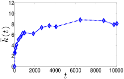
Figure 5(a) shows the average node degree $\bar{k}(t)$ as a function of the current number of nodes $t$ in the network, until and when we reach steady state. The average degree grows initially and then stabilizes above, but close to, our target value of $6.5$.  Figure 5(b) shows the node degree ccdf. The degree exponent is $\gamma\approx 2$, and it does not change as the network grows, as expected.

As mentioned in Section III, we expect simple GF modifications to achieve better performance than our OGF and MGF strategies, even in highly dynamic network conditions. We check these expectations with the Gravity-Pressure Greedy Forwarding algorithm (GPGF) from [9], described below.

Gravity-Presure Greedy Forwarding (GPGF). Each packet carries a bit to indicate whether the packet is in Gravity or Pressure forwarding mode. The packet starts in Gravity mode, where the forwarding procedure is exactly the same as in our OGF algorithm. However, if the packet reaches a local minimum, it is not dropped as in OGF. Instead, it first records the distance of the local minimum to the destination, which we call current local-minimum distance, and then enters Pressure mode. In Pressure mode, the packet maintains a list of the nodes in the network it has visited since it entered this mode, and the number of visits to each node. A node that receives the packet determines all neighbors that the packet has visited the least number of times, selects among those the one with the minimum distance to the destination, and forwards the packet to this neighbor. This process continues until the packet either reaches the destination or a node whose distance to the destination is smaller than the current local-minimum distance. In the latter case, the packet switches back to and continues in the Gravity mode.

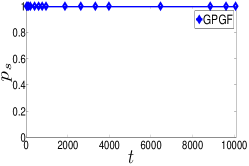
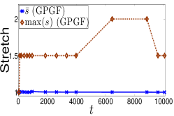
Regardless of underlying space geometry, the success ratio of GPGF is guaranteed to be always $p_{s}=1$ [9], which we confirm in Figure 5(c). What is not guaranteed by the algorithm is the stretch, which can be enormous, as in the worst case a packet can visit all nodes in the network to find its destination. However, in Figure 5(d) we see that GPGF’s stretch is exceptionally low in our networks. In particular, we see that the average stretch $\bar{s}$ remains extremely close to $1$, while the maximum stretch max$(s)$ never exceeds $2$. As before, this remarkable efficiency is due to the congruency between scale-free network topology and underlying hyperbolic geometry, which persists even in highly dynamic conditions.

(a) Average node degree.

(b) Degree ccdf.

(c) Success ratio.

(d) Stretch.

Figure 5: Dynamic networks.

V Discussion

In this section we discuss potential practical applications of our results. One of such applications is overlay network construction [3, 10]. Indeed, the idea of using an underlying geometry to guide the forwarding process is similar in spirit to Distributed Hash Table (DHT) overlay architectures [3]. In overlay networks, messages searching for data content are usually greedily forwarded, based on some distance metric, to the node in the network responsible for the data, usually the node that is closer to the data in terms of the distance metric. The main objective is to have a low average node degree, and a short average hop-length of search paths [3]. Both metrics should grow slowly with the number of nodes in the network $N$. The best efficiency with $O(\ln\ln N)$-long search paths, and $O(1)$ average node degree, can be achieved only in scale-free networks since only in scale-free networks do shortest paths grow as $\sim\ln\ln N$, independently of the average node degree [16]. Therefore, given that greedy paths are approximately shortest in our networks, a property we proved in [28], our results can be used for overlay network construction and routing [10] to improve routing/search efficiency.

However, by no means do we propose a solution which is better than all existing overlay architectures in all aspects. For example, it is often desirable that all nodes in a network have similar degrees, which is not the case with scale-free networks. Another concern may be that while scale-free networks are robust to random node failures/departures, they are vulnerable to failures of the highest degree nodes, resulting in network disconnection [16]. To address this concern, one may consider, for example, hybrid architectures with resilient super-nodes (the high degree nodes) [29], or use techniques similar to those in [30] to ensure recovery when such nodes fail. However, as we have demonstrated in the previous section, it is enough to ensure that high degree nodes corresponding to only $2\%$ of the total steady state number of nodes, do not fail.

Our results also suggest that forwarding information through existing scale-free networks, such as the Internet, should be possible without global topology knowledge and associated routing overhead, which is one of the most serious scaling limitations with the existing Internet architecture [1]. In other words, our results lay the groundwork for potentially moving to an Internet where forwarding can take place without routing.

VI Conclusion

We have shown that scale-free network topologies naturally emerge from, and are congruent with, hyperbolic geometries. This congruency can be used to efficiently guide the forwarding process to find destinations with $100\%$ success probability, following almost optimal shortest paths, even in highly dynamic networks. Our findings complement the important work in [5], and can have several practical applications in overlay network construction for improving routing/search performance.

There are several interesting directions for future work. One is to explore other techniques for decentralized implementation. Another is the design of greedy forwarding strategies that could also be used for improving other network performance metrics, e.g., strategies that could avoid congestion areas, perform load-balancing, and so on.

Finally, our results suggest that forwarding information through existing scale-free networks, e.g., the Internet, should be possible without routing overhead. Therefore, one of the most interesting, yet challenging, future work directions is the following inverse problem: Can we embed any real scale-free network, e.g., the Internet topology, into a hyperbolic space, so that we can greedily forward through this embedding with similar efficiency? How can each node compute its coordinates in the space having no global knowledge of the network topology, so that the resulting embedding is congruent with the space, requiring no coordinate and routing updates even if the network is highly dynamic?

Here we consider a growing network at some time instance where the number of nodes in it is some value $t$, and derive the expressions for the node radial density $f(r,t)$ and the average node degree $\bar{k}(r,t)$. We number each node by its order of arrival. Recall that there are no node departures, and that each node $i\geq 1$ that arrives to the system computes a hyperbolic disc radius $R(i)=\frac{1}{\alpha}\ln\frac{i}{c}$. The radial coordinate $r\in[0,R(i)]$ of node $i$ is distributed according to the density $f(r|R(i))\approx\alpha e^{\alpha(r-R(i))}$.

We start with $f(r,t)$. Let $\{R(1)...R(t)\}$ be the sequence of the hyperbolic disc radii that nodes $\{1...t\}$ compute on their arrival, and let $R$ be the random variable representing the computed disc radius of a randomly selected node from $\{1...t\}$. It is easy to see that for $i\in\{1...t\}$, $P(R\leq R(i))=\frac{i}{t}=\frac{ce^{\alpha R(i)}}{ce^{\alpha R(t)}}=e^{\alpha(R(i)-R(t))}$.

We treat $R$ as a continuous random variable. As we see in Section IV this does not affect the accuracy of the predictions. Therefore, if we denote by $F(R,t)=e^{\alpha(R-R(t))}$ the distribution function of the computed disc radius $R$, then the probability density function of $R$, denoted by $f(R,t)$, is $f(R,t)=\alpha e^{\alpha(R-R(t))}$ and it is obtained by differentiating $F(R,t)$ w.r.t. $R$. Since, given the value of $R$ a node computes its radial coordinate $r$ according to $f(r|R)\approx\alpha e^{\alpha(r-R)}$ and $r\leq R\leq R(t)$, we can write $f(r,t)=\int_{r}^{R(t)}f(r|R)f(R,t)dR$. Performing the integration, we get Equation (5).

We now proceed with $\bar{k}(r,t)$. Its computation is rather long, and we omit it for brevity, see [23]. We can break $\bar{k}(r,t)$ into two parts. The first part $\bar{k}_{init}(r,t)$ is the initial average degree of nodes with radial coordinate $r$, i.e., the average number of nodes already in the network, to which the node connects upon its arrival. The second part $\bar{k}_{new}(r,t)$ is the average number of new connections to nodes at $r$, coming from new nodes arriving to the system after. Clearly, $\bar{k}(r,t)=\bar{k}_{init}(r,t)+\bar{k}_{new}(r,t)$.

We first compute $\bar{k}_{init}(r,t)$. Suppose that the node at $r$ computed a disc radius equal to $R$ when it arrived. According to our model, the node then connected to all other nodes in the network, for which the hyperbolic distance to it was $d\leq R$. The average number of these nodes, denoted by $\bar{k}_{init}(r|R)$, can be computed [23], and its approximate expression for $\alpha\geq\frac{1}{2}$ is $\bar{k}_{init}(r|R)\approx ce^{\alpha R}G(r)$, where $G(r)$ as given by Equation (IV-A).

To obtain $\bar{k}_{init}(r,t)$, we now have to remove the condition on $R$ from $\bar{k}_{init}(r|R)$ by accounting for all possible $R$ with $r\leq R\leq R(t)$. To do so, we need the conditional probability density for $R$, given that a node’s radial coordinate is $r$, denoted by $f(R,t|r)$. Given $f(r|R)$, $f(R,t)$ and $f(r,t)$, we have $f(R,t|r)=\frac{f(r|R)f(R,t)}{f(r,t)}$, and $\bar{k}_{init}(r,t)=\int_{r}^{R(t)}\bar{k}_{init}(r|R)f(R,t|r)dR$.

We now proceed with $\bar{k}_{new}(r,t)$. Let $N_{new}$ be the number of new nodes that arrived to the system after a node with radial coordinate $r$. Clearly, the computed hyperbolic disc radius $R^{\prime}$ of a new such node satisfies $r\leq R^{\prime}\leq R(t)$. According to our model, the new node connects to the node at $r$ only if the hyperbolic distance to it is $d\leq R^{\prime}$. In [23] we show that if $\alpha\geq\frac{1}{2}$ the probability that a new node connects to the node at $r$ is approximately independent of the exact value of $R^{\prime}$ and depends only on $r$. This probability, denoted by $P(r)$, can be easily computed, and is given by Equation (8).

Now, given that the node at $r$ was the $i^{th}$ node arrival, $N_{new}=t-i$. If $\bar{k}_{new}(r,t|i)$ denotes the average number of new connections to node $i$, we can write $\bar{k}_{new}(r,t|i)\approx(t-i)P(r)=(t-ce^{\alpha R(i)})P(r)$. To find $\bar{k}_{new}(r,t)$, we need to remove the condition on the index $i$. In other words, we need to account again for all $R$ with $r\leq R\leq R(t)$. The conditional density of $R$, $f(R,t|r)$, was computed earlier. Therefore, $\bar{k}_{new}(r,t)\approx\int_{r}^{R(t)}(t-ce^{\alpha R})P(r)f(R,t|r)dR$. Adding $\bar{k}_{init}(r,t)$ and $\bar{k}_{new}(r,t)$, and performing the integration, we get $\bar{k}(r,t)$ given by Equation (6).

References

- [1] D. Meyer, L. Zhang, and K. Fall, Eds., RFC4984. The Internet Architecture Board, 2007.
- [2] V. Naumov and T. Gross, “Scalability of routing methods in ad hoc networks,” Performance Evaluation, vol. 62, pp. 193–209, 2005.
- [3] E. K. Lua, J. Crowcroft, M. Pias, R. Sharma, and S. Lim, “A survey and comparison of peer-to-peer overlay network schemes,” IEEE Communications survey and tutorial, vol. 7, no. 2, 2005.
- [4] J. Travers and S. Milgram, “An experimental study of the small world problem,” Sociometry, vol. 32, pp. 425–443, 1969.
- [5] J. Kleinberg, “Navigation in a small world,” Nature, vol. 406, p. 845, 2000.
- [6] M. E. J. Newman, “The structure and function of complex networks,” SIAM Rev, vol. 45, no. 2, pp. 167–256, 2003.
- [7] S. N. Dorogovtsev and J. F. F. Mendes, Evolution of Networks: From Biological Nets to the Internet and WWW. Oxford: Oxford University Press, 2003.
- [8] R. Kleinberg, “Geographic routing using hyperbolic space,” in INFOCOM, 2007.
- [9] A. Cvetkovski and M. Crovella, “Hyperbolic embedding and routing for dynamic graphs,” in INFOCOM, 2009.
- [10] A. Nakao, L. Peterson, and A. Bavier, “Scalable routing overlay networks,” SIGOPS Oper. Syst. Rev., vol. 40, no. 1, 2006.
- [11] J. Kleinberg, “Complex networks and decentralized search algorithms,” in ICM, 2006.
- [12] Y. Shavitt and T. Tankel, “On the curvature of the Internet and its usage for overlay construction and distance estimation,” in INFOCOM, 2004.
- [13] R. Krauthgamer and J. R. Lee, “Algorithms on negatively curved spaces,” in FOCS, 2006.
- [14] I. Abraham, M. Balakrishnan, F. Kuhn, D. Malkhi, V. Ramasubramanian, and K. Talwar, “Reconstructing approximate tree metrics,” in PODC, 2007.
- [15] E. Jonckheere, P. Lohsoonthorn, and F. Bonahon, “Scaled Gromov hyperbolic graphs,” J. Graph Theory, vol. 57, no. 2, 2008.
- [16] S. Bornholdt and H. G. Schuster (Edts.), Handbook of Graph and Networks: From the Genome to the Internet. Berlin: Wiley-VCH, 2002.
- [17] A.-L. Barabási and R. Albert, “Emergence of scaling in random networks,” Science, vol. 286, pp. 509–512, 1999.
- [18] M. R. Bridson and A. Haefliger, Metric Spaces of Non-Positive Curvature. Berlin: Springer-Verlag, 1999.
- [19] M. Girvan and M. E. J. Newman, “Community structure in social and biological networks,” Proc Natl Acad Sci USA, vol. 99, pp. 7821–7826, 2002.
- [20] D. J. Watts, P. S. Dodds, and M. E. J. Newman, “Identity and search in social networks,” Science, vol. 296, pp. 1302–1305, 2002.
- [21] A. Clauset, C. Moore, and M. E. J. Newman, “Hierarchical structure and the prediction of missing links in networks,” Nature, vol. 453, pp. 98–101, 2008.
- [22] M. Gromov, Metric Structures for Riemannian and Non-Riemannian Spaces. Boston: Birkhäuser, 2007.
- [23] F. Papadopoulos, D. Krioukov, M. Boguna, and A. Vahdat, “Greedy forwarding in dynamic scale-free networks embedded in hyperbolic metric spaces,” CAIDA Technical Report number tr-2009-02, 2009, http://www.caida.org/publications/papers/2009/tr-2009-02/.
- [24] D. J. Watts and S. H. Strogatz, “Collective dynamics of “small-world” networks,” Nature, vol. 393, pp. 440–442, 1998.
- [25] “University of Oregon RouteViews Project,” http://www.routeviews.org/.
- [26] “The DIMES project,” http://www.netdimes.org/.
- [27] D. Krioukov, F. Papadopoulos, A. Vahdat, and M. Boguna, “Curvature and temperature of complex networks,” Phys. Rev. E, vol. 80, no. 3, 2009.
- [28] M. Boguñá and D. Krioukov, “Navigating ultrasmall worlds in ultrashort time,” Phys Rev Lett, vol. 102, p. 058701, 2009.
- [29] C. Gkantsidis and M. Mihail, “Hybrid search schemes for unstructured peer-to-peer networks,” in INFOCOM, 2005.
- [30] R. H. Wouhaybi and A. Campbell, “Phenix: supporting resilient low-diameter peer-to-peer topologies,” in INFOCOM, 2004.