Transition redshift: new kinematic constraints from supernovae
Abstract
The transition redshift (deceleration/acceleration) is discussed by expanding the deceleration parameter to first order around its present value. A detailed study is carried out by considering two different parameterizations: and , and the associated free parameters () are constrained by 3 different supernova samples. The previous analysis by Riess et al. [ApJ 607, 665, 2004] using the first expansion is slightly improved and confirmed in light of their recent data (Gold07 sample). However, by fitting the model with the Supernova Legacy Survey (SNLS) type Ia sample we find that the best fit to the redshift transition is instead of as derived by the High-z Supernovae Search (HZSNS) team. This result based in the SNLS sample is also in good agreement with the Davis et al. sample, (). Such results are in line with some independent analyzes and accommodates more easily the concordance flat model (CDM). For both parameterizations, the three SNe type Ia samples considered favor recent acceleration and past deceleration with a high degree of statistical confidence level. All the kinematic results presented here depend neither on the validity of general relativity nor the matter-energy contents of the Universe.
1 INTRODUCTION
It is now widely believed that the universe at redshifts smaller than unity underwent a “dynamic phase transition” from decelerating to accelerating expansion which has been corroborated by several independent analyzes. In the context of the general relativity theory such a phenomenon can be interpreted as a dynamic influence of some sort of dark energy whose main effect is to change the sign of the universal decelerating parameter .
The most direct observation supporting the present accelerating stage of the Universe comes from the luminosity distance versus redshift relation measurements using supernovae (SNe) type Ia (Riess et al. 1998; Perlmutter et al. 1999; Riess et al. 2004, 2007; Astier et al. 2006; Wood-Vasey et al. 2007; Davis et al. 2007; Kowalski M., et al. 2008) initially interpreted in light of CDM scenarios using either background or inhomogeneous luminosity distances (Santos et al. 2008; Santos & Lima 2008). However, independent theoretical observational analyzes points to more general models whose basic ingredient is a negative-pressure dark energy component (for review see, Padmanabhan 2003; Peebles & Ratra 2003; Lima 2004; Copeland et al. 2006).
The convergence of many high-quality experimental results are now strongly suggesting that the cosmic picture at present is the following: the spatial geometry (curvature) is flat, or more approximately flat, and the dynamics is governed by a component called dark energy, 3/4 of composition, and 1/4 for matter component (baryons plus dark). Among a number of possibilities to describe this dark energy component, the simplest and most theoretically appealing way is by means of a positive cosmological constant . Others possible candidates are: a vacuum decaying energy density, or a time varying -term (Ozer & Taha 1987; Freese et al. 1987; Carvalho et al. 1992; Lima & Maia 1993; 1994; Maia & Lima 1999; 2002; Lima 1996; Overduin & Cooperstock 1998; Cunha et al. 2002a,b; Cunha & Santos 2004; Alcaniz & Lima 2005; Carneiro & Lima 2005; Fabris et al. 2007), a time varying relic scalar field slowly rolling down its potential (Ratra & Peebles 1988; Frieman et al. 1995; Caldwell et al. 1998; Saini et al. 2000; Caldwell 2000; Carvalho et al. 2006), the so-called “X-matter”, an extra component simply characterized by an equation of state (Turner & White 1997; Chiba et al. 1997; Alcaniz & Lima 1999, 2001; Kujat et al. 2002; Alcaniz et al. 2003), the Chaplygin gas whose equation of state is given by where is a positive constant (Kamenshchik et al. 2001; Bento et al. 2002; Dev et al. 2003; Bento et al. 2003; Cunha et al. 2004; Lima et al. 2006a,b), among others (Lima & Alcaniz 1999; Chimento et al. 2001; Freese & Lewis 2002; Pavon & Zimdahl 2005). For SFC and XCDM scenarios, the parameter may be a function of the redshift (see, for example, Efstathiou 1999; Cunha et al. 2007), or still, as it has been recently discussed, it may violate the dominant energy condition and assume values when the extra component is named phantom cosmology (Caldwell 2002; Lima et al. 2003; Perivolaropoulos 2005; Gonzalez-Diaz & Siguenza 2004; Lima & Alcaniz 2004; Santos & Lima 2008). It should be stressed, however, that all these models are based on the validity of general relativity or some of its scalar-tensorial generalizations.
On the other hand, Turner & Riess (2002) have discussed an alternative route - sometimes called kinematic approach - in order to obtain information about the beginning of the present accelerating stage of the Universe with no assumption concerning the validity of general relativity or even of any particular metric gravitational theory (in this connection see also Weinberg 1972). Although considering that such a method does not shed light on the physical or geometrical properties of the new energetic component causing the acceleration it allows one to assess the direct empirical evidence for the transition from decelerating to accelerating in the past as provided by SNe type Ia measurements. In their preliminary analysis it was found that the SNe data favor recent acceleration () and past deceleration ().
More recently, with basis on the same approach, the High-z Supernova Search (HZSNS) team have obtained at c.l. (Riess et al. 2004) which has been further improved to () c.l. (Riess et al. 2007). Many authors have used these values of the transition redshift for imposing constraints on the cosmic parameters as an independent and trustworth discriminator for cosmology (Gardner 2005; Virey et al. 2005; Qiang & Zhang 2006; Gong & Wang 2006; Gong & Wang 2007, Xu et al. 2007; Ishida et al. 2008).
In this article, we constrain the transition redshift by expanding the deceleration parameter around its present value. A detailed analysis is carried out for 2 different parameterizations: and . We show that the kinematic analysis based on the SNLS (Astier et al. 2006), as well as the one recently compiled by Davis et al. 2007, yield a transition redshift () in better agreement with the flat CDM model () than the one provided by Riess et al. (2007) using the High-z Supernova Search (HZSNS) sample.
2 KINEMATIC APPROACH AND ANALYSIS
To begin with, let us assume that the Universe is spatially flat as motivated by inflation and the WMAP results (Spergel et al. 2007, Komatsu et al. 2008). Following Turner & Riess (2002) and Riess et al. (2004), the luminosity distance is defined by the following integral expression (with )
| (1) |
where the is the Hubble parameter, and, , the deceleration parameter, is defined by
| (2) |
Although generalizable for non-zero curvature, Eq. (1) is not a crude approximation as one may think at first sight. In the framework of a flat FRW type universe, it is an exact expression for the luminosity distance which depends on the expressions of the present Hubble constant, , and the epoch-dependent deceleration parameter, . The simplest way to work with the coupled definitions (1) and (2) as a kinematic model for the SN type Ia data is by adopting a parametric representations for . As one may check, in the case of a linear two-parameter expansion for (Riess et al. 2004), the integral (1) can be represented in terms of a special function as (see Appendix A)
| (3) | |||||
where is the present value of the deceleration parameter, is the derivative in the redshift evaluated at , and is the incomplete gamma function (see, Abramowitz & Stegun 1972) with the condition must be satisfied (more details in the Appendix). By using the above expressions we may get information about , and, therefore, about the global behavior of . Note also that a positive transition redshift, , may be obtained only for positive signs of (the variation rate of ) since is negative and the dynamic transition (from decelerating to accelerating) happens at , or equivalently, .
Another parametrization of considerable interest is (Xu et al. 2007). It has the advantage to be well behaved at high redshift while the linear approach diverges at the distant past. In this case we can write the integral (1) as (see Appendix A)
| (4) | |||||
where is the present value of the deceleration parameter, is the parameter yielding the total correction in the distant past (). Note also that a positive transition redshift, , may be obtained only for positive signs of since is negative and the dynamic transition (from decelerating to accelerating) happens at , or equivalently, .
The so-called Gold07 sample from the HZSNS team is a selection of 182 SNe Ia events distributed over the redshift interval , and constitutes the compilation of the best observations made so far by them which were completed by 16 events from the Supernova Cosmology Project observed with the Hubble Space Telescope (HST).
The current data from SNLS collaboration correspond to the first year results of its planned five year survey. The total sample includes 71 high- SNe Ia in the redshift range plus 44 low- SNe Ia. This data set is arguably (due to multi-band, rolling search technique and careful calibration) the best high- SNe Ia compilation to date, as indicated by the very tight scatter around the best fit in the Hubble diagram and a careful estimate of systematic uncertainties. Another important aspect to be emphasized on the SNLS data is that they seem to be in a better agreement with WMAP 3-years results (Spergel et al. 2007) than the previous Gold04 sample observed by Riess et al. (2004). For a more detailed discussion see e.g., Jassal et al. 2006.
For completeness, we also consider the Type Ia Supernovae compilation by Davis et al. 2007. This extended sample is formed by 192 SNIa consisting of 45 SNe from a nearby SNe Ia subsample, plus 57 from SNLS and 60 intermediate redshift SNe from ESSENCE (Wood-Vasey et al. 2007), and, finally, 30 high redshift Gold07 SNe with internally consistent magnitude offsets. The supernovae span the redshift range (Riess et al. 2007).
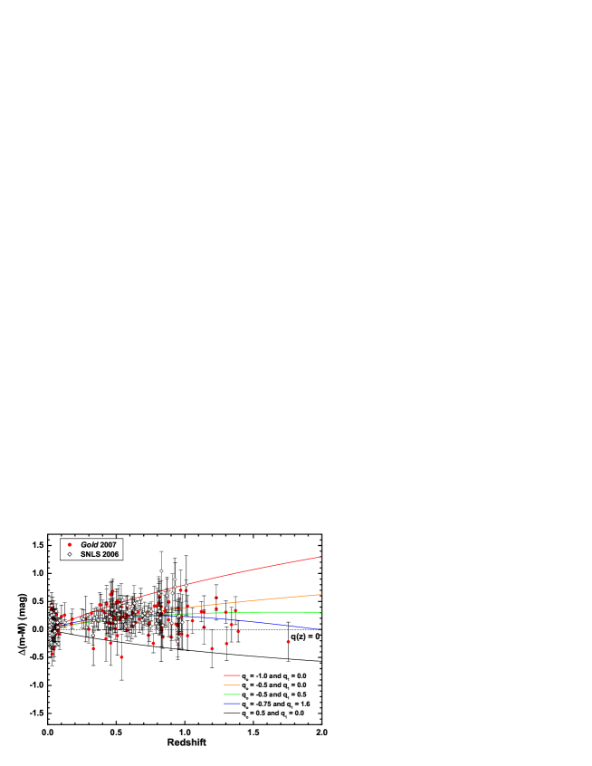
In figure 1 we show the theoretical predictions of the kinematic approach to the residual Hubble diagram with respect to an eternally coasting Universe model (). Such a diagram is usually presented in terms of the bolometric distance modulus which is defined by (Peebles 1993). The different models are characterized by the selected values of and , as depicted in the diagram. The SNe type Ia data shown in the panel comprise both the SNLS (Astier et al. 2006) and HZSNS (Riess et al. 2007) samples as indicated. At this point, it is natural to ask about the likelihood contours in the plane () and the probability of the transition redshift derived for each sample separately, as well as to the whole set of data.
In order to obtain that, let us consider the maximum likelihood that can be determined from a statistics for a given set of parameters
| (5) |
where is the uncertainty in the individual distance moduli, is the dispersion in SNe redshifts due to peculiar velocities (Riess et al. 2004, 2007), and the complete set of parameters is .
In what follows we investigate the bounds arising on the empirical parameters and the probability of the redshift transition for each SNe type Ia sample. By marginalizing the likelihood function over the nuisance parameter, , the contours and the probabilities of the transition redshift for each sample are readily computed.
2.1 Gold Sample Analysis:
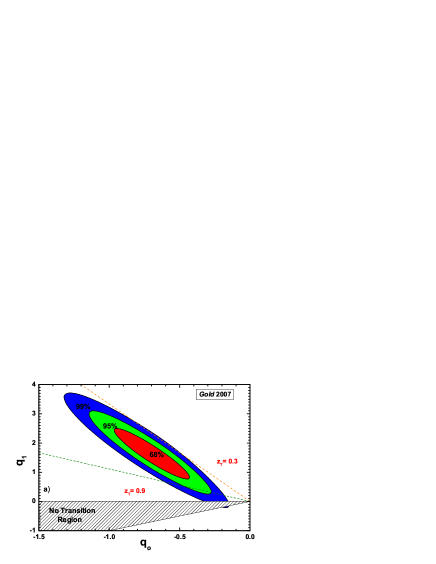
In figure 2a we show the plane for confidence levels of , and for the Gold07 sample. Note that it strongly favors a Universe with recent acceleration () and previous deceleration (). With one free parameter the confidence region is and with () confidence level. It should be remarked the presence of a forbidden region forming a trapezium. The horizontal line in the top is defined by which leads to an infinite (positive or negative) transition redshift while the segment at is the infinite future (). Actually, since , in the infinite future () one finds that . In addition, the values of associated with the horizontal segment in the bottom are always smaller than -1 (therefore, after the infinite future!) since . Finally, one may conclude that the vertical segment is associated with , thereby demonstrating that the hachured trapezium is actually a physically forbidden region.
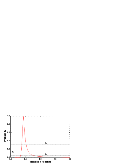
In Figure 2b, one may see the probability of the associated transition redshift defined by . It has been derived by summing the probability density in the versus the plane along lines of constant transition redshift, . The resulting analysis yields () () for one free parameter which is in reasonable agreement with the value quoted by Riess et al. (2004). In our analysis, the asymmetry in the probability of is produced by a partially parabolic curve obtained when is minimized. It is clear that the central value () does not agree with several dynamical flat models in % and % confidence level. In particular, in the flat CDM concordance model ().
2.2 Gold Sample:
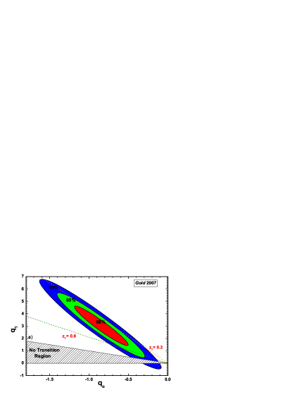
In figure 3a we show the plane for confidence levels of , and using the Gold07 sample for the above phenomenological law. Again, we see that a Universe with recent acceleration () and previous deceleration () is strongly favored. With one free parameter the allowed region is and with () confidence level. Note also the presence of a physically forbidden region forming a trapezium (cf Fig. 2a). As one may check, the horizontal line at the bottom is defined by which leads to a transition redshift in the infinite future () while the segment also defines an extreme line of transition redshifts. Note also that all transition redshifts associated with the vertical segment of the triangle (on the axis defined by ) take values on the future, more precisely, on the interval [-1,-1/2].
In Figure 3b we display the probability of the transition redshift which is defined by . The resulting analysis yields () () for one free parameter. This central value agrees with the flat concordance model only at % (). Note that the straight lines denoting (transition redshift for a flat CDM with ) and (for a CDM with and ) are outside of the regions in both parametrizations (see Figs. 2a and 3a).
2.3 Analysis from SNLS:
Let us now consider the Astier et al. 2006 data sample to constrain the plane for the above linear phenomenological description.
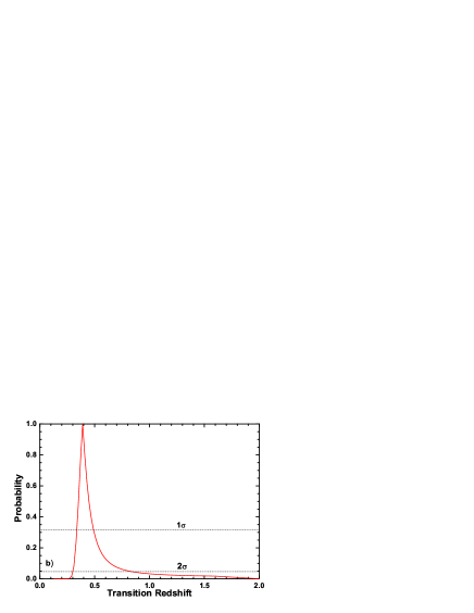
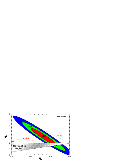
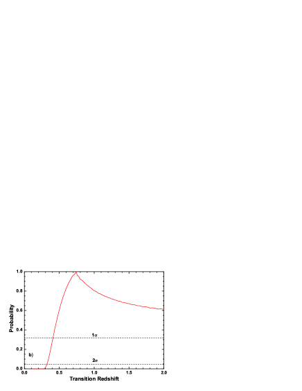
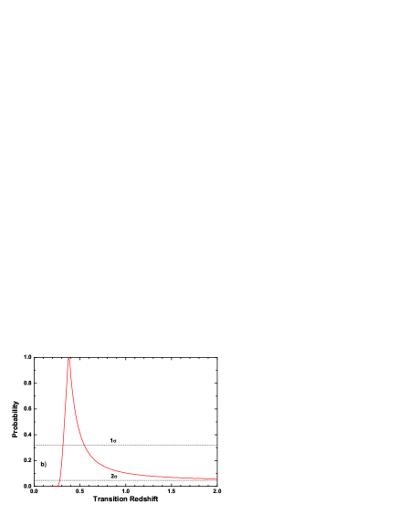
In figure 4a we show the plane with confidence levels of , and to the SNLS data set. With one free parameter the confidence region is and with (). In the panel we see that is only marginally compatible at 3 while is well inside with reasonable confidence (2). Probably, this apparent conflict comes from the fact that there are few data with high dispersions in (see commentary by Astier et al. in their paper). Interestingly, the forbidden region now crosses the confidence level curves (even at 1), however, the SNLS data (different from the Gold07 sample data) are compatible with the existence of a transition redshifts in the future, that is, beyond the forbidden region (). In particular, such a result reinforces the interest to examine higher order corrections (beyond the first order expansion) within the kinematic approach.
In figure 4b we show the likelihood function for the transition redshift. Our analysis furnishes the best fit () for one free parameter. The likelihood is not well behaved at high redshifts because its upper limit is not known. Actually, although supplying an excellent adjustment when combined with the WMAP 3-years and cosmic concordance model, the superior limit of is not tightly constrained by the present SNLS sample. This poor inference should be expected from the very beginning in virtue of the absence of data for in the SNLS sample.
2.4 SNLS:
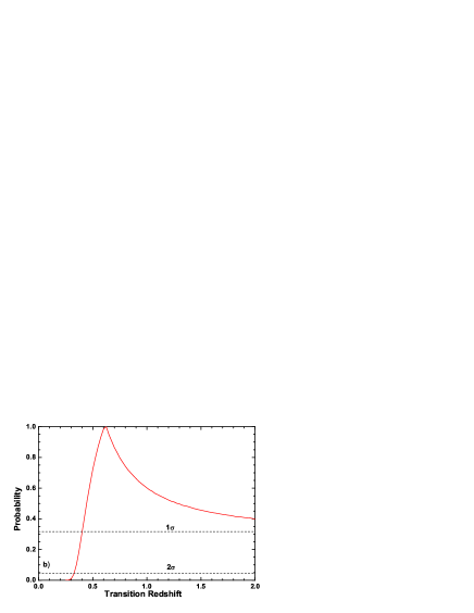
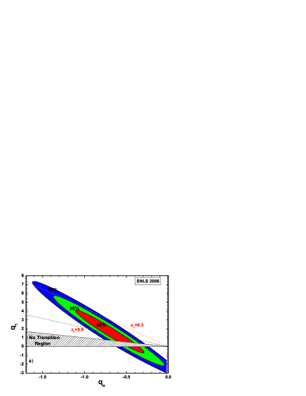
In figure 5a we show the plane to the SNLS data set in the context of the above quoted parameterization. The allowed regions at , and are indicated. With one free parameter the confidence region is and with (). In the panel we see that (flat CDM with ) is outside of the allowed (2) region while (flat CDM with and ) is well inside.
It is worth noticing that the forbidden region is now represented by a right-angle triangle. Interestingly, it crosses the confidence level curves (even at 1), however, the SNLS data (different from the Gold07 sample data) are compatible with the existence of a transition redshifts in the future, that is, for negative value of . In particular, such a result reinforces the interest to examine higher order corrections (beyond the first order expansion) within the kinematic approach. In particular, this means that some theoretical problems associated with the existence of horizons in the future of models that accelerates forever must be solved in a natural way (see, for instance, Carvalho et al. (2006)).
In figure 5b we show the likelihood function of the transition redshift. Our analysis furnishes the best fit with inferior value () for one free parameter and the upper value to is too high. Actually, it is very high and completely incompatible with observations (see also Fig. 4b). Such a poor inference at high from SNLS sample (Astier et al. 2006) for both parameterizations should be expected because the absence of data for . This is calling our attention to the importance of observing high redshift supernovae within the SNLS collaboration.
2.5 Davis 2007 Sample:
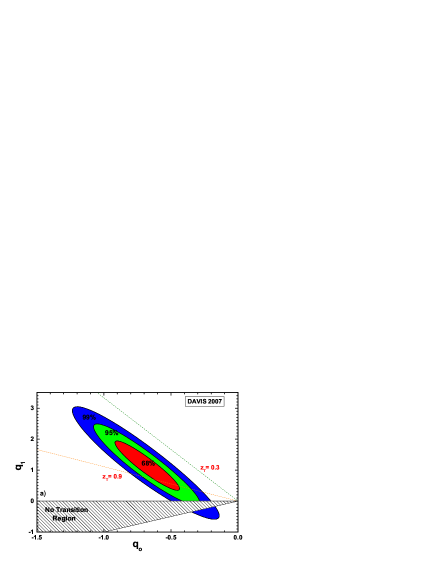
Let us now discuss the constraints within the linear approach for the Davis et al. data set. In figure 6a we display the plane for confidence levels of , and as indicated. Note that such a sample also favors a Universe with recent acceleration () and previous deceleration (). With one free parameter the confidence region is and with (). In the same panel we also see that is completely outside even of the significant region while is well inside with high confidence.
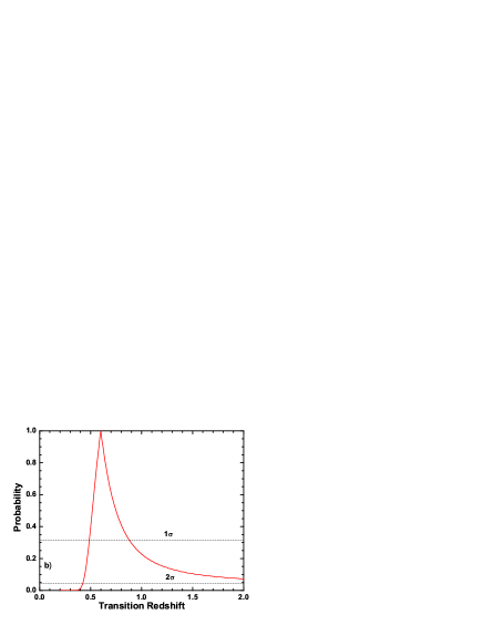
In figure 6b we show the likelihood function for the transition redshift. We can see that () for one free parameter. These results are in better accord with flat LCDM models. Such a fact may be somewhat related to the higher degree of statistical completeness obtained when the SNe type Ia samples are added.
2.6 Davis 2007 Sample:
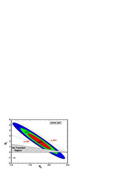
In Figure 7a we display the plane when Davis sample is considered for parameterization. With one free parameter the confidence region is and with (). In the same panel we also see that is outside while is well inside with high confidence.
In figure 7b we show the likelihood function of the transition redshift. We can see that () for one free parameter. This results is comparable with the constraints from the Gold07 sample for the same parameterization (see subsection 2.2). It is also interesting that the Davis et al. sample also suggests (for both parameterizations) the existence of a transition redshift in the future (). Such a possibility it will be discussed with more detail in a forthcoming communication (Lima and Cunha 2008).
3 RECONSTRUCTING THE DECELERATING PARAMETER
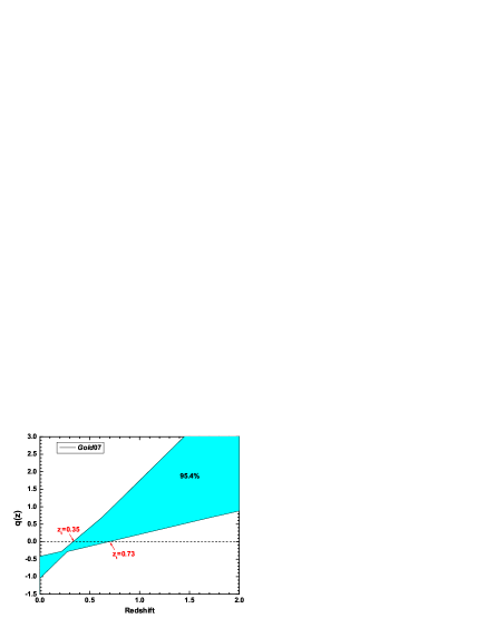
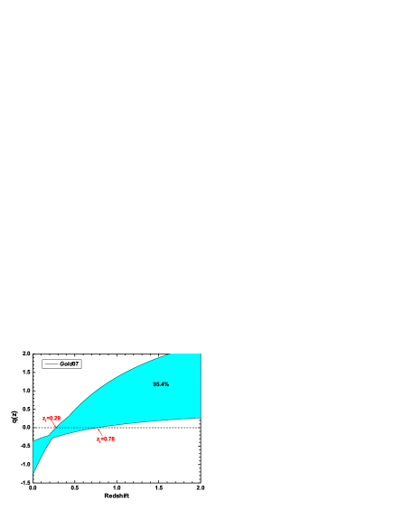
At this point it is interesting to investigate how a joint analysis constrains the redshift evolution of the decelerating parameter. However, since the time evolutions are quite similar for the different parameterizations, in what follows we focus our attention on the Gold07 sample. The basic results are displayed in Figures 8a and 8b.
In Figs. 8a we see the evolution of the decelerating parameter as a function of the redshift for the parameterization . The shadow denotes the 2 region.
In Fig 8b the evolution is shown for a two-parameter expansion history driven by . For both cases, we also show the lower and upper values () of the transition redshifts which is defined by the condition (). Note also that for both parameterizations the data favor the recent acceleration () and past deceleration () with high confidence level.
In Table 1 we summarize the basic constraints on the transition redshift () established in the present work. As shown there, for a given phenomenological law the limits were derived separately for each sample of SNe type Ia data.
4 CONCLUSION
The most remarkable dynamical feature distinguishing dark energy and matter dominated models is the present accelerating stage. However, the observed structures must be formed in a past decelerated phase dominated by matter. This leads naturally to a dynamic phase transition from decelerating to accelerating in the course of the Universe’s evolution. This is the most natural scenario within the framework of the general relativity. It has been confirmed by several disparate observations ranging from the anisotropy of the CMB, SNe Ia, galaxy clusters, age of the universe, however, even considering the high-quality of the present data the whole set is still compatible with many different dark energy models.
The basic information about the deceleration parameter has been obtained here through a model independent analysis using two different phenomenological laws, namely: , as proposed by Riess et al. (2004) and (Xu et al. 2007). The contours to the plane () and the likelihood function for transition redshift were discussed in detail with basis on the data sample by Riess et al. (2007), Astier et al. (2006) and Davis et al. (2007). In order to compare the predictions, we have presented the analysis first for each sample separately. As we have seen, although considering the presence of no transition regions (see Figs. 2a, 3a, 4a, 5a, 6a and 7a), both sample strongly favor a Universe with recent acceleration () and previous deceleration ().
The likelihood function for the transition redshift is more well defined for the Riess et al. (2007) and Davis et al. (2007) data. In table 1 we summarize the main results related to the transition redshift in the present kinematic approach. For both samples, our analysis provides a model independent evidence that a dynamic phase transition from decelerating to accelerating happened at redshifts smaller than unity. Hopefully, the constraints on will be considerably improved in the near future with the increasing of supernovae data at intermediate and high redshifts.
| Sample | Best fit | Confidence region () |
|---|---|---|
| Riess07………. | ||
| Astier06……… | ||
| Davis07……… | ||
| Riess07………. | ||
| Astier06……… | high | |
| Davis07……… |
Acknowledgments
The authors are grateful to R. C. Santos, L. Marassi and S. Vitenti for helpful discussions. This work was partially supported by the CNPq - Brazil and FAPESP. JASL is grateful to FAPESP grant No. 04/13668 and JVC is supported by FAPESP No. 05/02809-5.
References
- Abramow (1972) Abramowitz M. & Stegun I. A., 1972, Handbook of Mathematical Functions. Dover Publications
- alcaniz1 (1999) Alcaniz J. S. & Lima J. A. S. 1999, ApJ, 521, L87, [astro-ph/9902298]
- alcaniz1 (2001) Alcaniz J. S. & Lima J. A. S., 2001, ApJ, 550, L133, [astro-ph/0101544]
- alcaniz2 (2003) Alcaniz J. S., Lima J. A. S. & Cunha J. V., 2003, Mon. Not. Roy. Astron. Soc., 340, L39, [astro-ph/0301226]
- alcaniz4 (2005) Alcaniz J. S. & Lima J. A. S., 2005, Phys. Rev. D, 72, 063516, [astro-ph/0507372]
- Bent1 (2006) Astier P. et al., 2006, Astron. Astrophys., 447, 31
- Bent1 (2002) Bento M. C., Bertolami O. & Sen A. A., 2002, Phys. Rev. D, 66, 043507
- Bent2 (2003) Bento M. C., Bertolami O. & Sen A. A., 2003, Phys. Rev. D, 67, 063003
- Cald1 (1998) Caldwell R. R., Dave R. & Steinhardt P. J., 1998, Phys. Rev. Lett., 80, 1582
- Cald2 (2000) Caldwell R. R., 2000, Braz. J. Phys., 30, 215
- Cald3 (2002) Caldwell R. R., 2002, Phys. Lett. B, 545, 23
- CL205 (2005) Carneiro, S. & Lima J. A. S., 2005, Int. J. Mod. Phys. A, 20, 2465, [gr-qc/0405141]
- carv (1992) Carvalho J. C., Lima J. A. S. & Waga I., 1992, Phys. Rev. D, 46, 2404
- carv (1992) Carvalho F. C. et al., 2006, Phys. Rev. Lett. 97, 081301, [astro-ph/0608439]
- chiba (1997) Chiba T., Sugiyama N., and Nakamura T., 1997, MNRAS, 289, L5
- Chim (2001) Chimento L. P., Jakubi A. S. & Zuccala N. A., 2001, Phys. Rev. D, 63, 103508
- Copeland (2006) Copeland E. J., Sami M. & Tsujikawa S., 2006, IJMPD, 15, 1753
- cunha02 (2002) Cunha J. V., Lima J. A. S. & Alcaniz J. S., 2002a, Phys. Rev. D, 66, 023520, [astro-ph/0202260]
- cunha02b (2002) Cunha J. V., Lima J. A. S. & Pires N., 2002b, Astron. & Astrophys., 390, 809, [astro-ph/0202217]
- cunha04a (2004) Cunha J. V. & Santos R. C., 2004, Int. J. Mod. Phys. D, 13, 1321, [astro-ph/0402169]
- cunha04b (2004) Cunha J. V., Alcaniz J. S. & Lima J. A. S., 2004, Phys. Rev. D, 69, 083501, [astro-ph/0306319]
- cunha07 (2007) Cunha J. V., Marassi L. & Santos R. C., 2007, Int. J. Mod. Phys. D, 6, 403, [astro-ph/0608686]
- Davis07 (2007) Davis T. M., Mörtsell E., Sollerman J. et al., 2007, ApJ, 666, 716
- Dev (1995) Dev A., Jain D. & Alcaniz J. S., 2003, Phys. Rev. D, 67, 023515
- Efst (1999) Efstathiou G., 1999, Mon. Not. Roy. Astron. Soc., 310, 842
- Fabris07 (2007) Fabris J. C., Shapiro I. L. & Sola J., 2007, J. Cosmol. Astropart. Phys., 0702, 016
- Free1 (1987) Freese K. et al., 1987, Nucl. Phys. B, 287, 797
- Free2 (2002) Freese K. & Lewis M., 2002, Phys. Lett. B, 540, 1
- Fr95 (1995) Frieman J. A. et al., 1995, Phys. Rev. Lett., 75, 2077
- Gard (2005) Gardner C. L., 2005, Nucl. Phys. B, 707, 278
- Gong (2006) Gong Y. & Wang A., 2006, Phys. Rev. D, 73, 083506
- Gong (2007) Gong Y. & Wang A., 2007, Phys. Rev. D, 75, 043520
- Gon04 (2004) Gonzalez-Diaz P. F. & Siguenza C. L., 2004, Nucl. Phys. B, 697, 363
- Ishida08 (2008) Ishida E. E. O., Reis R. R. R., Toribio A. V. & Waga I., 2008, Astropart. Phys., 28, 547
- Komatsu2008 (2001) Komatsu E. et al., 2008 (ArXiv: 0803.0547v1)
- Ozer (2001) Kamenshchik A., Moschella U. & Pasquier V., 2001, Phys. Lett. B, 511, 265
- perm1 (2008) Kowalski M., et al., 2008 (ArXiv:08044142v1)
- kujat (2002) Kujat J., Linn A. M., Scherrer R. J., Weinberg D. H., 2002, ApJ, 572, 1
- Jassal (2006) Jassal H. K., Bagla J. S. & Padmanabhan T., 2006 (astro-ph/0601389)
- LimaMaia99 (2006) Lima J. A. S. & Maia J. M. F., 1993, Mod. Phys. Lett. A, 8, 591
- LimaMaia94 (2006) Lima J. A. S. & Maia J. M. F., 1994, Phys. Rev. D, 49, 5597
- Lima (1996) Lima J. A. S., 1996, Phys. Rev. D, 54, 2571, [gr-qc/9605055]
- Lima1 (1999) Lima J. A. S. & Alcaniz J. S., 1999, Astron. Astrophys, 348, 1, [astro-ph/9902337]
- LimCunAl03 (2003) Lima J. A. S., Cunha J. V. & Alcaniz J. S. 2003, Phys. Rev. D, 68, 023510, [astro-ph/0303388]
- Lima (2004) Lima J. A. S., 2004, Braz. J. Phys., 34, 194, [astro-ph/0402109]
- LimaAlc04 (2004) Lima J. A. S. & Alcaniz J. S., 2004, Phys. Lett. B, 600, 191, [astro-ph/0402265]
- LimCunAl06 (2006) Lima J. A. S., Cunha J. V. & Alcaniz J. S. 2006a, [astro-ph/0608469]
- LimCunAl06b (2006) Lima J. A. S., Cunha J. V. & Alcaniz J. S. 2006b, [astro-ph/0611007]
- MaiaLima99 (2006) Maia J. M. F. & Lima J. A. S., 1999, Phys. Rev. D, 60, 101301, [astro-ph/9910568]
- MaiaLima02 (2006) Maia J. M. F. & Lima J. A. S., 2002, Phys. Rev. D, 65, 083513, [astro-ph/0112091]
- OvCo (1998) Overduin F. M. & Cooperstock F. I., 1998, Phys. Rev. D, 58, 043506
- Ozer (1987) Ozer M. & Taha O., 1987, Nucl. Phys. B, 287, 797
- Padman (2003) Padmanabhan T., 2003, Phys. Rep., 380, 235
- Pavon (2003) Pavon D. & Zimdahl W., 2005, Phys. Lett. B628, 206
- Peebles (2003) Peebles P. J. E., 1993, Principles of Physical Cosmology, Princeton UP, New Jersey
- Peebles (2003) Peebles P. J. E. & Ratra B., 2003, Rev. Mod. Phys., 75, 559
- Perivo05 (2005) Perivolaropoulos L., 2005, Phys. Rev. D, 71, 063503
- perm1 (1999) Perlmutter S., et al., 1999, ApJ, 517, 565
- Qiang (2006) Qiang Y. & Zhang T.-J., 2006, Mod. Phys. Lett. A, 21, 75
- ratra (1988) Ratra B. & Peebles P. J. E., 1988, Phys. Rev. D, 37, 3406
- riess (1998) Riess A. G. et al., 1998, AJ, 116, 1009
- riess (2004) Riess A. G. et al., 2004, ApJ, 607, 665
- riess (2007) Riess A. G. et al., 2007, ApJ, 659, 98
- Sain (2000) Saini T. D. et al., 2000, Phys. Rev. Lett., 85, 1162
- Santos (2008) Santos R. C., Cunha J. V. & Lima J. A. S., 2008, Phys. Rev. D 77, 023519, arXiv:0709.3679 [astro-ph]
- Santos (2008) Santos R. C. & Lima, J. A. S., 2008, Phys. Rev. D 77, 083505, arXiv:0803.1865 [astro-ph]
- Sain (2000) Spergel D. N. et al., 2007, ApJ, 170, 377
- turner (1997) Turner M. S. & White M., 1997, Phys. Rev. D, 56, R4439
- turner (2002) Turner M. S. & Riess A. G., 2002, ApJ, 569, 18
- Virey (2005) Virey J.-M. et al., 2005, Phys. Rev. D, 72, R061302
- Weinberg (1972) Weinberg S., 1972, Cosmology and Gravitation, John Wiley Sons, N.Y.
- Wood-Vasey07 (2007) Wood-Vasey W. M., Miknaitis G., Stubbs C. W., 2007, ApJ, 666, 694
- Xu (2007) Xu L., Zhang C., Chang B. & Liu H., 2007 (astro-ph/0701519)
Appendix
Appendix A Distance Luminosity in the Kinematic Description
In this Appendix, we shall outline the method used to obtain the theoretical expression for when the kinematic approach is based on the expansion: . The result is valid for a geometrically flat model. By definition:
| (A1) |
where we have set and H is the Hubble parameter which in the kinematic approach must be obtained in terms of the decelerating parameter:
| (A2) |
By integrating the above equation and inserting the result into (A1) it follows that
| (A3) |
which is just (2). Replacing the expansion of , we obtain
| (A4) |
where and . Now, a simple variable change results
| (A5) | |||||
where is the incomplete gamma function (Abramowitz & Stegun 1972).
Interestingly, in the linear approximation the luminosity distance can also be directly written in terms of the transition redshift:
| (A6) |
For the second parametrization , we obtain
| (A7) |
where and . As well as in the last integral, a simple variable change results
| (A8) | |||||
Or yet, in terms of the transition redshift:
| (A9) |