On Scalar and Vector Potentials for the Nonlinear
Electromagnetic Forces

retired from: Max-Planck-Institut für Plasmaphysik, Garching, Germany

Abstract

The potential concept that is successful in classical electrodynamics should also be applicable to the nonlinear electromagnetic forces acting on matter. The obvious method of determining these potentials should be provided by Helmholtz’s theorem. It is found, however, that the theorem fails in most practical instances. Other methods to find the potentials – as pursued in plasma physics – are examined and found to yield functions which depend on the chosen coordinate system. Thus they cannot be considered as invariant potentials from which physical forces may be derived. Practical consequences of these mathematical findings are discussed.

Keywords

1. Lorentz force

2. Maxwell’s equations

3. Helmholtz’s theorem

4. magnetized plasmas

5. ideal and resistive magnetohydrodynamics

6. magnetic plasma confinement

P.A.C.S.: 41.20.Cv, 41.20.Gz, 45.20.da, 47.65.-d, 52.25.Xz, 52.30.Cv, 52.55.-s, 52.65.Kj

1 Introduction

In classical electrodynamics the force density acting on a volume element, which carries charge and current, is derived from the divergence of Maxwell’s stress tensor. We have the well known result [1] which may also be derived directly from the Lorentz force:

$$\vec{F}=\rho\;\vec{E}+\vec{j}\times\vec{B}$$ (1)

Both the electric and the magnetic force are nonlinear, since the electromagnetic field itself depends on the sources $\rho$ and $\vec{j}$ according to Maxwell’s linear equations (in vacuo):

$$div\,\vec{E}=\rho\mathord{\left/{\vphantom{\rho{\varepsilon_{0}}}}\right.\kern-1.2pt}{\varepsilon_{0}}$$ (2)

$$rot\,\vec{E}=-\frac{\partial\vec{B}}{\partial t}$$ (3)

$$rot\,\vec{B}=\mu_{0}{\kern 1.0pt}\vec{j}+\frac{1}{c^{2}}\frac{\partial\vec{E}}{\partial t}$$ (4)

$$div\,\vec{B}=0$$ (5)

It is convenient to introduce a scalar and a vector potential

$$\vec{E}=-\nabla\phi-\frac{\partial\vec{A}}{\partial t}\;,\quad\quad\vec{B}=rot\,\vec{A}$$ (6)

from which the fields may be derived. The ansatz (6) satisfies equations (3) and (5) automatically. Upon substitution into (2) and (4) it leads to two second order equations which may be solved by known mathematical methods.

In view of the success of the potential method it is somewhat surprising that textbooks do not make use of it by applying it directly to (1). This should be possible, since, according to Helmholtz’s theorem [2], any vector field may be decomposed to the form:

$$\vec{F}=\nabla p+rot\,\vec{u}\;,\quad div\,\vec{u}=0$$ (7)

This way the force $\vec{F}$ is expressed in terms of the scalar potential $p$ and the vector potential $\vec{u}$. The advantage of the decomposition becomes obvious when we want to balance the electromagnetic forces with mechanical forces inside conductors. In plasma confinement physics, e.g., one would like to balance the mechanical pressure gradient with the magnetic force:

$$\vec{j}\times\vec{B}=\nabla p$$ (8)

This requires finding a magnetic field configuration such that the rotational part of the cross product vanishes. The electric force in (1) is of less practical importance, since the charge distribution is usually not even known. Instead one calculates the electric field from Ohm’s law and determines subsequently the charge density from (2). In this case, however, Ohm’s law for a moving conductor in the form

$$\vec{E}+\vec{v}\times\vec{B}=\eta\,\vec{j}$$ (9)

requires us also to balance the gradient part of the cross product with the gradient part of the electric field in steady state.

From these examples it should be clear that it is worthwhile to explore the possibility of expressing a cross product as the sum of a gradient and a curl. In Section 2 we take a closer look at Helmholtz’s theorem and find certain limitations of its validity. It appears that it cannot always be used to solve first order partial differential equations of the type (8) or (9) in a similar way as the ansatz (6) satisfied the first order equations (3) and (5). In Section 3 we examine the usual methods of solving first order equations of type (8) or (9). The surprising result is that the scalar potentials turn out to depend on the chosen coordinate system and can, therefore, not represent physical quantities such as pressure or electrostatic potential. In Section 4 we discuss some physical consequences of our findings.

2 Restrictions on the validity of Helmholtz’s theorem

Helmholtz’s theorem is proven [2] in the infinite domain by referring to the uniqueness theorem which applies to the solution of Poisson’s equation. When we take the divergence of the defining equation (7)

$$\Delta p=div\,\vec{F}$$ (10)

we obtain a Poisson equation which has the unique solution

$$p\left({\vec{x}}\right)=-\frac{1}{4\pi}\int\!\!\!\int\!\!\!\int{\frac{div^{\prime}\,\vec{F}\left({\vec{x}^{\prime}}\right)}{\left|{\vec{x}-\vec{x}^{\prime}}\right|}}\,d^{3}x^{\prime}$$ (11)

subject to the boundary condition $p\left(\infty\right)=0$. Similarly, taking the rotation of (7) one obtains the vector Poisson equation

$$\Delta\vec{u}=-rot\,\vec{F}$$ (12)

with the solution

$$\vec{u}\left({\vec{x}}\right)=\frac{1}{4\pi}\int\!\!\!\int\!\!\!\int{\frac{rot^{\prime}\,\vec{F}\left({\vec{x}^{\prime}}\right)}{\left|{\vec{x}-\vec{x}^{\prime}}\right|}}\,d^{3}x^{\prime}$$ (13)

subject to the boundary condition $\vec{u}\left(\infty\right)=\vec{0}$. Substitution of the potentials (11) and (13) into (7) should yield the force field $\vec{F}\left({\vec{x}}\right)$ again.

At first sight this conjecture is not expected to be true for a simple reason: The solutions (11) and (13) are completely analogous to the solutions for the electromagnetic potentials which arise from Poisson equations when the ansatz (6) is substituted into (2) and (4) in the static case. Whereas the sources $\rho$ and $\vec{j}$ are localized, the potentials and the fields derived from them are finite also in the region outside the sources. The force (1), however, is proportional to the sources and, hence, vanishing outside the conductors. It would be surprising, if integrals of the type (11) and (13) would yield finite electromagnetic fields outside the source region, but vanishing electromagnetic forces in agreement with (1). In fact, this is not the case in general, but holds only, when the force vanishes on the surface of the conductor where charge and current density are still finite.

In order to demonstrate this we consider the magnetic force in its decomposition

$$\vec{j}\times\vec{B}=\nabla p+rot\,\vec{u}$$ (14)

and choose a toroidal geometry as sketched in Figure 1.

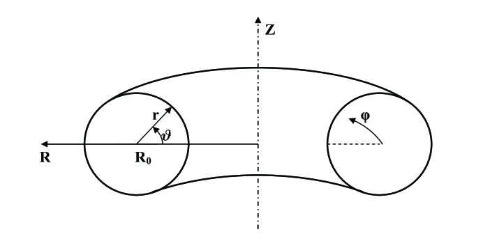
Figure 1: Axisymmetric toroidal solenoid

The force in the direction of the minor radius has two contributions:

$$F_{r}=j_{\vartheta}\,B_{\varphi}-j_{\varphi}\,B_{\vartheta}$$ (15)

Firstly, we consider a magnetic field which points only in toroidal direction and vanishes at the boundary $r=r_{b}$:

$$B_{\varphi}=C\frac{r_{b}^{2}-r^{2}}{2\,R}\;,\quad R=R_{0}-r\cos\vartheta$$ (16)

Insertion into the static equation (4) gives the current density components:

$$j_{\vartheta}=\frac{C}{\mu_{0}}\frac{r}{R}\;,\quad j_{r}=0$$ (17)

so that the magnetic force has the components:

$$F_{r}=\frac{C^{2}}{\mu_{0}}\frac{r\left({r_{b}^{2}-r^{2}}\right)}{2\,R^{2}}\;,\quad F_{\vartheta}=0$$ (18)

Now we must take the divergence of this force to obtain the Laplacian of the scalar potential:

$$\Delta p=\frac{C^{2}}{\mu_{0}\,R\,r}\frac{\partial}{\partial r}\left({\frac{R\,r^{2}\left({r_{b}^{2}-r^{2}}\right)}{2\,R^{2}}}\right)$$ (19)

Substitution into (11) yields the potential:

$$p\left({R,\,Z}\right)=\frac{-C^{2}}{4\pi\,\mu_{0}}\int\limits_{0}^{2\pi}{\int\limits_{0}^{2\pi}{\int\limits_{0}^{r_{b}}{\frac{1}{R^{\prime}\,r}\frac{\partial}{\partial r}\left({\frac{R^{\prime}\,r^{2}\left({r_{b}^{2}-r^{2}}\right)}{2\,R^{\prime 2}}}\right)}}}\frac{R^{\prime}\,r\,dr\,d\vartheta\,d\varphi}{\left|{\vec{x}-\vec{x}^{\prime}}\right|}$$

$$\left|{\vec{x}-\vec{x}^{\prime}}\right|=\sqrt{R^{2}+R^{\prime 2}-2\,R\,R^{\prime}\cos\varphi+\left({Z-r\sin\vartheta}\right)^{2}}\;,\quad R^{\prime}=R_{0}-r\cos\vartheta$$ (20)

Taking the rotation of (18) one obtains with (13) for the toroidal component of the vector potential:

$$u_{\varphi}\left({R,\,Z}\right)=\frac{-C^{2}}{4\pi\,\mu_{0}}\int\limits_{0}^{2\pi}{\int\limits_{0}^{2\pi}{\int\limits_{0}^{r_{b}}{\frac{1}{r}\frac{\partial}{\partial\vartheta}\left({\frac{\,r\left({r_{b}^{2}-r^{2}}\right)}{2\,R^{\prime 2}}}\right)}}}\frac{\cos\varphi\,\,R^{\prime}\,r\,dr\,d\vartheta\,d\varphi}{\left|{\vec{x}-\vec{x}^{\prime}}\right|}$$ (21)

Rather than trying to evaluate these integrals analytically, we have calculated them numerically and compared the result for the force component in the midplane $Z=0$

$$F_{R}=\frac{\partial p}{\partial R}-\frac{\partial u_{\varphi}}{\partial Z}$$ (22)

with the analytic expression resulting from (18):

$$F_{R}=\frac{C^{2}}{\mu_{0}}\frac{\left({R-R_{0}}\right)\left({r_{b}^{2}-\left({R-R_{0}}\right)^{2}}\right)}{2\,R^{2}}$$ (23)

In Figure 2 the individual components of (22) are depicted together with their superposition and the analytic expression (23). The agreement between the numerical integrals (22) and the exact expression (23) is perfect within numerical accuracy. It is also observed that the individual contributions in (22) are finite outside the torus (which extends from $R=.5\;\mbox{to}\;\mbox{1.5})$, but cancel perfectly when they are superimposed. This result confirms the validity of Helmholtz’s theorem for the chosen case.

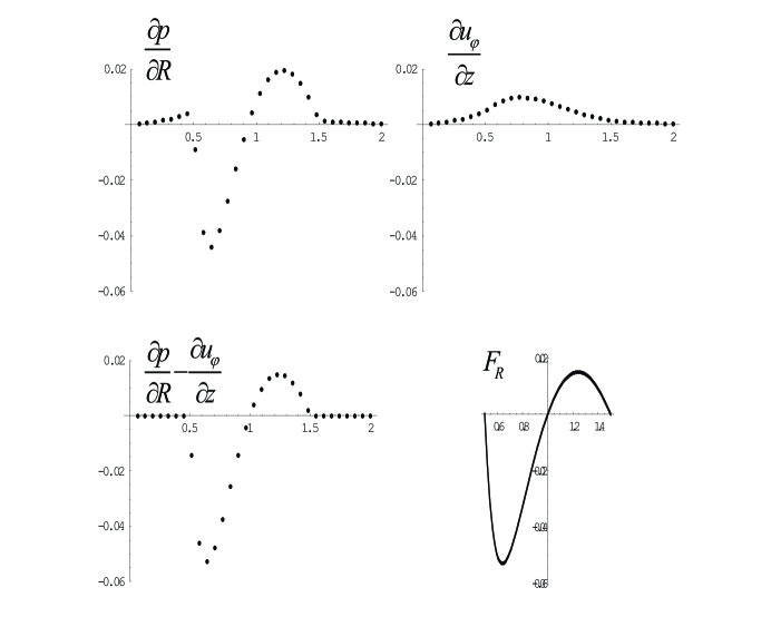
Figure 2: Radial magnetic force $F_{R}=j_{\vartheta}\,B_{\varphi}$ represented by potentials

Next we consider the second term in (15) which we choose finite on the torus surface. Assuming a magnetic field of the form

$$B_{\vartheta}=\frac{C\,r}{R}\;,\quad B_{r}=0$$ (24)

we obtain with (4) the toroidal component of the current density:

$$j_{\varphi}=\frac{C\left({R_{0}+R}\right)}{\mu_{0}\,R^{2}}$$ (25)

and with (15) the magnetic force component:

$$F_{r}=-\frac{C^{2}\,r\,\left({R_{0}+R}\right)}{\mu_{0}\,R^{3}}$$ (26)

Taking divergence and rotation of this expression we obtain with (11) and (13) the integral representation of the potentials:

$$p\left({R,\,Z}\right)=\frac{C^{2}}{4\pi\,\mu_{0}}\int\limits_{0}^{2\pi}{\int\limits_{0}^{2\pi}{\int\limits_{0}^{r_{b}}{\frac{1}{R^{\prime}\,r}\frac{\partial}{\partial r}\left({\frac{R^{\prime}\,r^{2}\,\left({R_{0}+R^{\prime}}\right)}{R^{\prime 3}}}\right)}}}\frac{R^{\prime}\,r\,dr\,d\vartheta\,d\varphi}{\left|{\vec{x}-\vec{x}^{\prime}}\right|}$$ (27)

$$u_{\varphi}\left({R,\,Z}\right)=\frac{C^{2}}{4\pi\,\mu_{0}}\int\limits_{0}^{2\pi}{\int\limits_{0}^{2\pi}{\int\limits_{0}^{r_{b}}{\frac{1}{r}\frac{\partial}{\partial\vartheta}\left({\frac{\,r\,\left({R_{0}+R^{\prime}}\right)}{R^{\prime 3}}}\right)}}}\frac{\cos\varphi\,\,R^{\prime}\,r\,dr\,d\vartheta\,d\varphi}{\left|{\vec{x}-\vec{x}^{\prime}}\right|}$$ (28)

The radial force in the midplane may be derived from these integrals with (22) and compared with the analytic expression:

$$F_{R}=\frac{C^{2}\,\left({R^{2}-R_{0}^{2}}\right)}{\mu_{0}\,R^{3}}$$ (29)

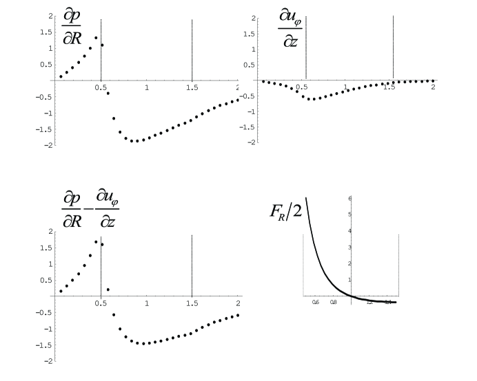
Figure 3: Radial magnetic force $F_{R}=-j_{\varphi}\,B_{\vartheta}$ represented by potentials

In Figure 3 we show the result. Obviously, the force as derived from the potentials (27) and (28) bears little resemblance with the given force $F_{R}$ (note that the scale of the $F_{R}$ - plot has been reduced by a factor of 2 in Fig. 3). Furthermore, the superposition of the derivatives of the potentials does by no means vanish outside the torus. As already mentioned, this behaviour is to be expected for integrals like (27) and (28), in particular, when the force is finite on the boundary as in (26). This holds also for the electric force – the first term in (1) – when the body carries a total charge resulting in a finite boundary field. Helmholtz’s theorem is apparently not applicable when the vector field is discontinuous which is a common property of the electromagnetic forces except in specially constructed cases like (16).

Our investigation so far reveals that the Helmholtz formalism for determining the potentials from which the electromagnetic forces could be derived will fail in most practical instances. On the other hand, physical differential equations like (8) or (9) can only have a solution, when the electric potential or the pressure do exist. It is therefore of great importance to explore different methods which seek a solution for the potentials. The next Section will deal with standard methods being used in plasma physics for obtaining solutions to the potential problem of the electromagnetic forces.

3 Standard methods for solving first order vector field equations in plasma physics

3.1 Ohm’s law in a plasma

In an early paper of 1958 Kruskal and Kulsrud [3] examined the conditions under which a plasma can be confined by a magnetic field. They realized that Ohm’s law (9) leads in conjunction with Faraday’s law and the assumption of a steady state to a special first order equation $-\vec{B}\cdot\nabla\Phi=\eta\,\vec{j}\cdot\vec{B}$, since the electric field should be expressible as the gradient of a scalar, if $rot\,\vec{E}=0$. For this type of equation they coined the term ‘magnetic differential equation’. Newcomb [4] formulated a solvability criterion $\oint{\left({{\eta\,\vec{j}\cdot\vec{B}}\mathord{\left/{\vphantom{{\eta\,\vec{j}\cdot\vec{B}}B}}\right.\kern-1.2pt}B}\right)}\,dl=0$, where the integration has to be carried out along closed magnetic field lines. Pfirsch and Schlüter [5] made an attempt to solve the magnetic differential equation without taking reference to Helmholtz’s theorem, although in effect they were trying to determine the gradient part of (9). They used a magnetic model field in the geometry of Figure 1 where the poloidal field lines closed themselves on circles. This field satisfied Maxwell’s equation (5), but not exactly (4) and the force equilibrium condition (8). Nevertheless, they obtained an estimate for the plasma diffusion coefficient in a toroidal configuration. Later on Maschke [6] generalized their results for a true equilibrium configuration that was supposed to satisfy both (4) and (8). He was able to confirm the order of magnitude of the predicted plasma losses. The present state of the art to calculate collisional transport in tokamaks including the effect of trapped particles can be found, e.g., in [7].

Following the method originally adopted in [6] we assume that an axisymmetric toroidal field configuration exists (e.g. ‘tokamak’ [8]), where the poloidal magnetic field components may be derived from the toroidal component of a vector potential:

$$B_{R}=-\frac{1}{R}\frac{\partial\psi}{\partial Z}\;,\quad B_{Z}=\frac{1}{R}\frac{\partial\psi}{\partial R}\;,\quad\psi=R\,A_{\varphi}$$ (30)

The poloidal field lines follow the contours of the surfaces $\psi=\mbox{const}$ which are nested, but not necessarily concentric circles as in Figure 1. The inner product of (9) with the magnetic field yields the magnetic differential equation:

$$B_{R}\,E_{R}+B_{Z}\,E_{Z}=\eta\,\vec{j}\cdot\vec{B}-E_{\varphi}\,B_{\varphi}=s$$ (31)

In steady state the poloidal electric field components may be expressed as the gradient of a potential, whereas the toroidal component $E_{\varphi}=U\mathord{\left/{\vphantom{UR}}\right.\kern-1.2pt}R$ could be induced by a transformer that produces a loop voltage $U$. The authors of [3, 4, 5, 6] assumed that (31) has a solution which means that a potential exists such that one can write:

$$B_{R}\,\frac{\partial\phi}{\partial R}+B_{Z}\,\frac{\partial\phi}{\partial Z}=-s$$ (32)

This equation specifies the derivative of the potential along the poloidal field lines. Straightforward integration over the contours of constant flux yields the ‘potential’

$$\phi=\phi_{0}\left(\psi\right)-\int\limits_{l_{0}}^{l}{\frac{R\,s}{\left|{\nabla\psi}\right|}}\,dl$$ (33)

where $dl$ is a line element on a contour $\psi=\mbox{const}$. Newcomb’s criterion imposes the integrability condition

$$\oint\limits_{\psi=\mbox{const}}{\frac{R\,s}{\left|{\nabla\psi}\right|}}\,dl\,=0$$ (34)

which must be satisfied by $s$ in order to avoid a multi-valued potential.

Although the described procedure yields a function $\phi\left({\psi,\,l}\right)$ in a ‘flux coordinate system’, one cannot be certain whether it represents a potential which exists independently of the chosen coordinate system. This would be guaranteed if we had obtained the potential from the solution of a Poisson equation like (11), but this was not possible, as we do not have – at this point – any information on the velocity field that determines the Laplacian of the potential according to (9):

$$\Delta\phi=\vec{B}\cdot rot\,\vec{v}-\vec{v}\cdot rot\,\vec{B}$$ (35)

There is only some knowledge on the current and field configuration which enters into $s$ as defined by (31). Maybe this was the reason why the Helmholtz method was ignored in the analysis of plasma equilibria.

In order to guarantee the existence of the potential in any coordinate system, we must satisfy the necessary and sufficient condition $rot\,\vec{E}=0$, or:

$$\frac{\partial E_{R}}{\partial Z}=\frac{\partial E_{Z}}{\partial R}$$ (36)

We can apply this condition when we take the gradient of (31)

$$B_{R}\frac{\partial E_{R}}{\partial R}+B_{Z}\frac{\partial E_{Z}}{\partial R}+E_{R}\frac{\partial B_{R}}{\partial R}+E_{Z}\frac{\partial B_{Z}}{\partial R}=\frac{\partial s}{\partial R}$$

(37)

$$B_{R}\frac{\partial E_{R}}{\partial Z}+B_{Z}\frac{\partial E_{Z}}{\partial Z}+E_{R}\frac{\partial B_{R}}{\partial Z}+E_{Z}\frac{\partial B_{Z}}{\partial Z}=\frac{\partial s}{\partial Z}$$

and derive with (36) and (5) two magnetic differential equations for the electric field components:

$$\vec{B}\cdot\nabla\left({\frac{E_{R}}{R\,B_{Z}}}\right)=\frac{1}{R}\frac{\partial}{\partial R}\left({\frac{s}{B_{Z}}}\right)\;,\quad\vec{B}\cdot\nabla\left({\frac{E_{Z}}{R\,B_{R}}}\right)=\frac{1}{R}\frac{\partial}{\partial Z}\left({\frac{s}{B_{R}}}\right)$$ (38)

The solutions are in analogy to (33):

$$E_{R}=R\,B_{Z}\left[{f_{R}\left(\psi\right)+I_{R}\left({\psi,\,l}\right)}\right]\;,\quad I_{R}\left({\psi,\,l}\right)=\int\limits_{l_{0}}^{l}{\frac{\partial}{\partial R}\left({\frac{s}{B_{Z}}}\right)}\frac{dl}{\left|{\nabla\psi}\right|}$$

$$E_{Z}=R\,B_{R}\left[{f_{Z}\left(\psi\right)+I_{Z}\left({\psi,\,l}\right)}\right]\;,\quad I_{Z}\left({\psi,\,l}\right)=\int\limits_{l_{0}}^{l}{\frac{\partial}{\partial Z}\left({\frac{s}{B_{R}}}\right)}\frac{dl}{\left|{\nabla\psi}\right|}$$ (39)

where Newcomb’s condition (34) must also be satisfied.

Instead of cylindrical coordinates one could also have used spherical coordinates with $R=r\,\sin\theta\,,\;Z=r\,\cos\theta\,,\;B_{R}=B_{r}\,\sin\theta+B_{\theta}\,\cos\theta,\;B_{Z}=\,B_{r}\,\cos\theta-B_{\theta}\sin\theta\,$. Equation (31) transforms then into:

$$B_{r}\,E_{r}+B_{\theta}\,E_{\theta}=s$$ (40)

and the steady state condition $rot\,\vec{E}=0$ becomes:

$$\frac{\partial E_{r}}{\partial\theta}=\frac{\partial\left({r\,E_{\theta}}\right)}{\partial r}$$ (41)

Taking now the gradient of (40) one obtains with (5) and (41) the magnetic differential equations for the field components in the form:

$$\vec{B}\cdot\nabla\left({\frac{E_{r}}{R\,B_{\theta}}}\right)=\frac{1}{R\,r}\frac{\partial}{\partial r}\left({\frac{r\,s}{B_{\theta}}}\right)\;,\quad\vec{B}\cdot\nabla\left({\frac{E_{\theta}}{R\,B_{r}}}\right)=\frac{1}{R\,r}\frac{\partial}{\partial\theta}\left({\frac{s}{B_{r}}}\right)$$ (42)

with the solutions:

$$E_{r}=R\,B_{\theta}\left[{f_{r}\left(\psi\right)+I_{r}\left({\psi,\,l}\right)}\right]\;,\quad I_{r}\left({\psi,\,l}\right)=\int\limits_{l_{0}}^{l}{\frac{1}{r}\frac{\partial}{\partial r}\left({\frac{s\,r}{B_{\theta}}}\right)}\frac{dl}{\left|{\nabla\psi}\right|}$$

$$E_{\theta}=R\,B_{r}\left[{f_{\theta}\left(\psi\right)+I_{\theta}\left({\psi,\,l}\right)}\right]\;,\quad I_{\theta}\left({\psi,\,l}\right)=\int\limits_{l_{0}}^{l}{\frac{1}{r}\frac{\partial}{\partial\theta}\left({\frac{s}{B_{r}}}\right)}\frac{dl}{\left|{\nabla\psi}\right|}$$ (43)

The same expressions must result, if we transform the solutions (S0.Ex4) directly into spherical coordinates:

$$E_{r}\,\sin\theta+E_{\theta}\,\cos\theta=R\,\left({B_{r}\,\cos\theta-B_{\theta}\sin\theta\,}\right)\left[{f_{R}\left(\psi\right)+I_{R}\left({\psi,\,l}\right)}\right]\;$$

(44)

$$E_{r}\,\cos\theta-E_{\theta}\sin\theta\,=R\,\left({B_{r}\,\sin\theta+B_{\theta}\,\cos\theta}\right)\left[{f_{Z}\left(\psi\right)+I_{Z}\left({\psi,\,l}\right)}\right]\;$$

or:

$$\!\!\!E_{r}\!=\!R\,B_{r}\sin\theta\cos\theta\left[{f_{R}+I_{R}+f_{Z}+I_{Z}}\right]+R\,B_{\theta}\!\left[{\cos^{2}\theta\left({f_{Z}+I_{Z}}\right)-\sin^{2}\theta\left({f_{R}+I_{R}}\right)}\right]$$

(45)

$$\!\!\!E_{\theta}\!=\!R\,B_{r}\!\left[{\cos^{2}\theta\left({f_{R}+I_{R}}\right)-\sin^{2}\theta\left({f_{Z}+I_{Z}}\right)}\right]-R\,B_{\theta}\sin\theta\cos\theta\left[{f_{R}+I_{R}+f_{Z}+I_{Z}}\right]$$

In order to make (S0.Ex8) compatible with (S0.Ex5) it is apparently necessary to require:

$$f_{R}+I_{R}+f_{Z}+I_{Z}=0$$ (46)

On the other hand, if one substitutes the solution (S0.Ex4) into (31), one obtains:

$$R\,B_{R}\,B_{Z}\left({f_{R}+I_{R}+f_{Z}+I_{Z}}\right)=s$$ (47)

The inhomogeneous part $s$ of the magnetic differential equation (32) must apparently vanish, if the function $\phi$ is to exist as a potential independent of the coordinate system. This means, of course, that a scalar potential for the arbitrarily given vector field $\eta\,\vec{j}-\vec{v}\times\vec{B}$ in (9) does not exist. Only a function $\phi=\phi_{0}\left(\psi\right)$ would satisfy Ohm’s law (32) when $s=0$, but one could not consider it as a true potential either. This will be discussed in the following subsection.

3.2 The force equilibrium in a plasma

The stationary force balance in a magnetized plasma cannot be easily satisfied. In fact, there are not any analytic solutions of (8) known, except in the axisymmetric case [9, 10]. From the toroidal component of (8), namely $j_{Z}B_{R}-j_{R}B_{Z}=0$, follows with (4) a homogeneous magnetic differential equation for the toroidal field component:

$$\vec{B}\cdot\nabla\left({R\,B_{\varphi}}\right)=0$$ (48)

and the inner product of (8) with the magnetic field leads to another homogeneous magnetic differential equation

$$\vec{B}\cdot\nabla p=0$$ (49)

Inserting the obvious solutions:

$$B_{\varphi}={F\left(\psi\right)}\mathord{\left/{\vphantom{{F\left(\psi\right)}{R\;,\quad}}}\right.\kern-1.2pt}{R\;,\quad}p=p\left(\psi\right)$$ (50)

into the poloidal components of (8) one finds with (4) an expression for the toroidal component of the current density:

$$j_{\varphi}=R\frac{dp}{d\psi}+\frac{F}{\mu_{0}\,R}\frac{dF}{d\psi}$$ (51)

Substitution into the toroidal component of (4) yields with (30) the famous nonlinear Lüst-Schlüter-Grad-Rubin-Shafranov equation [11]:

$$\frac{\partial^{2}\psi}{\partial R^{2}}-\frac{1}{R}\frac{\partial\psi}{\partial R}+\frac{\partial^{2}\psi}{\partial Z^{2}}\equiv\Delta^{\ast}\psi=-\mu_{0}\,R^{2}\frac{dp}{d\psi}-F\,\frac{dF}{d\psi}$$ (52)

It is the basis for calculating numerically axisymmetric plasma equilibria. Recently the equation has been modified [12] to include approximately the effect of magnetic islands which break axisymmetry.

One must expect, however, that a function $p\left(\psi\right)$ which depends on a single vector component, namely $R\,\vec{e}_{R}\times A_{\varphi}\,\vec{e}_{\varphi}$, cannot represent a physical pressure that must be defined independent of the coordinate system. In order to see this we consider an analytical ‘Soloviev solution’ [9]

$$\psi=\frac{1}{2}\left({c_{0}R^{2}+b\,R_{0}^{2}}\right)Z^{2}+\frac{a-c_{0}}{8}\left({R^{2}-R_{0}^{2}}\right)^{2}\;,\quad F=\sqrt{F_{0}^{2}-2\,b\,R_{0}^{2}\,\psi}$$ (53)

which satisfies (52) by construction. The pressure is given as a linear function of $\psi$:

$$p\left({R,\,Z}\right)=p_{0}-\left({a\mathord{\left/{\vphantom{a{\mu_{0}}}}\right.\kern-1.2pt}{\mu_{0}}}\right)\,\psi=p_{0}-\left({a\mathord{\left/{\vphantom{a{\mu_{0}}}}\right.\kern-1.2pt}{\mu_{0}}}\right)\,R\,A_{\varphi}\left({R,\,Z}\right)$$ (54)

Transforming this equation into a Cartesian coordinate system yields:

$$p\left({x,\,y,\,z}\right)=p_{0}-\left({a\mathord{\left/{\vphantom{a{\mu_{0}}}}\right.\kern-1.2pt}{\mu_{0}}}\right)\,\left({x\,A_{y}-y\,A_{x}}\right)$$ (55)

Rotation of the coordinate system around the $y$ - axis by an angle $\alpha$ according to the transformation rules

$$x=x^{\prime}\cos\alpha-z^{\prime}\sin\alpha\;,\quad z=x^{\prime}\sin\alpha+z^{\prime}\cos\alpha\;,\quad y=y^{\prime}\quad\quad$$

(56)

$$A_{x}=A_{x^{\prime}}\cos\alpha-A_{z^{\prime}}\sin\alpha\;,\quad A_{z}=A_{x^{\prime}}\sin\alpha+A_{z^{\prime}}\cos\alpha\;,\quad A_{y}=A_{y^{\prime}}$$

results in a pressure field

$$p\left({x^{\prime},\,y^{\prime},\,z^{\prime}}\right)=p_{0}-\left({a\mathord{\left/{\vphantom{a{\mu_{0}}}}\right.\kern-1.2pt}{\mu_{0}}}\right)\,\left[{\left({x^{\prime}\,A_{y^{\prime}}-y^{\prime}\,A_{z^{\prime}}}\right)\cos\alpha+\left({y^{\prime}\,A_{z^{\prime}}-z^{\prime}\,A_{y^{\prime}}}\right)\sin\alpha}\right]\,$$ (57)

which depends not only on the new coordinates, but also on the rotational angle $\alpha$. It is, therefore, not a scalar in the usual definition: $p^{\prime}\left({\vec{x}^{\prime}}\right)=p\left({\vec{x}}\right)\;\mbox{for}\;\vec{x}^{\prime}=\vec{x}$. Our conclusion is then that the magnetic force $\vec{j}\times\vec{B}$ does not have a scalar potential which could be identified with a physical pressure.

The so-called ‘force-free’ configuration

$$\vec{j}\times\vec{B}=\vec{0}$$ (58)

which plays a role in very diluted astrophysical plasmas, deserves special mentioning. Obviously, it makes little sense to replace the $\vec{0}$ - vector in (58) by a gradient and a curl. Whether a solution to (58) exists, must be examined in a different way. In the axisymmetric case we have from (52):

$$\Delta^{\ast}\psi=-F\,\frac{dF}{d\psi}\equiv-g\left(\psi\right)$$ (59)

Applying Stokes’s theorem on this equation by integrating the toroidal current density over the area enclosed by a magnetic surface one has:

$$\oint{\frac{\left|{\nabla\psi}\right|}{R}}\,dl=\mathop{{\int\!\!\!\!\!\int}\mkern-21.0mu\bigcirc}{g\left(\psi\right)}\frac{dR\,dZ}{R}$$ (60)

With the inverse function

$$\psi=\int{\frac{F}{g\left(F\right)}}\,dF\;,\quad\nabla\psi=\frac{F}{g}\,\nabla F$$ (61)

one obtains from (59):

$$\Delta^{\ast}F=-\frac{g^{2}}{F}-\frac{g}{F}\left|{\nabla F}\right|^{2}\frac{d}{dF}\left({\frac{F}{g}}\right)$$ (62)

Stokes’s theorem applied on this equation gives:

$$\oint{\frac{\left|{\nabla F}\right|}{R}}\,dl=\mathop{{\int\!\!\!\!\!\int}\mkern-21.0mu\bigcirc}{\left({\frac{g^{2}}{F}+\frac{g}{F}\left|{\nabla F}\right|^{2}\frac{d}{dF}\left({\frac{F}{g}}\right)}\right)}\frac{dR\,dZ}{R}$$ (63)

Substitution of (61) into (60) yields on the other hand:

$$\frac{F}{g}\oint{\frac{\left|{\nabla F}\right|}{R}}\,dl=\mathop{{\int\!\!\!\!\!\int}\mkern-21.0mu\bigcirc}g\frac{dR\,dZ}{R}$$ (64)

Elimination of the line integral over the poloidal current density on the left-hand-sides of (63) and (64), and using (61) again results in an integral equation

$$g\,\mathop{{\int\!\!\!\!\!\int}\mkern-21.0mu\bigcirc}g\frac{dR\,dZ}{R}=F\mathop{{\int\!\!\!\!\!\int}\mkern-21.0mu\bigcirc}{\left({\frac{g^{2}}{F}+\frac{1}{F^{3}}\left({g^{2}-F\frac{dg}{d\psi}}\right)\left|{\nabla\psi}\right|^{2}}\right)}\frac{dR\,dZ}{R}$$ (65)

which can only be satisfied for $g=F{dF}\mathord{\left/{\vphantom{{dF}{d\psi=0}}}\right.\kern-1.2pt}{d\psi=0}$. This may be demonstrated by choosing $g=\mbox{const}$ and performing a partial integration on (65):

$$g^{2}\!\!\!\!\!\oint\limits_{\psi=\mbox{const}}\!\!\!\!\!{\frac{Z\left(R,\,\psi\right)dR\,}{R}}\,=F\,\frac{g^{2}}{F}\!\!\!\!\!\oint\limits_{\psi=\mbox{const}}\!\!\!\!\!{\frac{Z\left(R,\,\psi\right)dR\,}{\,R}}+F\mathop{{\int\!\!\!\!\!\int}\mkern-21.0mu\bigcirc}{\left({\frac{g^{3}\,Z}{F^{3}}\frac{\partial\psi}{\partial Z}+\frac{g^{2}}{F^{3}}\left|{\nabla\psi}\right|^{2}}\right)}\frac{dR\,dZ}{R}$$ (66)

The first term on the right-hand-side cancels against the left-hand-side, whereas the second term cannot vanish on every surface except for $g=0$. This may be verified by adopting the force-free Soloviev solution (53) with $a=0$ and $g=-b\,R_{0}^{2}$. We must conclude then that equation (58) in conjunction with Ampere’s law (4) does not have a solution.

4 Discussion and conclusion

Our attempts to determine scalar and vector potentials for the electromagnetic forces were only partially successful. Thanks to Helmholtz’s theorem the task of formulating and calculating the potentials should be an easy exercise, but it was found that in most practical cases – where the forces are discontinuous across the boundary of the conductors – the theorem is not applicable.

On the other hand, the potentials must exist, if the electromagnetic forces are to be balanced against mechanical forces in a stationary state, in particular in fluid conductors like plasmas, for example. We have examined the usual method for finding the electrostatic potential in Ohm’s law and the pressure potential in the force balance of a plasma without having regard to Helmholtz’s theorem. Although it appears possible to find solutions in specially chosen coordinate systems, the functions from which the forces may be derived cannot be identified with physical potentials, as they are not invariant against arbitrary transformations of the coordinate system.

Our finding has important implications on the physics of magnetic plasma confinement. If it is not possible to find solutions for the steady state equations, a plasma can only be confined in a ‘quasistationary’ state at best. This means that the partial time derivatives neither in the law of induction, nor in the equations of motion can be neglected. The plasma may develop into a fluctuating turbulent state where strict axisymmetry does not prevail anymore. The observed ‘anomaly’ of plasma losses is probably due to this lack of a well balanced equilibrium in confining devices like tokamaks, stellarators, reversed field pinches etc. Harold Grad – one of the authors of equation (52) – came in his last paper [13] to a similar conclusion: “The discovered lack of pressure balance is not a special consequence of one idealized model but carries over broadly to a variety of physical refinements and generalizations. Indeed, the mathematical result has profound physical consequences which have gradually entered the field in the context of rational rotation number resonances and multiple helicities, island formation, and turbulence.”

References

- [1] J. D. Jackson, Classical Electrodynamics, Second Edition, (JohnWiley & Sons, Inc., New York, 1975) Sect. 12, p. 607, eq. 12.141
- [2] G. Arfken, Mathematical Methods for Physicists, Third Edition, (Academic Press, Inc., Orlando, 1985) Chapter 1.15
- [3] M. D. Kruskal, R. M. Kulsrud, The Physics of Fluids 1 (1958) 265
- [4] W. A. Newcomb, The Physics of Fluids 2 (1959) 362
- [5] D. Pfirsch, A. Schlüter, Max-Planck-Institut für Physik und Astrophysik, Report MPI/Pa/7/62 (1962) (unpublished)
- [6] E. K. Maschke, Plasma Physics 13 (1971) 905
- [7] D. A. Gates, H. E. Mynick, R. B. White, Physics of Plasmas, 11 (2004) L45
- [8] John Wesson, Tokamaks, (Clarendon Press, Oxford, 1987)
- [9] S. Soloviev, Sov. Phys. JETP 26 (1968) 400; Zh. Eksp. Teor. Fiz. 53 (1967) 626
- [10] C. V. Atanasiu, S. Günter, K. Lackner, I. G. Miron, Physics of Plasmas 11 (2004) 35
-
[11]
R. Lüst, A. Schlüter, Zeitschrift für Naturforschung
12 (1957) 850
V. D. Shafranov, Sov. Phys. JETP 6 (1958) 545; Zh.Eksp.Teor. Fiz. 33 (1957) 710
H. Grad, H. Rubin, Proc. 2nd U. N. Int. Conf. on the Peaceful Uses of Atomic Energy Geneva 1958, Vol. 31, 190, Columbia University Press, New York (1959) - [12] X. Liu, J.D. Callen, C. G. Hegna, Physics of Plasmas 11 (2004) 4824L
- [13] H. Grad, International Journal of Fusion Energy 3 (1985) 33