Interplay between coarsening and nucleation in an Ising model with dipolar interactions

Abstract

We study the dynamical behavior of a square lattice Ising model with exchange and dipolar interactions by means of Monte Carlo simulations. After a sudden quench to low temperatures we find that the system may undergo a coarsening process where stripe phases with different orientations compete or alternatively it can relax initially to a metastable nematic phase and then decay to the equilibrium stripe phase through nucleation. We measure the distribution of equilibration times for both processes and compute their relative probability of occurrence as a function of temperature and system size. This peculiar relaxation mechanism is due to the strong metastability of the nematic phase, which goes deep in the low temperature stripe phase. We also measure quasi-equilibrium autocorrelations in a wide range of temperatures. They show a distinct decay to a plateau that we identify as due to a finite fraction of frozen spins in the nematic phase. We find indications that the plateau is a finite size effect. Relaxation times as a function of temperature in the metastable region show super-Arrhenius behavior, suggesting a possible glassy behavior of the system at low temperatures.

I Introduction

It is well known that the usual long range order characteristic of a ferromagnetic phase dominated by exchange interactions can be destroyed by the presence of dipolar interactions inducing the formation of magnetic domains Hubert and Schafer (1998). In some cases, typically when perpendicular anisotropy is present, the dipolar interactions are antiferromagnetic in character and compete with the ferromagnetic exchange interactions  Politi (1998); Giuliani et al. (2006) giving rise to antiferromagnetic or stripe phases. These phases are common in ferromagnetic thin films with perpendicular anisotropy and have been the subject of intense experimental Allenspach et al. (1990); Vaterlaus et al. (2000); Wu et al. (2004); Won et al. (2005); Portmann et al. (2006), theoretical Yafet and Gyorgy (1988); Pescia and Pokrovsky (1990); Abanov et al. (1995) and numerical MacIsaac et al. (1995); Cannas et al. (2004, 2006); Rastelli et al. (2006); Pighin and Cannas (2007); Carubelli et al. (2008) work in the last 20 years. In the strong anisotropy limit an ultrathin film can be modeled by a system of magnetic dipoles on a square lattice in which the magnetic moments are oriented perpendicular to the plane of the lattice, with both nearest-neighbor ferromagnetic exchange interactions and long-range dipole-dipole interactions between moments. The thermodynamics of this system is ruled by the dimensionless Ising Hamiltonian:

$${\cal H}=-\delta\sum_{<i,j>}\sigma_{i}\sigma_{j}+\sum_{(i,j)}\frac{\sigma_{i}\sigma_{j}}{r^{3}_{ij}}$$ (1)

where $\delta$ stands for the ratio between the exchange $J_{0}>0$ and the dipolar $J_{d}>0$ interactions parameters, i.e., $\delta=J_{0}/J_{d}$. The first sum runs over all pairs of nearest neighbor spins and the second one over all distinct pairs of spins of the lattice; $r_{ij}$ is the distance, measured in crystal units, between sites $i$ and $j$. The energy is measured in units of $J_{d}$. The equilibrium phase diagram of this system has been extensibly studied MacIsaac et al. (1995); Cannas et al. (2004); Rastelli et al. (2006); Pighin and Cannas (2007), while several dynamical properties at low temperatures were studied in Sampaio et al. (1996); Toloza et al. (1998); Stariolo and Cannas (1999); Gleiser et al. (2003). The threshold for the appearance of the stripe phase in this model is $\delta_{c}=0.425$ MacIsaac et al. (1995); Pighin and Cannas (2007). For $\delta>\delta_{c}$ the system presents a sequence of striped ground states, characterized by a constant width $h$, whose value increases exponentially with $\delta$ MacIsaac et al. (1995); Giuliani et al. (2006).

In Cannas et al. (2004) it was shown that in the range $1\leq\delta\leq 3$ the system presents a first order phase transition between a low temperature stripe phase and a high temperature tetragonal phase with broken translational and rotational symmetry. In a subsequent work Cannas et al. (2006) it was shown that for a narrow window around $\delta=2$ the model shows an intermediate nematic phase, between the stripe and tetragonal ones, where the system has short range positional order but long range orientational order. The nematic phase exists between two critical temperatures $T_{1}<T<T_{2}$. For finite sizes these are actually pseudo critical temperatures $T_{1}(L)$ and $T_{2}(L)$, with finite energy barriers between phases. The extrapolation to the thermodynamic limit gives $T_{1}(\infty)\approx 0.772$ and $T_{2}(\infty)\approx 0.797$ Cannas et al. (2006). For $L\sim 50$ ($L=48-56$) we can estimate $T_{1}(L)$ and $T_{2}(L)$ as the average between the positions of the minimum of the cumulant and the maximum of the specific heat, so $T_{1}(50)\approx 0.78$ and $T_{2}(50)\approx 0.81$. For the range of system sizes considered ($L\sim 50$) the energy barriers between the nematic and the tetragonal phases are rather small, while the barriers between the stripe and the nematic phases are very large Cannas et al. (2006). Hence, under a cooling from high temperature no metastable tetragonal states are observed, but we see a strong metastability in the nematic phase. This can be observed in Fig.19 of Ref.Cannas et al. (2006). Although metastability strongly resembles a first order phase transition, we were not able to determine the nature of the stripe-nematic transition unambiguously: while the nematic order parameter presents a jump at $T_{1}$ and the free energy barriers seem to diverge in the thermodynamic limit, the internal energy is continuous at the transition and the peak in the specific heat tends to saturate Cannas et al. (2006). Further MC simulations showed that the nematic phase is present also for other values of $\delta\neq 2$ in different parts of the phase diagram, mainly around the phase borders between striped states of different widths Pighin and Cannas (2007).

Here we study the out of equilibrium dynamical properties of the two dimensional Ising model with exchange and dipolar interactions described by the Hamiltonian (1) with $\delta=2$. We performed quenches of the system from initial conditions at high temperatures directly to the stripe phase ($T_{f}\leq T_{1}$). Our main result is the identification of two kinds of processes: a slow coarsening towards a metastable nematic phase followed by nucleation of the stripe phase in a background of the metastable nematic and also direct coarsening of the stripe phase without an intermediate nucleation process (see Fig.1). In each realization the system chooses one of both paths to the final stripe phase with probabilities that depend on the final temperature of the quench. We computed these probabilities from Monte Carlo simulations and then using arguments from homogeneous nucleation theory, finite size scaling analysis and known growth laws for critical dynamics we were able to characterize completely both kinds of processes in the whole temperature range below the stripe-nematic transition.

We also made slow cooling experiments, similar to those already discussed in Cannas et al. (2006) and which show strong hysteretic behavior in the energy. We confirm that hysteresis is associated with a strong metastability of the nematic phase, while the tetragonal phase shows negligible metastability in the energy under cooling. Finally, (quasi-)equilibrium autocorrelation functions obtained for a whole range of temperatures between the tetragonal and the stripes phases show slow relaxation characterized by stretched exponential decay. In the stripe phase the relaxation times obtained from the autocorrelations exhibit a strong growth which can be well fitted by a Vogel-Fulcher-Tamman relation, similar to the behavior of fragile glass formers, with a relatively high ( $T_{0}\simeq 0.45$) divergence temperature.

In Section II we describe the quench experiments and the associated phenomenology. In Section III the slow cooling experiments and the behavior of the equilibrium correlations are discussed. In Section IV we present a discussion of results and brief conclusions.

II Relaxation after a quench from high temperature: interplay between coarsening and nucleation

We performed quenches from infinite temperature (completely random initial configuration) down to temperatures $T<T_{1}$. We also compared with the case where the initial configuration is taken from an equilibrated state at temperatures $T\sim 1$. The results were the same.

The typical relaxation behavior can be appreciated in Fig.1, where we plotted the time evolution of the instantaneous energy per spin $E(t)/N$ for two different realizations of the stochastic noise, together with typical spin configurations along the evolution. We see that the system can relax through two different types of mechanisms. In Fig.1a the system relaxes first into a metastable nematic state, where it stays during a long time $\tau$, after which suddenly relaxes to the equilibrium striped state. In other words, there is a two-step relaxation: first a coarsening process, where domains of the nematic phase compete (horizontal and vertical stripe orientations), followed by a nucleation of the stable phase (we will verify this quantitatively later). In Fig.1b the system form domains of both the stable (striped) and metastable (nematic) phases that compete and relax directly to the equilibrium state through a coarsening process. Both types of relaxation processes can happen with certain probability which depends on the temperature. To analyze quantitatively these processes we computed the equilibration time probability distribution.

Figure 1: Time evolution of the energy per spin in a single MC run ($\delta=2$, L=52 and $T=0.65$) for two different realizations of the stochastic noise. Some snapshots of the spin configurations at different times are shown below the figures. (a) Competition between nematic domains (coarsening), that leads to a metastable nematic state, followed by an activated relaxation to the striped state (equilibration through nucleation); (b) Competition between nematic and striped domains (coarsening) that leads directly to equilibration.

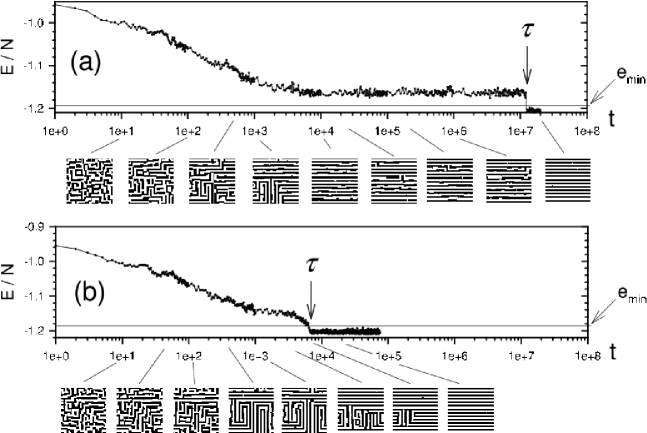
The equilibration time $\tau$ is defined as the time (in Monte Carlo Steps, MCS) that the system takes to reach the stable, crystal–like striped state after a quench. The criterium to determine $\tau$ was the following. For each quench temperature $T<T_{1}$ we calculated the equilibrium energy per spin histogram along a large single MC path starting from the ground state. This histogram presents two gaussian–shaped peaks, each one centered at the averages $u_{str}(T)$ and $u_{dis}(T)$ Cannas et al. (2006). Between the two peaks the histogram presents a finite minimum (at least for a finite system), associated with the free energy barrier that separates both phases. We also measured the standard deviation of the low energy peak associated with the striped phase $\sigma_{str}(T)$ and defined $e_{min}(T)=u_{str}+\sigma_{str}$, verifying that it is well below the central minimum of the histogram; $e_{min}$ is almost independent of the system size for $L\geq 32$, so it can be easily calculated using small system sizes. Then for each quench we calculated the average energy per spin $e(t)\equiv\left<H\right>/N$. When $e(t)$ fell bellow $e_{min}$ we stopped the simulation defining $e(\tau)=e_{min}$ (see Fig.1). Repeating this procedure we obtained the probability distribution (normalized frequency) $P(\tau)$ of the stochastic variable $\tau$ for different values of $T$ and $L$.

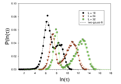
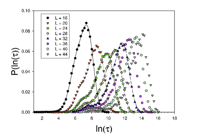
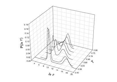
The above mentioned relaxation mechanisms are reflected in a characteristic two-peak structure in $P(\tau)$, each one centered at typical values corresponding to well different time scales, as shown in Figs.2 and 3. This probability distribution can be very well fitted using a superposition of two log–normal functions (see Figs.2 and 3) $P(\ln{\tau})=P_{1}(\ln{\tau})+P_{2}(\ln{\tau})$ with

$$P_{i}(\ln{\tau})=A_{i}\;\exp{\left(\frac{(\ln{\tau}-\mu_{i})^{2}}{2\;\sigma_{i}^{2}}\right)}\;\;\;\ i=1,2$$ (2)

where $A_{i}$ are normalization constants. Using these fittings we can see in Fig. 4 that the characteristic time scales of both peaks increases as $T$ decreases.

These fittings also allowed us to estimate the averages $\left<\tau\right>_{i}=\exp{\left(\mu_{i}+\sigma_{i}^{2}/2\right)}$, $i=1,2$, associated with each process. Both averages increase with $L$, so we can use finite size scaling analysis to determine the nature of the associated processes.

Figure 2: (Color online) Normalized frequency $P(\tau)$ vs $\ln{\tau}$ for $\delta=2$, $T=0.65$ and different system sizes. The lines correspond to a fitting with a superposition of two log-normal distributions. Sample size for the histograms were $\sim 2\times 10^{4}$.

Figure 3: (Color online) Normalized frequency $P(\tau)$ vs $\ln{\tau}$ for $\delta=2$, $T=0.77$ and different system sizes. The lines correspond to a fitting with a superposition of two log-normal distributions Eqs.(2). Sample sizes for the histograms run between $\sim 4\times 10^{3}$ ($L=44$) to $\sim 5\times 10^{4}$ ($L=16$).)

Figure 4: Fitted probability distribution $P(\tau)$ as a function of $\ln{\tau}$ and $T$ for $\delta=2$ and $L=24$.

II.1 Finite size scaling of the equilibration times

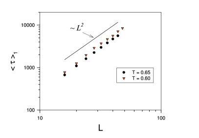
Suppose that the relaxation is completely governed by a competition between ground state domains, that is, by a curvature driven relaxation of the domain walls. The excess of energy respect to the ground state is given by $\delta e=\gamma n$, $\gamma$ being the "surface" tension per unit length of the domain walls and $n$ the fraction of spins belonging to them; $n$ is approximately given by $n\simeq bN_{d}(t)l(t)/N$, where $N_{d}(t)$ is the average number of domains, $l(t)$ is the average linear size of the domains and $b$ is a geometrical factor. Using $N_{d}\propto N/l^{2}(t)$ and grouping all these factors we get $\delta e\sim l^{-1}(t)$. For $\delta=2$ the energy distribution of the striped phase is very narrow and lies very near the ground state, so the criterium $e(\tau)=e_{min}$ implies $\delta e\ll 1$, condition that is attained when $l(\tau)\sim L$. Since for a heat bath dynamics with non-conserved order parameter (class A system) we can assume $l(t)\sim t^{1/2}$ we expect the scaling $\left<\tau\right>\sim L^{2}$. We verified that $\left<\tau\right>_{1}\sim L^{2}$ for a wide range of values of $T$ and $L$ (see an example in Fig.5), thus confirming that $P_{1}(\tau)$ is associated with a simple coarsening process.

Figure 5: (Color online) $\left<\tau\right>_{1}$ vs. L from two log-normal fittings Eqs.(2)

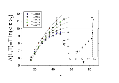
Now suppose that relaxation is governed by an homogeneous nucleation process. According to classical nucleation theory $\left<\tau\right>$ follows approximately an Arrhenius law $\left<\tau\right>=\tau_{0}\;\exp{(\Delta(L,T)/T)}$, $\Delta(L,T)$ being the height of the free energy barrier to nucleation. In a finite two–dimensional system Lee and Kosterlitz (1991) $\Delta(T_{m})\sim L$, $T_{m}$ being the melting temperature; in our case $T_{m}=T_{1}$. In an infinite system below the melting point, classical nucleation theory predicts that $\Delta(T)\equiv\Delta(\infty,T)$ is given by the excess of free energy of a critical droplet with average linear size $\xi(T)$ of the ordered (striped) phase inside the disordered (nematic) metastable state. Thus, if $L\gg\xi(T)$ the free energy barrier is expected to be almost independent of the system size when $T<T_{m}$. But, if $L<\xi(T)$, the droplet never reaches the critical size and the excess of free energy is dominated by surface tension. Hence, the transition to the crystal phase will occur when the crystal droplet reaches the system size and therefore we expect $\Delta(L,T)\sim L$ and $\ln{\left<\tau\right>}\sim L/T$. Fig.6 shows that $\left<\tau\right>_{2}$ follows such scaling, suggesting its identification with the average nucleation time $\tau_{nucl}$. However, due to the procedure we used to obtain it, $\left<\tau\right>_{2}$ actually corresponds to the crystallization time, which is not necessarily equal to $\tau_{nucl}$, because after the creation of a critical droplet it follows a growth process until the whole system reaches the crystal phase (for the rather small system sizes we considered we can assume that there is only one critical droplet). Hence, $\left<\tau\right>_{2}=\tau_{nucl}+\tau_{growth}$. However, we can expect $\tau_{growth}\sim L^{n}$, so $\tau_{nucl}\gg\tau_{growth}$, at least as far as $L$ is large enough that we are in the scaling regime, but small enough so that the free energy barrier still depends on $L$. Under these conditions $\left<\tau\right>_{2}$ give us a good approximation of $\tau_{nucl}$ and we can estimate $\Delta(L,T)\approx T\,\ln{\left<\tau\right>_{2}}$ up to logarithmic corrections. Then, by fitting the curves of Fig.6 using a sigmoidal function $\Delta(L,T)=\Delta(T)/\left(1+\exp{(L^{*}(T)-L)/c(T)}\right)$ ($L^{*}(T)$, $\Delta(T)$ and $c(T)$ are fitting parameters) we can extrapolate $\Delta(T)=\lim_{L\rightarrow\infty}\Delta(L,T)$. The extrapolated curve $\Delta(T)$ is shown in the inset of Fig.6. We see that $\Delta(T)$ grows strongly as $T\rightarrow T_{1}^{-}$, while it appears to present a minimum around $T=0.5$, or at least to saturate in a constant value as $T\rightarrow 0$. This is compatible with the results in Cannas et al. (2006) obtained from a different analysis where it was found a divergent free energy barrier at the transition temperature $T_{1}$ in the thermodynamic limit. For quench temperatures $T<0.5$ very large relaxation times make it very difficult to obtain reliable numerical results. For future analysis we list in Table 1 the approximated fitted values of $\left<\tau\right>_{2}$ for different values of $L$ and $T$.

Figure 6: (Color online) Estimated free energy barrier $\Delta(L,T)\approx T\,\ln{\left(\left<\tau\right>_{2}\right)}$ vs. $L$ for different temperatures. The dashed lines correspond to a sigmoidal fitting. The inset shows the extrapolated free energy barrier $\Delta(T)=\Delta(\infty,T)$ vs. $T$. The error bars are shown only when larger than the symbol size.

Figure 7: (Color online) Relative probability Eq.(3) vs. $T$ for $\delta=2$ and different values of $L$.

	$T=0.60$	$T=0.65$	$T=0.70$	$T=0.75$	$T=0.77$
$L=32$	$\sim 1.3\times 10^{6}$	$\sim 5.4\times 10^{5}$	$\sim 2.8\times 10^{5}$	$\sim 1.6\times 10^{5}$	$\sim 2.0\times 10^{5}$
$L=36$	$\sim 2.4\times 10^{6}$	$\sim 1.1\times 10^{6}$	$\sim 5.7\times 10^{5}$	$\sim 3.3\times 10^{5}$	$\sim 4.7\times 10^{5}$
$L=40$	$\sim 3.4\times 10^{6}$	$\sim 2.0\times 10^{6}$	$\sim 1.1\times 10^{6}$	$\sim 8.0\times 10^{5}$	$\sim 1.0\times 10^{6}$
$L=44$	$\sim 5.3\times 10^{6}$	$\sim 3.0\times 10^{6}$	$\sim 2.0\times 10^{6}$	$\sim 1.4\times 10^{6}$	$\sim 1.6\times 10^{6}$
$L=48$	$\sim 6.6\times 10^{6}$	$\sim 4.4\times 10^{6}$	$\sim 3.3\times 10^{6}$	$\sim 2.1\times 10^{6}$

Table 1: $\left<\tau\right>_{2}$ for different values of $L$ and $T$.

We also calculated the relative probability of occurrence of nucleation and coarsening processes

$$\phi(T)\equiv\frac{P_{nucl}}{P_{coars}}=\frac{\int_{-\infty}^{\infty}P_{2}(\ln{\tau})d(\ln{\tau})}{\int_{-\infty}^{\infty}P_{1}(\ln{\tau})d(\ln{\tau})}=\frac{\sigma_{2}\;A_{2}}{\sigma_{1}\;A_{1}}$$ (3)

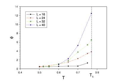
in the range $0.5\leq T<T_{1}$. In Fig.7 we see that $\phi(T)$ decreases monotonously with $T$. It seems to diverge as $T\rightarrow T_{1}^{-}$ and $L\rightarrow\infty$, while becoming almost independent of $L$ for $T<0.6$, saturating in a constant value $\phi\approx 0.5$. This shows that nucleation dominates the relaxation near the melting point, while coarsening becomes dominant for deep quenches, although there is always a finite and relatively high ($\sim 1/3$) probability of nucleation.

III Relaxation after a slow cooling

III.1 Energy

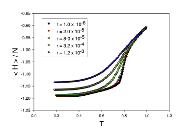
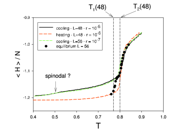
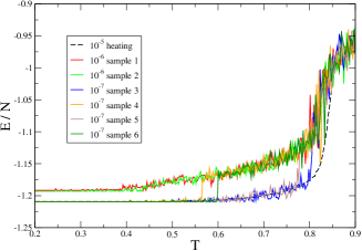
We first analyze the behavior of the average energy per spin during a slow cooling; that is, we first equilibrate the system at some temperature $T_{0}>T_{2}$ and then decrease the temperature down to a final value $T_{f}\ll T_{1}$ according to the linear protocol $T(t)=T_{0}-r\,t$, where $r$ is the cooling rate, $t$ is in MCS and the average is taken over several runs between $T_{0}$ and $T_{f}$. In Fig.8 we show an example. We see that below some value of $r$ the energy curve becomes almost independent of $r$. In Fig.9 we compare the cooling curves with the corresponding heating curve; this last curve is calculated by performing a linear heating from the ground state, starting at a very low temperature. We also compare the curves with the equilibrium values obtained in Ref.Cannas et al. (2006). These results verify that (for this range of system sizes) metastability in the tetragonal-nematic transition is negligible, while there is a strong metastability associated with the stripe-nematic transition. Notice that the metastable cooling curve has an inflection point around $T=0.5$ and falls down; although it does not reach the equilibrium value for $T<0.5$, this inflection point suggests the existence of a spinodal temperature around $T=0.5$. Moreover, from Table 1 we see that for $L\sim 50$ the nucleation time is $\tau_{nucl}\sim 4\times 10^{6}$ MCS; then, for a cooling rate $r=10^{-7}$, the time elapsed from the instant at which the temperature $T=T_{1}$ to the instant corresponding to a final temperature around $T=0.5$ will be $t=\Delta T/r\sim\tau_{nucl}$. Therefore, for that range of temperatures we would expect that in a large fraction of the realizations the system would have already equilibrated. Indeed, the results of Fig.10 verify this assumption. Moreover, the tracking of typical spin configurations for those realizations were the system did not equilibrate below $T=0.5$ shows that actually the system is no longer in a nematic state; instead of that, it got stuck in another metastable state, with a mixture of stripes with widths $h=2$ and $h=3$. Actually the $h=3$ striped phase becomes metastable precisely for that range of temperaturesPighin and Cannas (2007). This behavior reinforces the hypothesis of the existence of a spinodal temperature $T_{sp}\approx 0.5$. Also the behavior of the orientational order parameter observed in Fig.19 of Ref.Cannas et al. (2006) supports it.

Figure 8: (Color online) Average energy per spin in a cooling from $T=0.9$ ($\delta=2and$$L=48$) for different cooling rates.

Figure 9: (Color online) Average energy per spin cooling-heating curves ($\delta=2$ and $L=48$).

Figure 10: (Color online) Energy per spin cooling curves: individual realizations ($\delta=2$ and $L=48$).

III.2 Correlations

We now analyze the two-times correlation function

$$C(t_{w},t_{w}+t)=\frac{1}{N}\sum_{i}\left<S_{i}(t_{w})\;S_{i}(t_{w}+t)\right>$$ (4)

after a cooling from high temperature to a fixed temperature $T<T_{2}$. In this case we performed the cooling with a ladder protocol, that is, we reduced the temperature by steps of $\Delta T=0.01$, letting the system to equilibrate during $10^{4}$ MCS at each intermediate temperature. On the average, this corresponds to a cooling rate $r=10^{-6}$. Once we arrived to the measuring temperature (and after another $10^{4}$ MCS) we set $t=0$ and we saved the initial configuration. The autocorrelations (4) were then measured as a function of $t$ and $t_{w}$ and the whole curve was averaged over different realizations of the stochastic noise, starting always from the same initial configuration (this is to save CPU time). Some check repeating the calculation starting from different initial configurations (all obtained with the same cooling protocol) showed no difference with the previous one.

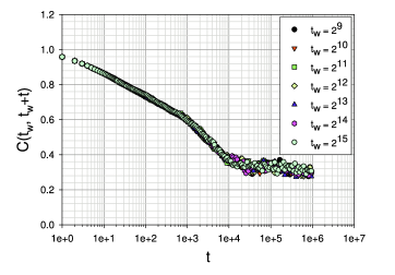
First of all we analyzed a cooling down to a temperature $T_{1}(L)<T<T_{2}(L)$, which corresponds to the stable region of the nematic phase. From Fig.11 we see that $C(t_{w},t_{w}+t)=C(t)$, as expected in a stable phase. We also noticed that the correlations do not decay to zero but to a plateau $C_{plateau}\approx 0.37$. We will discuss the meaning of that plateau later.

Figure 11: (Color online) Two-times correlation function $C(t_{w},t_{w}+t)$ as a function of $t$ for $\delta=2$, $L=48$ and different waiting times $t_{w}$, after a quasi-static cooling at $T=0.78$. Sample size for average was $150$

In Fig.12 we show the same calculation, but for a temperature $T<T_{1}(L)$. Both $t$ and $t_{w}$ were chosen such that $t+t_{w}\ll\tau_{nucl}$. We see that again $C(t_{w},t_{w}+t)=C(t)$, consistently with the expected quasi-stationary nature of a metastable state. We also see that the correlation also displays the characteristic plateau observed in the stable nematic state.

Figure 12: (Color online) Two-times correlation function $C(t_{w},t_{w}+t)$ as a function of $t$ for $\delta=2$, $L=48$ and different waiting times $t_{w}$, after a quasi-static cooling at $T=0.7$. Sample size for average was $350$

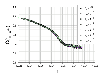
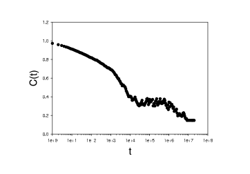
In Fig.13 we show $C(t)$ for $T=0.7$ and $L=48$ in a very long run with $t$ up to $2\times 10^{7}$ MCS. Comparing with table 1 we see that the second decay in the correlation coincides with the average nucleation time.

Figure 13: Correlation function $C(t)$ as a function of $t$ for $\delta=2$, $L=48$ and different waiting times $t_{w}$, after a quasi-static cooling at $T=0.7$. Sample size for average was $80$

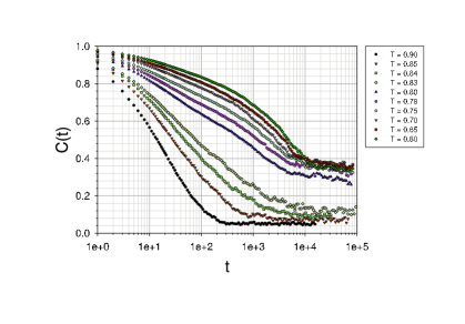
In Fig.14 we show $C(t)$ for $L=36$ and different cooling temperatures. We see that the plateau appears for any temperature, but becomes higher in the nematic case.

Figure 14: (Color online) Correlation function $C(t)$ as a function of $t$ for $\delta=2$ and $L=36$ after a quasi-static cooling at different final temperatures.

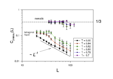
What is the origin of the plateau? In Fig.15 we show $C_{plateau}$ as a function of $L$ for different temperatures. For temperatures in the tetragonal liquid region, we see that for large enough sizes the plateau decays as $1/\sqrt{N}$, as expected in a disordered state. However, for small sizes the plateau is independent of $L$ and the crossover size increases as the temperature approaches $T_{2}$. Once we are in the nematic phase (either stable or metastable) the plateau for small sizes becomes independent of $T$ (at least for a range of temperatures where the relative probability of nucleation is high, see Fig. 7) and it is roughly equal to $1/3$. Since in a stationary state the unconnected correlations we are considering here behave as $C(t)\sim\frac{1}{N}\sum_{i}\left<S_{i}\right>^{2}$, this result shows that in the nematic state one third of the spins remain in a frozen state for small system sizes. Assuming then that the nematic state in a finite system is characterized by this residual correlation, we can define a normalized correlation function $C^{\prime}(t)$ as

Figure 15: (Color online) Correlation function plateau $C_{plateau}$ as a function of $L$ for $\delta=2$ and different temperatures.

$$C^{\prime}(t)\equiv\frac{\left(C(t)-C_{plateau}\right)}{\left(C(1)-C_{plateau}\right)}$$ (5)

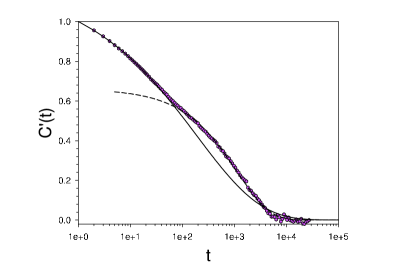
where $C^{\prime}(t)=0$ characterizes the equilibrium nematic state (either stable or metastable) . In Fig.16 we see the typical behavior of $C^{\prime}(t)$ for different temperatures from above $T_{2}$ down to temperatures well below $T_{1}$. Also $C^{\prime}(t)$ exhibit different behaviors above and below $T_{2}$. For temperatures above $T_{2}$ the curves are very well fitted (see Fig.16) by a modified stretched exponential function of the type

$$f(t)=A\;t^{\omega}e^{-\left(t/\tau\right)^{\gamma}}$$ (6)

Figure 16: (Color online) Normalized correlation function Eq.(5) as a function of $t$ for $\delta=2$ adn $L=36$, after a quasi-static cooling at different temperatures. The continuous lines for temperatures above $T_{2}$ correspond to fittings using Eq.(6).

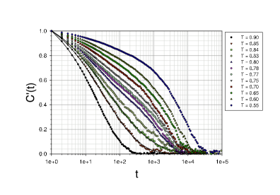
This fact is peculiar of the tetragonal liquid state: it does not exhibit exponential decay, even at relatively high temperatures. This behavior is observed also for $\delta=1$. For temperatures below $T_{1}$, $C^{\prime}(t)$ exhibit two different regimes, as can be appreciated more clearly in Fig.17. At short times $C^{\prime}(t)$ is again well fitted by a function of the type Eq.(6). For times longer that some crossover time, $C^{\prime}(t)$ enters into a pure stretched exponential regime, i.e., the best fit is obtained by a function of the type

$$f(t)=A\;e^{-\left(t/\tau\right)^{\gamma}}$$ (7)

Figure 17: Normalized correlation function Eq.(5) as a function of $t$ for $\delta=2$, after a quasi-static cooling at $T=0.78$. The continuous and dashed lines correspond to fittings using Eqs.(6) and (7) respectively.

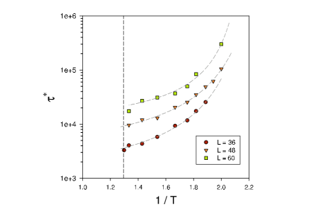
Finally, we analyzed the temperature dependence of the relaxation time $\tau$. Since there is too much uncertainty in fitting a curve with three parameters, instead of considering $\tau$ we defined another correlation time $\tau^{*}$ as the time at which $C^{\prime}(\tau^{*})=0.1$. In Fig.18 we see an Arrhenius plot of $\tau^{*}$ for different system sizes. The dashed lines in the figure correspond to fits using a Vogel-Fulcher-Tamman (VFT) form

$$\tau^{*}=\tau_{0}\exp{\left(\frac{A}{T-T_{0}}\right)}$$ (8)

which is usually associated with the behavior of relaxation times in a fragile glass-former, according to Angell’s classification Angell et al. (2000). The fitting values of $T_{0}$ for the different system sizes are shown in Table 2. We also show the fragility parameter $K\equiv T_{0}/A$, which show very high values around $K\approx 1$. It is worth mentioning that the data of Fig.18 can also be fitted with a power law of the type $\tau^{*}=A\,|T-T_{0}|^{-b}$. However, the best fitting is obtained with the VFT form Eq.(8).

$L$	$T_{0}$	K
$36$	$0.41\pm 0.025$	$1.20\pm 0.4$
$48$	$0.40\pm 0.015$	$1.25\pm 0.3$
$60$	$0.44\pm 0.075$	$2.10\pm 0.8$

Table 2: Fitting values of $T_{0}$ and the fragility parameter $K\equiv T_{0}/A$ for the relaxation time $\tau^{*}$ as a function of the supercooling temperature using a VFT form.

Figure 18: (Color online) Relaxation time $\tau^{*}$ vs. $1/T$ for $\delta=2$ and different system sizes. The dashed lines correspond to fittings using VFT form. The vertical line corresponds to $1/T_{1}$

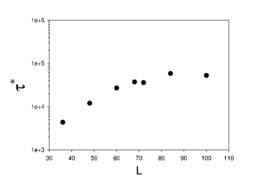
Notice the strong dependence of $\tau^{*}$ with $L$ for the range of sizes here considered. In Fig.19 we show $\tau^{*}$ as a function of $L$ for a fixed temperature in the metastable region. We see that $\tau^{*}$ becomes independent of $L$ for sizes larger than $L\sim 80$, which coincides with the crossover value observed for the plateau, suggesting the same origin for both finite size effects.

Figure 19: Relaxation time $\tau^{*}$ vs. $L$ for $\delta=2$ and $T=0.7$.

IV Discussion and conclusions

The main result of this work is the observation of interplay between nucleation and coarsening which appears to be a novel feature. In other words, coarsening happens usually as a competition between domains of different stable phases. In the present case both direct coarsening of the stripe phase and nucleation of the same phase on a nematic background can happen with a probability that depends on the final temperature. Nucleation processes are associated with a strong metastability of the nematic phase. If the final temperature $T_{f}<T_{1}$ is not too far below the stripe-nematic transition temperature the probability of nucleation is high: during the quench the system initially relaxes to the nematic phase, which is metastable below $T_{1}$ until finally it decays through nucleation to the equilibrium stripe phase. For final temperatures deep in the stripe phase simple coarsening processes between stripe states with different orientation have larger probability of occurrence than nucleation. Although no detailed theory is available for predicting this behavior in the whole temperature range, classical arguments assuming homogeneous nucleation, coarsening with a non-conserved order parameter and finite size scaling give a reasonably good interpretation of all the observed phenomenology. The origin of this interplay may rely in the fact that the stable and the metastable phases share the same orientational symmetry, so we can have domains with stripes (or pieces of stripes) that can be oriented along the same directions of the square lattice substrate in both phases.

Quasi-equilibrium autocorrelations in the stable and metastable nematic regions show a plateau whose nature is not completely clear. For temperatures where the nematic phase is only metastable, this plateau appears in a finite time window until a final decay for times $t\geq\tau_{nucl}$. For temperatures in the equilibrium nematic phase the behavior is more subtle. Although in a first approximation one could consider it to be a distinct characteristic of the nematic phase, in which a fraction of the spins remain practically frozen, we got indications that for the larger sizes the height of the plateau begins to diminish, signalling a possible finite size origin. One possibility is that the fraction of frozen spins in the nematic phase diminish with system size, in which case the plateau will eventually disappear for sizes large enough. More work is needed to clarify the behavior of equilibrium relaxations in large samples.

The present results also confirm the existence of the intermediate nematic phase, as observed in equilibrium simulations in Cannas et al. (2006); Pighin and Cannas (2007); all the dynamical observations are in agreement with the reported equilibrium results. In fact, a nematic phase with quasi-long-range order is expected to be generic in isotropic systems with competing interactions Barci and Stariolo (2007). Recent analytic results on a continous version of the present system show the presence of an isotropic-nematic transition which is in the Kosterlitz-Thouless universality class, while the stripe phase with true positional long range order turns out to be unstable for continous and isotropic systems in $d=2$ Barci and Stariolo (2007) in the thermodynamic limit, at variance with the discrete model studied here. Nevertheless, it is important to note that, although truly unstable in the thermodynamic limit, stripe domains grow already in the paramagnetic phase with decreasing temperature  Mulet and Stariolo (2007) and may be relevant for observations in finte size systems, like in simulations for example. In the present case, the stability of the low temperature stripe phase may be due to the symmetry breaking effect of the lattice and the sharp nature of the Ising domain walls. A unified interpretation of the nature of the transitions in the discrete and continous models is still lacking.

A final important point concerns the strong increase observed in the stationary relaxation time $\tau^{*}$ in the metastable nematic phase. Although a spinodal instability cannot be excluded, the stretched exponential relaxation and the super Arrhenius behavior of $\tau^{*}(T)$ point to an increasing cooperative and glassy behaviour of the dynamics. Indeed, a very similar behavior in a related model, namely the Coulomb frustrated model in 3d, has been interpreted as an evidence of fragile glass forming phenomenologyGrousson et al. (2002). Recent experimental results on Fe on Cu(100) ultrathin filmsPortmann et al. (2006) have suggested the possibility of a stripe-liquid to stripe-glass transition in the vicinity of the stripe ordering temperature. Stripe-glassy behaviour can be interpreted within the Frustration Limited Domain Theory Tarjus et al. (2005) or the Random First Order Transition  Schmalian and Wolynes (2000); Westfahl Jr et al. (2001) scenarios. We have not attempted a quantitative comparison with either theory, which remains as subject of future work.

V Acknowledgments

This work was partially supported by grants from CONICET, FONCyT grant PICT-2005 33305 , SeCyT-Universidad Nacional de Córdoba (Argentina), CNPq and CAPES (Brazil), and ICTP grant NET-61 (Italy).

References

- Hubert and Schafer (1998) A. Hubert and R. Schafer, Magnetic Domains (Springer-Verlag, Berlin, 1998).
- Politi (1998) P. Politi, Comments Cond. Matter Phys. 18, 191 (1998).
- Giuliani et al. (2006) A. Giuliani, J. L. Lebowitz, and E. H. Lieb, Physical Review B 74, 064420 (2006).
- Allenspach et al. (1990) R. Allenspach, M. Stamponi, and A. Bischof, Phys. Rev. Lett. 65, 3344 (1990).
- Vaterlaus et al. (2000) A. Vaterlaus, C. Stamm, U. Maier, M. G. Pini, P. Politi, and D. Pescia, Phys. Rev. Lett. 84, 2247 (2000).
- Wu et al. (2004) Y. Wu, C. Won, A. Scholl, A. Doran, H. Zhao, X. Jin, and Z. Qiu, Physical Review Letters 93, 117205 (2004).
- Won et al. (2005) C. Won, Y. Wu, J. Choi, W. Kim, A. Scholl, A. Doran, T. Owens, J. Wu, X. Jin, H. Zhao, et al., Phys. Rev. B 71, 224429 (2005).
- Portmann et al. (2006) O. Portmann, A. Vaterlaus, and D. Pescia, Phys. Rev. Lett. 96, 047212 (2006).
- Yafet and Gyorgy (1988) Y. Yafet and E. M. Gyorgy, Phys. Rev. B 38, 9145 (1988).
- Pescia and Pokrovsky (1990) D. Pescia and V. L. Pokrovsky, Phys. Rev. Lett. 65, 2599 (1990).
- Abanov et al. (1995) A. Abanov, V. Kalatsky, V. L. Pokrovsky, and W. M. Saslow, Phys. Rev. B 51, 1023 (1995).
- MacIsaac et al. (1995) A. B. MacIsaac, J. P. Whitehead, M. C. Robinson, and K. De’Bell, Phys. Rev. B 51, 16033 (1995).
- Cannas et al. (2004) S. A. Cannas, D. A. Stariolo, and F. A. Tamarit, Phys. Rev. B 69, 092409 (2004).
- Cannas et al. (2006) S. A. Cannas, M. Michelon, D. A. Stariolo, and F. A. Tamarit, Phys. Rev. B 73, 184425 (2006), URL http://link.aps.org/abstract/PRB/v73/e184425.
- Rastelli et al. (2006) E. Rastelli, S. Regina, and A. Tassi, Phys. Rev. B 73, 144418 (2006).
- Pighin and Cannas (2007) S. A. Pighin and S. A. Cannas, Physical Review B (Condensed Matter and Materials Physics) 75, 224433 (pages 9) (2007), URL http://link.aps.org/abstract/PRB/v75/e224433.
- Carubelli et al. (2008) M. Carubelli, O. V. Billoni, S. Pighin, S. A. Cannas, D. A. Stariolo, and F. A. Tamarit, Phys. Rev. B 77, 134417 (2008).
- Sampaio et al. (1996) L. C. Sampaio, M. P. de Albuquerque, and F. S. de Menezes, Phys. Rev. B 54, 6465 (1996).
- Toloza et al. (1998) J. H. Toloza, F. A. Tamarit, and S. A. Cannas, Phys. Rev. B 58, R8885 (1998).
- Stariolo and Cannas (1999) D. A. Stariolo and S. A. Cannas, Phys. Rev. B 60, 3013 (1999).
- Gleiser et al. (2003) P. M. Gleiser, F. A. Tamarit, S. A. Cannas, and M. A. Montemurro, Phys. Rev. B 68, 134401 (2003).
- Lee and Kosterlitz (1991) J. Lee and J. M. Kosterlitz, Phys. Rev. B 43, 3265 (1991).
- Angell et al. (2000) C. A. Angell, K. L. Ngai, G. B. M. Kenna, P. F. M. Millan, and S. W. Martin, Journal of Applied Physics 88, 3113 (2000).
- Barci and Stariolo (2007) D. G. Barci and D. A. Stariolo, Physical Review Letters 98, 200604 (pages 4) (2007), URL http://link.aps.org/abstract/PRL/v98/e200604.
- Mulet and Stariolo (2007) R. Mulet and D. A. Stariolo, Physical Review B (Condensed Matter and Materials Physics) 75, 064108 (pages 12) (2007), URL http://link.aps.org/abstract/PRB/v75/e064108.
- Grousson et al. (2002) M. Grousson, G. Tarjus, and P. Viot, Phys. Rev. E 65, 065103 (2002).
- Tarjus et al. (2005) G. Tarjus, S. A. Kivelson, Z. Nussinov, and P. Viot, Journal of Physics: Condensed Matter 17, R1143 (2005).
- Schmalian and Wolynes (2000) J. Schmalian and P. G. Wolynes, Phys. Rev. Lett. 85, 836 (2000).
- Westfahl Jr et al. (2001) H. Westfahl Jr, J. Schmalian, and P. G. Wolynes, Phys. Rev. B 64, 174203 (2001).