Vortex solitons in an off-resonant Raman medium
Abstract
We investigate existence and linear stability of coupled vortex solitons supported by cascaded four-wave mixing in a Raman active medium excited away from the resonance. We present a detailed analysis for the two- and three-component vortex solitons and demonstrate the formation of stable and unstable vortex solitons, and associated spatio-temporal helical beams, under the conditions of the simultaneous frequency and vortex comb generation.
I Introduction
Optical vortices are point phase singularities of the electromagnetic field, with the beam intensity vanishing at the singularity and the field phase changing by along any closed loop around it. is known as the orbital angular momentum quantum number or vortex charge. In a nonlinear medium vortices can propagate undistorted due to a balance between diffraction and nonlinearity, and form so-called vortex solitons Desyatnikov and Kivshar (2005). Nonlinearity can also trigger frequency conversion accompanied by the conversion of the charge . In particular, in the second harmonic generation process, the fundamental field carrying a vortex with the charge is converted into the second harmonic field with the charge Desyatnikov and Kivshar (2005); Buryak et al. (2002); Dholakia et al. (1996); Skryabin and Firth (1998); Torres et al. (1998a); Di Trapani et al. (2000). Analogous conversion rules have been reported for the degenerate four-wave mixing in Kerr-like materials Mihalache et al. (2003) and for the three-wave Raman resonant process Sogomonian et al. (2001). Multi-component vortex solitons sustained by the interaction of the beams with different frequencies in both quadratic and cubic materials are also well known, though under the most typical conditions the finite radius vortex solitons break into filaments due to azimuthal instabilities Desyatnikov and Kivshar (2005); Buryak et al. (2002); Skryabin and Firth (1998); Torres et al. (1998a).
While the above mentioned experimental and theoretical research of nonlinear vortex charge conversion has focused on cases involving a small number of frequency components, typically two or three, the efforts directed towards short pulse generation have resulted in the development of techniques leading to the generation of dozens of coherent frequency side-bands, by means of cascaded four-wave mixing in Raman active gases Sokolov and Harris (2003); Burzo et al. (2006). The latter technique does not rely on the waveguide or cavity geometries to boost nonlinear interaction and is therefore suitable for the simultaneous frequency and vortex charge conversion. This idea has been explored by our group and we have recently demonstrated simultaneous generation of frequency and vortex combs Gorbach and Skryabin (2007) in a Raman medium excited off-resonance with the two pump beams, when one of the two carries a unit vortex and the other is vortex free. We have derived the vortex conversion rules and demonstrated that the simultaneous frequency and vortex combs are shaped in the form of the spatio-temporal helical beams Gorbach and Skryabin (2007). On the focusing side of the Raman resonance, the multi-component vortex solitons have been found.
The aim of this work is to report regular tracing of the multi-component vortex solitons in the parameter space and to study their linear stability with respect to perturbations. Our analysis shows that the spectrally symmetric soliton solutions centered around the vortex-free frequency component are typically unstable, although the instability fully develops only after long propagation distances. At the same time, the asymmetric solitons, for example those where all the generated components are the Stokes ones, have a broad stability range. Based on the results of the linear stability analysis for 2 and 3 component solitons, we demonstrate the same general tendencies of the soliton dynamics for the case of many coupled side-bands.
II Model
The dimensionless model describing the evolution of the side-bands in an off-resonantly excited Raman medium is Sokolov and Harris (2003); Gorbach and Skryabin (2007)
| (1) |
where , and . are the dimensionless amplitudes of the sidebands, such that the total field is given by
| (2) |
where , is the modulation frequency (i.e. the frequency difference between the two driving fields). is the number of the anti-Stokes components and is the number of the Stokes components. Taking into account the field, we have interacting Raman side-bands. The physical frequencies and wavenumbers are represented by the lower case letters and , whilst their dimensionless counterparts by the upper case: and . The dimensionless time is measured in units of , the propagation coordinate is in units of , and the transverse coordinates are in units of . are the scaled free space wavenumbers. Here, characterizes the coupling length over which power is transferred between neighboring side-bands in the absence of dispersion. is the free space impedance, is the density of molecules and is a coefficient characterizing the material dependent coupling between the sidebands Sokolov and Harris (2003). The weak frequency dependence of is neglected for simplicity.
varies from to a few mm for and gases Sokolov and Harris (2003), so that one unit of corresponds to a few tens of microns. is the Raman coherence responsible for the coupling between the side-bands. Neglecting dissipation due to finite linewidth of atomic transition and finite dephasing time, in the adiabatic approximation Sokolov and Harris (2003); Gorbach and Skryabin (2007, 2006)
| (3) |
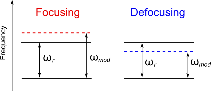
where is the scaled modulus of the detuning of the modulation frequency from the Raman frequency . We also note, that the above result is obtained under the assumption of equal Stark shifts of molecular levels, which is the case for large detunings Sokolov and Harris (2003). While can always be fixed to unity by proper rescaling of the field amplitudes, its sign controls the effective type of nonlinearity in Eqs. (1): positive (negative) corresponds to the focusing (defocusing) nonlinearity Gorbach and Skryabin (2007); Proite et al. (2008), see Fig. 1. In what follows we consider the case of the focusing nonlinearity Proite et al. (2008); Walker et al. (2002), (), which is known to support bright soliton solutions Yavuz et al. (2003); Yavuz (2007).
varies from to for varying from to . Therefore nonlinear interaction between harmonics is saturated at high powers or, equivalently, at small detunings . are the dimensional amplitudes of the harmonics. For and gases corresponds to GW/cm2, provided GHz. is the propagation constant of the th harmonic.
III Soliton solutions: General framework
In this and the next chapter we describe the general framework for finding the stationary soliton solutions and studying their linear stability. Application of these techniques to the cases of two and three components are described in detail in Chapters V and VI. The fact that equations (1), (3) are invariant with respect to and , where and are arbitrary constants Gorbach and Skryabin (2007, 2006), implies the conservation of the two integrals and , where , and suggests the following ansatz for the soliton solutions:
| (4) |
Here and are the polar radius and angle, is the vortex charge of the th harmonic, are free parameters associated with the above symmetries. The choice of and defines the step, , in which the vortex charge is changing between the adjacent side-bands. are real functions obeying
| (5) | |||||
where . The boundary conditions are Skryabin and Firth (1998):
| (6) | |||||
| (7) |
where are real constants. Eq. (6) naturally implies that the amplitude of a vortex carrying component, , is zero at the phase singularity and that the vortex free components, , reach some constant value at . For the fields to decay to zero at , one needs to select to satisfy
| (8) |
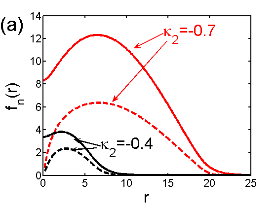
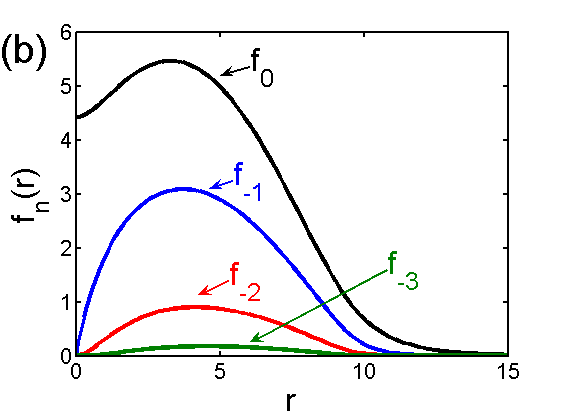
simultaneously for all . Without any loss of generality can always be set to zero by the rotation of the common phase Gorbach and Skryabin (2007). Thus, fixing we find that the above inequality for gives . At the boundary points of the above conditions tends to zero. Detuning the values away from these boundaries into the range where is increasing eventually leads to the coherence tending to its maximal value . Examples of the radial profiles of the vortex solitons are shown in Fig. 2 for the asymmetric configuration with only Stokes components being excited (). When the propagation constants are symmetric around the central component: , Eqs. (5) are invariant under the transformation , , . In this case solitons in the opposite configuration, with only anti-Stokes components being excited (), have exactly the same structure as those shown in Fig. 2.
In the vortex soliton case the limit is achieved not only through the growing amplitudes, but also through the expansion of the rings and flattening of their profiles. The soliton existence boundary corresponding to can be worked out neglecting the and dependence of . Subsequently one can disregard the left-hand sides in Eq. (5), assume and work out constraints on the and values from the solvability conditions of the resulting homogeneous equations: . Examples of the existence domains in the -plane can be seen in Figs. 3(a) and 7.
IV Linear stability analysis: General framework
Stability of the vortex solutions is of course an important problem, since similar solutions in other models are known to exhibit strong modulational instability along the rings Skryabin and Firth (1998); Torres et al. (1998a); miold . This instability can be suppressed by nonlocal nonlinearities Briedis et al. (2005); Skupin et al. (2007), and in some cases when the higher order nonlinearities (e.g. quintic) are assumed to dominate over the lower order ones (e.g. cubic), see, e.g., Mihalache et al. (2002, 2003). Our model is particularly interesting because, as we will demonstrate below, it allows the existence of a sufficiently broad parameter range, where stable vortex solitons exist with the local type of nonlinearity derived from the first principles. The latter is true since the nonlinearity in Eq. (1) is calculated from the Schrödinger equation for a Raman medium driven far from the resonance Sokolov and Harris (2003); Gorbach and Skryabin (2006).
In order to analyze the linear stability we add small perturbations to the vortex solitons and substitute the following ansatz
| (9) |
into Eqs. (1). After linearization we find:
| (10) |
where
| (11) | |||||
| (12) | |||||
| (13) | |||||
| (14) |
and .
Expanding perturbations into azimutal harmonics Skryabin and Firth (1998)
| (15) | |||||
we assume and derive the eigenvalue problem:
| (16) |
where . and are the matrix operators. Elements of are and they are defined in Eq. (12), and the elements of are
where is the Kronecker symbol. For a solution to be linearly unstable there must exist with . Boundary conditions for eigenstates are defined in a similar way to the boundary conditions for (see Eqs. (6)-(7)), but with being replaced by . We solve the eigenvalue problem in Eq. (16) numerically, replacing differential operators by the second-order finite differences. Note that accurate stability analysis of the multi-component solutions is rather complicated. Therefore we will reveal basic mechanisms of instabilities of coupled vortex solitons by focusing on two- and three-component configurations. Then we will demonstrate by numerical modeling of Eqs. (1), that the instability and stabilization mechanisms found in the simplest cases can be seen in the multi-component dynamics.
V Two-component vortex solitons
We start with the simplest configuration of two side-bands, that is () in Eqs. (1). This applies e.g. to the opposite circularly polarized driving fields and , when the cascaded generation of Stokes and anti-Stokes harmonics is forbidden due to angular momentum selection rules Yavuz et al. (2003). The propagation equations in this case are
| (18) | |||||
| (19) |
Eqs. (18, 19) explicitly express a known fact that the fields interacting via the Raman nonlinearity do not have nonlinear self-action. This property does not depend on the number of interacting components.
Bright (vortex free) spatial solitons in the two-component Raman model have been studied in Yavuz (2007); Yavuz et al. (2003) and the associated self-focusing effects have been observed in Proite et al. (2008); Walker et al. (2002). Also, there are closely related recent results on spatial solitons in Raman active liquids Fanjoux et al. (2006, 2008). The papers time have analyzed the two-component temporal Raman solitons existing in the presence of group velocity dispersion, i.e. when the transverse Laplacian is replaced with the 2nd-order time derivative. The above two-component model is also similar to that for the so-called holographic solitons Cohen et al. (2002).
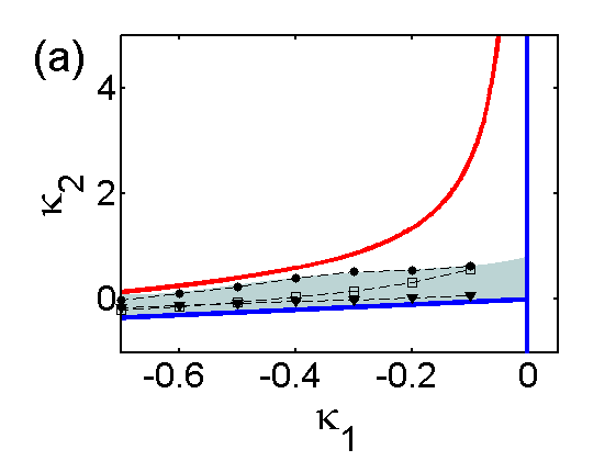
The existence conditions for soliton solutions in Eqs. (8) are reduced to the joint inequalities and , which define a semi-infinite region in bounded by the two rays, see Fig. 3(a). Another boundary is derived from the condition and is given by:
| (20) |
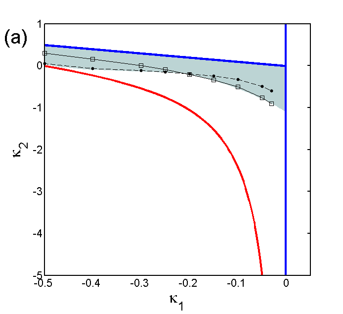
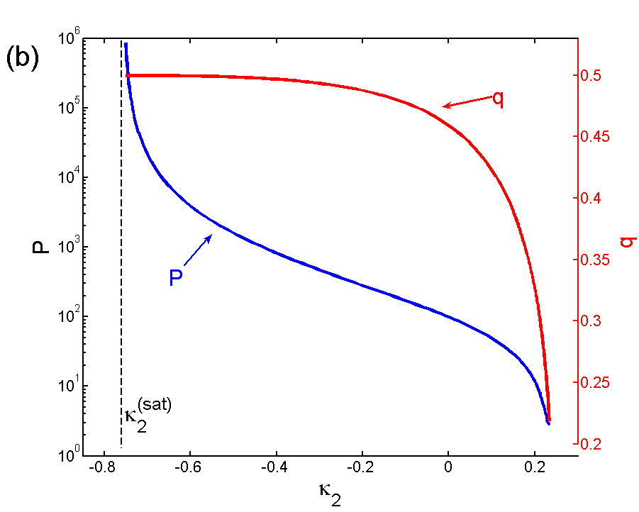
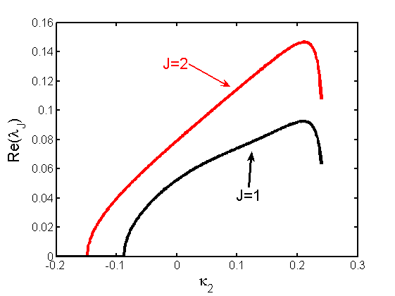
Our linear stability analysis demonstrates that the soliton with and is unstable only inside the sufficiently narrow range of corresponding to the relatively small values of , see Fig. 3. As soon as increases and the saturation effects become important the solution becomes stable. Note that the saturation of the self-focusing nonlinearity does not stabilize the vortices in the models with the nonlinear self-action effects Skryabin and Firth (1998). It suggests that the absence of the self-action plays an important role in stabilization of the vortex solitons. In its instability range, the vortex soliton is unstable with two eigenvalues and having positive real parts, see Fig. 4. Fixing we numerically find the critical values of , at which the two instabilities disappear, see circles and squares in Fig. 3(a). Selective numerical runs for the cases , and , suggest that they are unstable with respect to azimuthal instabilities through large parts of their existence domains.

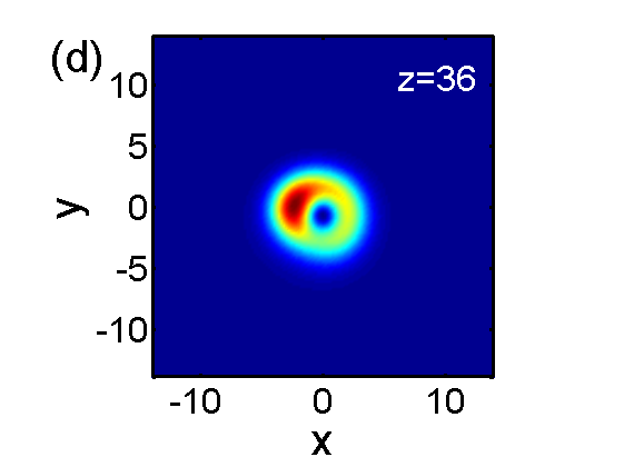
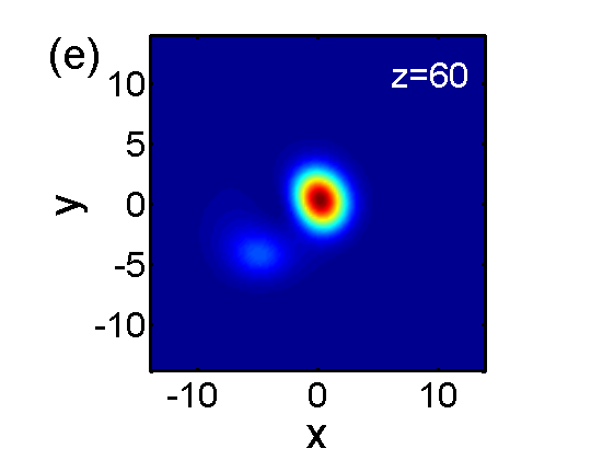
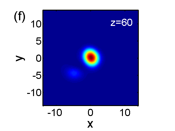
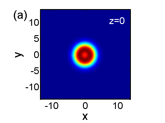
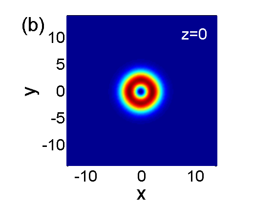
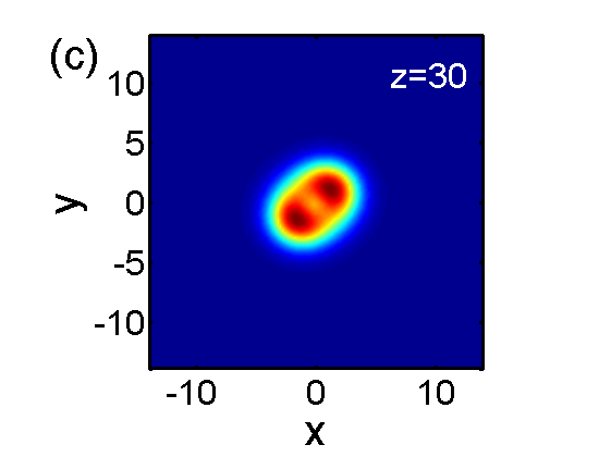
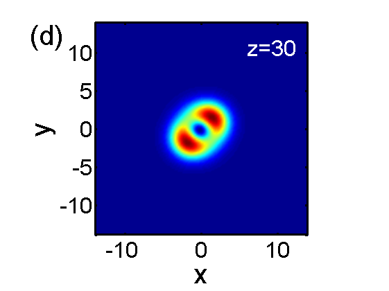
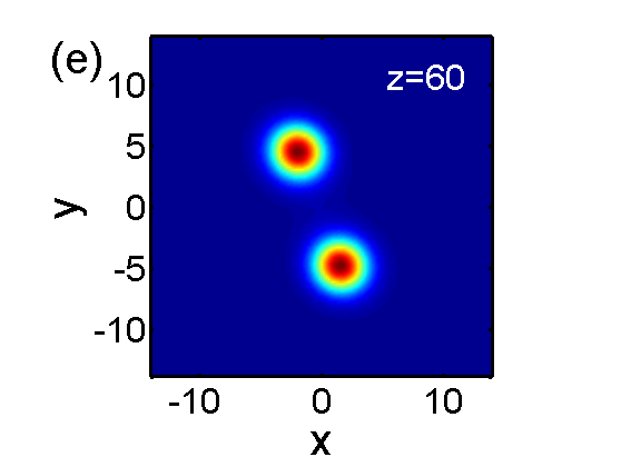
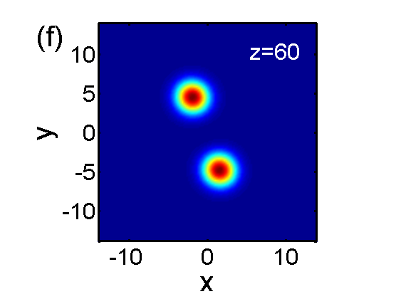
To reveal the impact of instabilities on the soliton dynamics, we initialize Eqs. (1) with numerically found soliton solutions slightly perturbed along unstable eigenvectors and perform dynamical simulations. Results are presented in Figs. 5 and 6 for the and unstable eigenvectors, respectively. Both perturbations break the soliton symmetry and eventually lead to the formation of a single or a pair of bright spatial solitons Yavuz et al. (2003); Yavuz (2007).
VI Three-component vortex solitons
The addition of the third component makes the interaction between the Raman side-bands phase-sensitive, and the choice of the vortex charges in any two fields defines the charge of the remaining field via the phase-matching conditions Gorbach and Skryabin (2007). Eqs. (1) for the three component case with are:
| (21) | |||
| (22) | |||
| (23) |
here . Fixing , we consider two cases ( and ): asymmetric and symmetric . The former corresponds to the often encountered case with negligible anti-Stokes side-bands, and the latter implies that the first Stokes and first anti-Stokes lines are excited.
The existence boundary for the asymmetric case given by the condition is now , where
| (24) |
In the symmetric case, the condition implies , where
| (25) |
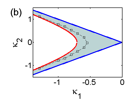
with . Together with the conditions in Eqs. (8), the above constraints define the regions of the soliton existence, see Fig. 7.
Stability analysis demonstrates that, similar to the two-component case with and , the three-component solitons with , , are stable inside a sufficiently wide domain in the plane and, in particular, in the proximity of the existence boundary given by , i.e. in the high saturation regime. Close to the lower boundary of the existence domain given by there are three types of instabilities with , see Fig. 7(a). We note that the solution with the side-bands generated on the anti-Stokes side, i.e. the solution with , , , has the same stability properties as the solution discussed above. The symmetric case with is found to be unstable with respect to the and instabilities, with the former one persisting in the entire existence domain, see Fig. 7(b).
VII Multi-component vortex solitons and spatio-temporal helical beams
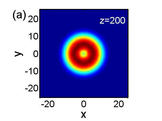
The above results show that if the vortex soliton contains a vortex free component, for example, at , and vortex carrying side-bands either only on the Stokes or only on the anti-Stokes sides, it can be stable within a broad range of parameters ensuring that the saturation effects are sufficiently strong. Since in the frequency comb generation experiments with the off-resonant Raman gases the total number of excited harmonics can go to a few dozen Sokolov and Harris (2003); Burzo et al. (2006), an important question to be addressed is whether the above stated principles of the vortex soliton stabilization can be extended onto multi-component cases. To address this problem we use numerical integration of Eqs. (1) with coupled side-bands, initialized with the three-component vortex solitons described in the previous section. We consider two cases: (i) asymmetric case where excitation of the anti-Stokes lines is suppressed, and (ii) symmetric case with excitation of Stokes and anti-Stokes lines being equally probable. In both cases we number the harmonics in a way that corresponds to the vortex-free component. Thus we take and in Eqs. (1) for the asymmetric and symmetric cases, respectively.
We monitor the evolution of the fields by plotting the total field intensity with defined in Eq. (2). It has been demonstrated in Gorbach and Skryabin (2007) that simultaneous frequency and vortex combs lead to the helical structure of the total field intensity , both in and subspaces. For the case of initial conditions where all the fields apart from the three pumps , and are initially zero, the can be crudely approximated with [see Appendix for details]:
| (26) |
where , is the vortex charge step between the neighboring side-bands and . For any fixed and the total intensity distribution in the transverse plane is modulated in with the period defined by , and it rotates in both and , forming a spatio-temporal helix.
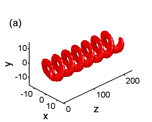
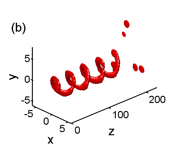
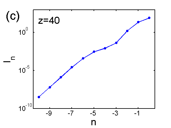
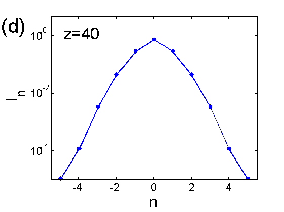

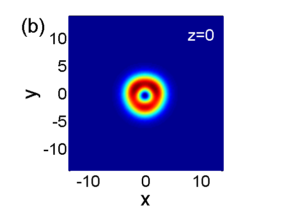
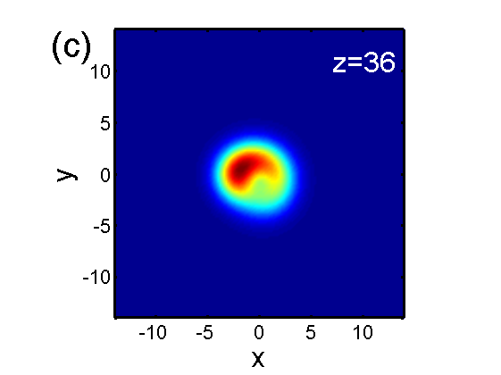
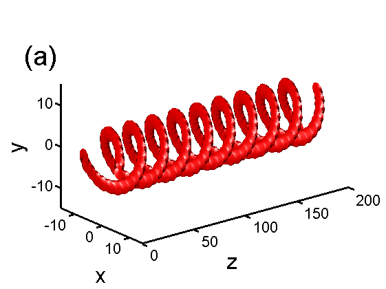
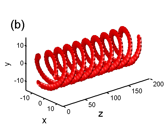
corresponds to the single-strand helical structure of , see Fig. 8 (a) and (b). Fig. 8 (a) shows the long distance evolution of the helix in the case of the asymmetric excitation, with all the side-bands generated on the Stokes side, see the corresponding spectrum in Fig. 8 (c). The resulting helix in this case keeps its structure fixed over considerable propagation lengths. A similar numerical experiment for the symmetric excitation results in the helical soliton, which breaks up into filaments after the same propagation distance, cf. Figs. 8(a) and (b). Note, however, that the total length in the simulations shown in Fig. 8 corresponds to a physical distance of order cm, which implies that one can speak about a quasi-stable propagation of the helix even in the case of the symmetric excitation of the Stokes and anti-Stokes side-bands. The -period of the helix, , is not a parameter of our numerical model, and it is only important when we are calculating . Physically realistic values of the adimensional period are of the order of (for a typical modulation frequency of the order of GHz Sokolov and Harris (2003)), which makes the helical structure contain several hundred periods over the distance of adimensional units required to see the instability. Therefore, to make the structure of the helices and the break-up process more obvious to the reader, we have fixed , when we have been producing the images of the helices in Figs. 8 and 10.
Providing the asymmetric excitation conditions and changing to 2 and 3, we have also observed the formation of the stable double- and triple-strand helices, see Fig. 10. Note that the formation of similar multiple-strand helices has been reported in Franke-Arnold et al. (2007), as a result of the linear superposition of the higher order Laguerre-Gauss modes. The helical soliton beams reported here are qualitatively different from the so-called spiraling solitons or rotating soliton clusters spir1 ; spir2 ; spir3 ; spir4 ; spir5 , which sustain their rotation due to the interaction between the individual beams accompanied by the conservation of the angular momentum. In our case the helical evolution does not require the presence of more than one intensity lobe, as shown in Fig. 8, and originates from the interaction of multiple frequency harmonics carrying progressively growing vortex charges. Most close known to us analogue of the spatio-temporal helices studied above have been reported in the context of the sine-Gordon equation and can be observed in a chain of coupled pendulums book .
VIII Summary
In this work we have reported existence conditions and have carried out linear stability analysis of the two and three component vortex solitons in an off-resonant Raman medium. We have found that, in the case where the vortex carrying Raman side bands are located either only on the Stokes or only on the anti-Stokes side of the vortex free component, the vortex solitons have a significant stability domain, corresponding to parameter values ensuring sufficient levels of nonlinearity saturation. We have also demonstrated that the same stabilization mechanisms work in the case of many side-band, leading to the excitation of stable helical beams with single-, double-, and triple-strand topologies.
Appendix
An approximate expression for the evolution of the simultaneous frequency and vortex combs, excited with finite number of the side-bands, can be found if one neglects diffraction and dispersion. We replace Eq. (4) with and use the fact that under these approximations
| (27) |
A solution to an initial value problem for Eqs. (27) can be expressed using the Bessel functions . For an initial excitation with adjacent side-bands: for , the resulting solution is given by
| (28) |
where . The simplest case has been considered in Gorbach and Skryabin (2007); Sokolov and Harris (2003). Using the orthogonality of the Bessel functions: , it is easy to show that and thus Eq. (28) satisfies Eqs. (27) for all . Substituting the solution (28) into Eq. (2), we find the approximate expression for the total field:
| (29) |
where , , , . Using a known identity, , we derive
| (30) |
which is the expression used in Eq. (26).
References
- Desyatnikov and Kivshar (2005) A. S. Desyatnikov and Y. S. Kivshar, Progr. Opt. 47, 219 (2005).
- Buryak et al. (2002) A. V. Buryak, P. Di Trapani, D. V. Skryabin, and S. Trillo, Phys. Rep. 370, 63 (2002).
- Dholakia et al. (1996) K. Dholakia, N. B. Simpson, M. J. Padgett, and L. Allen, Phys. Rev. A 54, R3742 (1996).
- Skryabin and Firth (1998) D. V. Skryabin and W. J. Firth, Phys. Rev. E 58, 3916 (1998).
- Torres et al. (1998a) J. P. Torres, J. M. Soto-Crespo, L. Torner, and D. V. Petrov, Opt. Commun. 149, 77 (1998a).
- Di Trapani et al. (2000) P. Di Trapani, W. Chinaglia, S. Minardi, A. Piskarskas, and G. Valiulis, Phys. Rev. Lett. 84, 3843 (2000).
- Mihalache et al. (2003) D. Mihalache, D. Mazilu, I. Towers, B. A. Malomed, and F. Lederer, Phys. Rev. E 67, 056608 (2003).
- Sogomonian et al. (2001) S. Sogomonian, U. T. Schwarz, and M. Maier, J. Opt. Soc. Am. B 18, 497 (2001).
- Sokolov and Harris (2003) A. V. Sokolov and S. E. Harris, J. Opt. B: Quantum Semiclas. Opt. 5, R1 (2003).
- Burzo et al. (2006) A. M. Burzo, A. V. Chugreev, and A. V. Sokolov, Opt. Commun. 264, 454 (2006).
- Gorbach and Skryabin (2007) A. V. Gorbach and D. V. Skryabin, Phys. Rev. Lett. 98, 243601 (2007).
- Gorbach and Skryabin (2006) A. V. Gorbach and D. V. Skryabin, Opt. Lett. 31, 3309 (2006).
- Proite et al. (2008) N. A. Proite, B. E. Unks, J. T. Green, and D. D. Yavuz, Phys. Rev. A 77, 023819 (2008).
- Walker et al. (2002) D. R. Walker, D. D. Yavuz, M. Y. Shverdin, G. Y. Yin, A. V. Sokolov, and S. E. Harris, Opt. Lett. 27, 2094 (2002).
- Yavuz et al. (2003) D. D. Yavuz, D. R. Walker, and M. Y. Shverdin, Phys. Rev. A 67, 041803 (2003).
- Yavuz (2007) D. D. Yavuz, Phys. Rev. A 75, 041802 (2007).
- (17) J.M. Soto-Crespo, D.R. Heatley, E.M. Wright, and N.N. Akhmediev, Phys. Rev. A 44, 636 (1991); J. Atai, Y. Chen, J.M. Soto-Crespo, Phys. Rev A 49 3170 (1994); V. Tikhonenko, J. Christou, B. LutherDavies, J. Opt. Soc. Am B 12, 2046 (1995); B.A. Malomed, A.A. Nepomnyashchy, Phys. Rev. E 52, 1238 (1995).
- Briedis et al. (2005) D. Briedis, D. E. Petersen, D. Edmundson, W. Krolikowski, and O. Bang, Opt. Express 13, 435 (2005).
- Skupin et al. (2007) S. Skupin, M. Saffman, and W. Krolikowski, Phys. Rev. Lett. 98, 263902 (2007).
- Mihalache et al. (2002) D. Mihalache, D. Mazilu, L. C. Crasovan, I. Towers, B. A. Malomed, A. V. Buryak, L. Torner, and F. Lederer, Phys. Rev. E 66, 016613 (2002).
- Fanjoux et al. (2006) G. Fanjoux, J. Michaud, M. Delque, H. Maillotte, and T. Sylvestre, Opt. Lett. 31, 3480 (2006).
- Fanjoux et al. (2008) G. Fanjoux, J. Michaud, H. Maillotte, and T. Sylvestre, Phys. Rev. Lett. 1, 013908 (2008).
- (23) D.V. Skryabin, F. Biancalana, D.M. Bird and F. Benabid, Phys. Rev. Lett. 93, 143907 (2004); D.V. Skryabin and A.V. Yulin, Phys. Rev. E 74, 046616 (2006).
- Cohen et al. (2002) O. Cohen, T. Carmon, M. Segev, and S. Odoulov, Opt. Lett. 27, 2031 (2002).
- Franke-Arnold et al. (2007) S. Franke-Arnold, J. Leach, M. J. Padgett, V. E. Lembessis, D. Ellinas, A. J. Wright, J. M. Girkin, P. Ohberg, and A. S. Arnold, Opt. Express 15, 8619 (2007).
- (26) A. V. Buryak, Y. S. Kivshar, M. Shin, and M. Segev, Phys. Rev. Lett. 82, 81 (1999).
- (27) T. Carmon, R. Uzdin, C. Pigier, Z. H. Musslimani, M. Segev, and A. Nepomnyashchy, Phys. Rev. Lett. 87, 143901 (2001).
- (28) A. S. Desyatnikov and Y.S. Kivshar, Phys. Rev. Lett. 88, 053901 (2002).
- (29) D. V. Skryabin, J. M. McSloy, and W. J. Firth, Phys. Rev. E 66, 055602 (2002).
- (30) Y. V. Kartashov, L. C. Crasovan, D. Mihalache, and L. Torner, Phys. Rev. Lett. 89, 273902 (2002).
- (31) M. Remoissenet, Waves Called Solitons, Ch. 6 (Springer, 1999).