UWThPh-2008-7
A light pseudoscalar in a model
with lepton family symmetry $O(2)$

Abstract

We discuss a realization of the non-abelian group $O(2)$ as a family symmetry for the lepton sector. The reflection contained in $O(2)$ acts as a $\mu$–$\tau$ interchange symmetry, enforcing—at tree level—maximal atmospheric neutrino mixing and a vanishing mixing angle $\theta_{13}$. The small ratio $m_{\mu}/m_{\tau}$ (muon over tau mass) gives rise to a suppression factor in the mass of one of the pseudoscalars of the model. We argue that such a light pseudoscalar does not violate any experimental constraint.

1 Introduction

The discoveries of solar- and atmospheric-neutrino oscillations, besides having constituted remarkable experimental feats and having given neutrino theorists a much needed shot in the arm, brought with them the pleasant surprise that two of the lepton mixing angles seem to have (or are, at least, not far from) extreme values. Indeed, contrary to the solar-neutrino mixing angle, which has a large but non-maximal value, the atmospheric-neutrino mixing angle could be maximal ($\pi/4$) and the third mixing angle, $\theta_{13}$, might vanish. These two features are easily explained, theoretically, by assuming the (effective) light-neutrino Majorana mass matrix $\mathcal{M}_{\nu}$, in the weak basis where the charged-lepton mass matrix is diagonal, to be $\mu$–$\tau$ symmetric [1, 2, 3]:

$$\mathcal{M}_{\nu}=\left(\begin{array}[]{ccc}x&y&y\\ y&z&w\\ y&w&z\end{array}\right).$$ (1)

The mass matrix (1) is in very good agreement with the presently known data [4]. Let us write the $\mu$–$\tau$ interchange symmetry as

$$s:\ D_{\mu L}\leftrightarrow D_{\tau L},\ \mu_{R}\leftrightarrow\tau_{R},\ \nu_{\mu R}\leftrightarrow\nu_{\tau R},\ \phi_{1}\leftrightarrow\phi_{2},$$ (2)

where the $D_{\alpha L}$ ($\alpha=e,\mu,\tau$) are the left-handed-lepton gauge-$SU(2)$ doublets, the $\nu_{\alpha R}$ are right-handed-neutrino $SU(2)$ singlets, which we add to the theory in order to enable a seesaw mechanism [5], and the $\phi_{j}$ ($j=0,1,2$) are three Higgs doublets. This $\mu$–$\tau$ interchange symmetry $s$ allows one to relate the small ratio of muon mass over tau mass, $m_{\mu}/m_{\tau}$, to a small ratio of vacuum expectation values (VEVs). Indeed, if there is in the theory some extra family symmetry—besides $s$—such that only $\phi_{1}$ has Yukawa couplings to the muon family and only $\phi_{2}$ has Yukawa couplings to the tau family, then

$$\mathcal{L}_{Y}=\cdots-y_{4}\left(\bar{D}_{\mu L}\phi_{1}\mu_{R}+\bar{D}_{\tau L}\phi_{2}\tau_{R}\right)+\mbox{H.c.},$$ (3)

hence $m_{\mu}/m_{\tau}=\left|v_{1}/v_{2}\right|$, where $v_{j}\left/\sqrt{2}\right.=\left\langle 0\left|\phi_{j}^{0}\right|0\right\rangle$ is the vacuum expectation value (VEV) of the neutral component of $\phi_{j}$. This may allow one to relate a property of the charged-lepton spectrum to features of the scalar potential and spectrum.

In this paper we present a model in which the small ratio $m_{\mu}/m_{\tau}$ is related to a suppression factor in the mass of one of the pseudoscalars. One thus has an indirect connection between neutrino mixing properties and features of the scalar sector. Our model is particularly simple in that it uses the non-abelian group $O(2)$ as its main family symmetry. It has a scalar potential with less parameters than previous models, predicting in particular no $CP$ violation.

In section 2 we present the symmetries and the Lagrangian of our model. In section 3 we study the mass matrices of the scalars. Section 4 is devoted to experimental constraints on our model. We summarize our findings in section 5. Three appendices contain material which may be omitted in a first reading of our paper. Appendix A makes an abstract description of the group $O(2)$. Appendix B compares the present model with a previous model of maximal atmospheric-neutrino mixing with a naturally suppressed ratio $m_{\mu}/m_{\tau}$ [7, 8]. Appendix C presents a variation of our model in which the symmetry $s$ is substituted by a non-standard $CP$ symmetry [9], with the practical consequence that one predicts “maximal $CP$ violation” in lepton mixing instead of a vanishing mixing angle $\theta_{13}$.

2 The model

We consider an extension of the standard electroweak model (SM) with gauge group $SU(2)\times U(1)$, with multiplets as described in the introduction: left-handed $SU(2)$ doublets $D_{\alpha L}$, right-handed $SU(2)$ singlets $\alpha_{R}$ and $\nu_{\alpha R}$ ($\alpha=e,\,\mu,\,\tau$), and three Higgs doublets $\phi_{j}$ ($j=0,1,2$).

The family symmetries of our model are the reflection symmetry $s$ in (2) and also a $U(1)$ symmetry acting on the multiplets as

$$U(1):\ \left\{\begin{array}[]{rcl}\left(D_{\mu L},\,\tau_{R},\,\nu_{\mu R}\right)&\to&e^{+i\theta}\left(D_{\mu L},\,\tau_{R},\,\nu_{\mu R}\right),\\ \left(D_{\tau L},\,\mu_{R},\,\nu_{\tau R}\right)&\to&e^{-i\theta}\left(D_{\tau L},\,\mu_{R},\,\nu_{\tau R}\right),\\ \phi_{1}&\to&e^{+2i\theta}\,\phi_{1},\\ \phi_{2}&\to&e^{-2i\theta}\,\phi_{2}.\end{array}\right.$$ (4)

Moreover, we need an extra $\mathbbm{Z}_{2}$ symmetry (beyond $s$) given by

$$\mathbbm{Z}_{2}:\ \nu_{eR},\ \nu_{\mu R},\ \nu_{\tau R},\ e_{R},\ \phi_{0}\ \mbox{change sign}.$$ (5)

The symmetry $U(1)$ in (4) does not commute with the symmetry $s$ in (2). One can conceive $U(1)$ and $s$ as generating together the non-abelian group $O(2)$, as discussed in appendix A. That appendix also contains the irreducible representations of $O(2)$. Equations (2) and (4) may be interpreted in terms of those irreducible representation by the following assignments

$$\begin{array}[]{rcl}\underline{1}:&&D_{eL},\ \nu_{eR},\ e_{R},\ \phi_{0};\\ \underline{2}^{(1)}:&&\left(D_{\mu L},\,D_{\tau L}\right),\ \left(\tau_{R},\,\mu_{R}\right),\ \left(\nu_{\mu R},\,\nu_{\tau R}\right);\\ \underline{2}^{(2)}:&&\left(\phi_{1},\,\phi_{2}\right).\end{array}$$ (6)

The full family symmetry of the model is thus $G=O(2)\times\mathbbm{Z}_{2}$.

The above multiplets and symmetries determine the Yukawa Lagrangian

$$\mathcal{L}_{Y} = -y_{1}\,\bar{D}_{eL}\tilde{\phi}_{0}\nu_{eR}-y_{2}\left(\bar{D}_{\mu L}\tilde{\phi}_{0}\nu_{\mu R}+\bar{D}_{\tau L}\tilde{\phi}_{0}\nu_{\tau R}\right)$$ (7)

$$-y_{3}\,\bar{D}_{eL}\phi_{0}e_{R}-y_{4}\left(\bar{D}_{\mu L}\phi_{1}\mu_{R}+\bar{D}_{\tau L}\phi_{2}\tau_{R}\right)+\mbox{H.c.,}$$

where $\tilde{\phi}_{j}\equiv i\tau_{2}\phi_{j}^{\ast}$. Because of the $\mathbbm{Z}_{2}$ symmetry of (5) only $\phi_{0}$ couples to the $\nu_{\alpha R}$ and to $e_{R}$. Because of the $U(1)$ symmetry of (4) the Yukawa-coupling matrices are all diagonal. Due to the $\mu$–$\tau$ interchange symmetry of (2) the neutrino Dirac mass matrix is given by

$$M_{D}=\mbox{diag}\left(a,\,b,\,b\right),$$ (8)

with $a=y_{1}^{\ast}v_{0}\left/\sqrt{2}\right.$ and $b=y_{2}^{\ast}v_{0}\left/\sqrt{2}\right.$. The charged-lepton masses are

$$m_{e}=\frac{\left|y_{3}v_{0}\right|}{\sqrt{2}},\quad m_{\mu}=\frac{\left|y_{4}v_{1}\right|}{\sqrt{2}},\quad m_{\tau}=\frac{\left|y_{4}v_{2}\right|}{\sqrt{2}}.$$ (9)

There is one VEV per charged-lepton mass. The mass ratio

$$\frac{m_{\mu}}{m_{\tau}}=\left|\frac{v_{1}}{v_{2}}\right|$$ (10)

is determined solely by a ratio of VEVs, the Yukawa couplings being totally absent therefrom.

An important ingredient of the model is the soft breaking of the $U(1)$ of (4)—but neither of $s$ nor of $\mathbbm{Z}_{2}$—by terms in the Lagrangian of dimension three or smaller. The family symmetry group $O(2)$ is softly broken to $s$:

$$O(2)\times\mathbbm{Z}_{2}\ \stackrel{{\scriptstyle\mathrm{soft}}}{{\longrightarrow}}\ \mathbbm{Z}_{2}^{(s)}\times\mathbbm{Z}_{2},$$ (11)

where $\mathbbm{Z}_{2}^{(s)}$ is the $\mathbbm{Z}_{2}$ group generated by $s$. Later, $\mathbbm{Z}_{2}^{(s)}\times\mathbbm{Z}_{2}$ is spontaneously broken by the VEVs of the Higgs doublets. The soft breaking (11) permits the right-handed neutrino singlets to acquire Majorana mass terms,

$$\mathcal{L}_{\mathrm{M}}=\frac{1}{2}\,\nu_{R}^{T}C^{-1}\!M_{R}^{*}\nu_{R}+\mbox{H.c.,}$$ (12)

satisfying $\left(M_{R}\right)_{e\mu}=\left(M_{R}\right)_{e\tau}$ and $\left(M_{R}\right)_{\mu\mu}=\left(M_{R}\right)_{\tau\tau}$ because of $s$. Together, equations (8) and (12) determine the form of the effective Majorana mass matrix of the light neutrinos, $\mathcal{M}_{\nu}=-M_{D}^{T}M_{R}^{-1}M_{D}$, to be as in equation (1). As stated in section 1, this form of $\mathcal{M}_{\nu}$ leads to two of the three lepton mixing angles having extreme values: $\theta_{23}=\pi/4$ and $\theta_{13}=0$, while the remaining mixing angle $\theta_{12}$, and also the neutrino masses and Majorana phases, remain undetermined.

3 The scalar sector

3.1 The scalar potential and its minimum

The scalar potential, taking into account the symmetries of the model, is given by

$$V = \mu_{0}\,\phi_{0}^{\dagger}\phi_{0}+\mu_{12}\left(\phi_{1}^{\dagger}\phi_{1}+\phi_{2}^{\dagger}\phi_{2}\right)+\mu_{\mathrm{m}}\left(\phi_{1}^{\dagger}\phi_{2}+\phi_{2}^{\dagger}\phi_{1}\right)$$ (13)

$$+a_{1}\left(\phi_{0}^{\dagger}\phi_{0}\right)^{2}+a_{2}\,\phi_{0}^{\dagger}\phi_{0}\left(\phi_{1}^{\dagger}\phi_{1}+\phi_{2}^{\dagger}\phi_{2}\right)+a_{3}\left(\phi_{0}^{\dagger}\phi_{1}\,\phi_{1}^{\dagger}\phi_{0}+\phi_{0}^{\dagger}\phi_{2}\,\phi_{2}^{\dagger}\phi_{0}\right)$$

$$+a_{4}\,\phi_{0}^{\dagger}\phi_{1}\,\phi_{0}^{\dagger}\phi_{2}+a_{4}^{\ast}\,\phi_{1}^{\dagger}\phi_{0}\,\phi_{2}^{\dagger}\phi_{0}+a_{5}\left[\left(\phi_{1}^{\dagger}\phi_{1}\right)^{2}+\left(\phi_{2}^{\dagger}\phi_{2}\right)^{2}\right]$$

$$+a_{6}\,\phi_{1}^{\dagger}\phi_{1}\,\phi_{2}^{\dagger}\phi_{2}+a_{7}\,\phi_{1}^{\dagger}\phi_{2}\,\phi_{2}^{\dagger}\phi_{1}.$$

Because of the soft breaking (11) we have added to the potential a term $\phi_{1}^{\dagger}\phi_{2}+\phi_{2}^{\dagger}\phi_{1}$, which breaks the $U(1)$ of (4) but not the $s$ of (2). In equation (13) we are implicitly assuming that there are in the model no scalar multiplets beyond $\phi_{0,1,2}$. The quarks have Yukawa couplings to $\phi_{0}$ but neither to $\phi_{1}$ nor to $\phi_{2}$—this situation may be enforced by suitably extending the symmetry $\mathbbm{Z}_{2}$ of (5) to the quark sector.

All the parameters in equation (13) are real, except $a_{4}$ which is in general complex. There are in the potential only two terms, the $a_{4}$ term and the $\mu_{\mathrm{m}}$ term, which can feel the two relative phases among the VEVs of the three doublets. Therefore, one can adjust those phases such that, simultaneously, the VEVs $v_{0,1,2}$ are real and positive while both $\mu_{\mathrm{m}}$ and $a_{4}$ are real and negative. This arrangement minimizes $V$. Thus, from now on we shall use

$$\mu_{\mathrm{m}}=-\left|\mu_{\mathrm{m}}\right|,\ a_{4}=-\left|a_{4}\right|,\ v_{0}>0,\ v_{1}>0,\ v_{2}>0.$$ (14)

The VEVs must fulfill two conditions:

$$v \simeq 246\ \mbox{GeV},$$ (15)

$$\frac{v_{1}}{v_{2}} = \frac{m_{\mu}}{m_{\tau}},$$ (16)

where

$$v\equiv\sqrt{v_{0}^{2}+v_{1}^{2}+v_{2}^{2}}.$$ (17)

The condition (15) follows from the assumption that there are in the model no scalar multiplets beyond $\phi_{0,1,2}$.

Writing $\left\langle 0\left|V\right|0\right\rangle$ as a function of $v_{0}^{2}$, $v_{1}^{2}+v_{2}^{2}$, and $v_{1}v_{2}$, and enforcing the stability of $\left\langle 0\left|V\right|0\right\rangle$ relative to each of these parameters, one obtains, respectively,

$$\mu_{0} = -a_{1}v_{0}^{2}-\frac{B}{2}\left(v_{1}^{2}+v_{2}^{2}\right)+\left|a_{4}\right|v_{1}v_{2},$$ (18)

$$\mu_{12} = -\frac{B}{2}\,v_{0}^{2}-a_{5}\left(v_{1}^{2}+v_{2}^{2}\right),$$ (19)

$$\left|\mu_{\mathrm{m}}\right| = \frac{A}{2}\,v_{1}v_{2}-\frac{\left|a_{4}\right|}{2}\,v_{0}^{2},$$ (20)

where

$$A \equiv a_{6}+a_{7}-2a_{5},$$ (21)

$$B \equiv a_{2}+a_{3}.$$ (22)

These equations allow one to replace in a systematic way the parameters $\mu_{0}$, $\mu_{12}$, and $\mu_{\mathrm{m}}$ by the VEVs. This replacement is convenient in order to calculate the masses of the scalars of the model in terms of independent parameters. Notice that it follows from equation (20) that $A>0$.

3.2 The mass matrices of the scalars

We parameterize the Higgs doublets as

$$\phi_{j}=\left(\begin{array}[]{c}\varphi_{j}^{+}\\ \left(v_{j}+\rho_{j}+i\eta_{j}\right)\left/\sqrt{2}\right.\end{array}\right),$$ (23)

with real fields $\rho_{j}$ and $\eta_{j}$. Since with our convention there are neither complex couplings in $V$ nor complex VEVs, $CP$ is conserved in the scalar sector, the fields $\rho_{j}$ are scalars while the $\eta_{j}$ are pseudoscalars, and there is no scalar–pseudoscalar mixing. The mass terms of the scalars are given by

$$\mathcal{L}_{\mathrm{scalar\ masses}} = -\left(\varphi^{-}_{0},\,\varphi^{-}_{1},\,\varphi^{-}_{2}\right)\mathcal{M}^{2}_{\varphi}\left(\begin{array}[]{c}\varphi^{+}_{0}\\ \varphi^{+}_{1}\\ \varphi^{+}_{2}\end{array}\right)$$ (34)

$$-\frac{1}{2}\,\left(\rho_{0},\,\rho_{1},\,\rho_{2}\right)\mathcal{M}^{2}_{\rho}\left(\begin{array}[]{c}\rho_{0}\\ \rho_{1}\\ \rho_{2}\end{array}\right)-\frac{1}{2}\,\left(\eta_{0},\,\eta_{1},\,\eta_{2}\right)\mathcal{M}^{2}_{\eta}\left(\begin{array}[]{c}\eta_{0}\\ \eta_{1}\\ \eta_{2}\end{array}\right).$$

After some algebra we find that the scalar mass matrices are

$$\mathcal{M}^{2}_{\varphi} = \frac{a_{3}}{2}\left(\begin{array}[]{ccc}-\left(v_{1}^{2}+v_{2}^{2}\right)&v_{0}v_{1}&v_{0}v_{2}\\ v_{0}v_{1}&-v_{0}^{2}&0\\ v_{0}v_{2}&0&-v_{0}^{2}\end{array}\right)+\frac{\left|a_{4}\right|}{2}\left(\begin{array}[]{ccc}2v_{1}v_{2}&-v_{0}v_{2}&-v_{0}v_{1}\\ -v_{0}v_{2}&0&v_{0}^{2}\\ -v_{0}v_{1}&v_{0}^{2}&0\end{array}\right)$$ (45)

$$+\frac{2a_{5}-a_{6}}{2}\left(\begin{array}[]{ccc}0&0&0\\ 0&-v_{2}^{2}&v_{1}v_{2}\\ 0&v_{1}v_{2}&-v_{1}^{2}\end{array}\right),$$

$$\mathcal{M}^{2}_{\rho} = \frac{1}{2}\left(\begin{array}[]{ccc}4a_{1}v_{0}^{2}&2v_{0}\left(Bv_{1}-\left|a_{4}\right|v_{2}\right)&2v_{0}\left(Bv_{2}-\left|a_{4}\right|v_{1}\right)\\ 2v_{0}\left(Bv_{1}-\left|a_{4}\right|v_{2}\right)&4a_{5}v_{1}^{2}+Av_{2}^{2}&\left(4a_{5}+A\right)v_{1}v_{2}\\ 2v_{0}\left(Bv_{2}-\left|a_{4}\right|v_{1}\right)&\left(4a_{5}+A\right)v_{1}v_{2}&4a_{5}v_{2}^{2}+Av_{1}^{2}\end{array}\right),$$ (49)

$$\mathcal{M}^{2}_{\eta} = \left|a_{4}\right|\left(\begin{array}[]{ccc}2v_{1}v_{2}&-v_{0}v_{2}&-v_{0}v_{1}\\ -v_{0}v_{2}&0&v_{0}^{2}\\ -v_{0}v_{1}&v_{0}^{2}&0\end{array}\right)+\frac{A}{2}\left(\begin{array}[]{ccc}0&0&0\\ 0&v_{2}^{2}&-v_{1}v_{2}\\ 0&-v_{1}v_{2}&v_{1}^{2}\end{array}\right).$$ (56)

Both $\mathcal{M}^{2}_{\varphi}$ and $\mathcal{M}^{2}_{\eta}$ have an eigenvector

$$X_{0}=\frac{1}{v}\left(\begin{array}[]{c}v_{0}\\ v_{1}\\ v_{2}\end{array}\right)$$ (57)

with eigenvalue zero; the corresponding scalar fields are the unphysical scalars (Goldstone bosons) $G^{\pm}$ and $G^{0}$, associated with the $W^{\pm}$ and $Z^{0}$ gauge bosons, respectively. We denote the diagonalization of $\mathcal{M}^{2}_{\varphi}$, $\mathcal{M}^{2}_{\rho}$, and $\mathcal{M}^{2}_{\eta}$ by

$$\left(\begin{array}[]{c}\varphi^{+}_{0}\\ \varphi^{+}_{1}\\ \varphi^{+}_{2}\end{array}\right) = \left(X_{0},\ Y_{1},\ Y_{2}\right)\left(\begin{array}[]{c}G^{+}\\ S^{+}_{1}\\ S^{+}_{2}\end{array}\right),$$ (64)

$$\left(\begin{array}[]{c}\rho_{0}\\ \rho_{1}\\ \rho_{2}\end{array}\right) = \left(X_{1},\ X_{2},\ X_{3}\right)\left(\begin{array}[]{c}S^{0}_{1}\\ S^{0}_{2}\\ S^{0}_{3}\end{array}\right),$$ (71)

$$\left(\begin{array}[]{c}\eta_{0}\\ \eta_{1}\\ \eta_{2}\end{array}\right) = \left(X_{0},\ X_{4},\ X_{5}\right)\left(\begin{array}[]{c}G^{0}\\ S^{0}_{4}\\ S^{0}_{5}\end{array}\right),$$ (78)

respectively. Thus,

$$\mathcal{M}_{\varphi}^{2}Y_{a}=m_{a}^{2}Y_{a} \mbox{for}\ a=1,2,$$ (79)

$$\mathcal{M}_{\rho}^{2}X_{b}=\mu_{b}^{2}X_{b} \mbox{for}\ b=1,2,3,$$ (80)

$$\mathcal{M}_{\eta}^{2}X_{b}=\mu_{b}^{2}X_{b} \mbox{for}\ b=4,5.$$ (81)

The $m_{a}^{2}$ ($a=1,2$) are the squared masses of the charged scalars, the $\mu_{b}^{2}$ ($b=1,2,3$) are the squared masses of the neutral scalars, and the $\mu_{b}^{2}$ ($b=4,5$) are the squared masses of the neutral pseudoscalars. The decomposition of the Higgs doublets in physical fields is given by

$$\phi_{j}=\left(\begin{array}[]{c}\left(X_{0}\right)_{j}G^{+}+\sum_{a=1}^{2}\left(Y_{a}\right)_{j}S^{+}_{a}\\ 2^{-1/2}\left[v_{j}+\sum_{b=1}^{3}\left(X_{b}\right)_{j}S^{0}_{b}+i\left(X_{0}\right)_{j}G^{0}+i\sum_{b=4}^{5}\left(X_{b}\right)_{j}S^{0}_{b}\right]\end{array}\right).$$ (82)

3.3 The light pseudoscalar

The non-zero eigenvalues of the mass matrix $\mathcal{M}_{\eta}^{2}$ of the pseudoscalars are determined by

$$\sigma\equiv\mu_{4}^{2}+\mu_{5}^{2}=\left(v_{1}^{2}+v_{2}^{2}\right)\left(\frac{A}{2}+k\left|a_{4}\right|\right)$$ (83)

and

$$p\equiv\mu_{4}^{2}\mu_{5}^{2}=\left|a_{4}\right|\left(Av_{1}v_{2}-\left|a_{4}\right|v_{0}^{2}\right)v^{2},$$ (84)

where we have defined

$$k\equiv\frac{2v_{1}v_{2}}{v_{1}^{2}+v_{2}^{2}}=\frac{2m_{\mu}m_{\tau}}{m_{\mu}^{2}+m_{\tau}^{2}}\approx\frac{1}{8.44}.$$ (85)

Fixing $S^{0}_{4}$ to be the lightest one of the two physical pseudoscalars, i.e.

$$\begin{array}[]{rcl}\mu_{4}^{2}&=&\textstyle{\frac{1}{2}}\left(\sigma-\sqrt{\sigma^{2}-4p}\right),\\[2.84526pt] \mu_{5}^{2}&=&\textstyle{\frac{1}{2}}\left(\sigma+\sqrt{\sigma^{2}-4p}\right),\end{array}$$ (86)

we see in equation (84) that $\mu_{4}^{2}=0$ if either $\left|a_{4}\right|=0$ or $\left|a_{4}\right|=Av_{1}v_{2}/v_{0}^{2}$; the latter case means $\left|\mu_{\mathrm{m}}\right|=0$—see equation (20). This is easy to understand:

• If $\mu_{\mathrm{m}}=0$, then the $U(1)$ of (4) is unbroken in the scalar potential. This implies the existence of one physical neutral Goldstone boson, corresponding to an extra (i.e. beyond $X_{0}$) eigenvector $\left(0,\,v_{1},\,-v_{2}\right)$ of $\mathcal{M}_{\eta}^{2}$ with eigenvalue $0$.

• If $a_{4}=0$, then there is an additional $U(1)$, $\phi_{0}\to e^{i\chi}\phi_{0}$, unbroken in the scalar potential. This implies the existence of one physical neutral Goldstone boson, corresponding to an extra eigenvector $\left(1,\,0,\,0\right)$ of $\mathcal{M}_{\eta}^{2}$ with eigenvalue $0$.

• If both $\mu_{\mathrm{m}}$ and $a_{4}$ vanish, then there are three $U(1)$ symmetries, $\phi_{j}\to e^{i\alpha_{j}}\phi_{j}$ for $j=1,2,3$, unbroken in the scalar potential. This might be thought to imply the existence of two physical neutral Goldstone bosons. However, when both $\mu_{\mathrm{m}}$ and $a_{4}$ vanish, $v_{1}$ also vanishes, which means that one of those three $U(1)$ symmetries is not spontaneously broken. Therefore, in that situation there is again one physical neutral Goldstone boson, corresponding to an extra eigenvector $\left(v_{2},\,0,\,-v_{0}\right)$ of $\mathcal{M}_{\eta}^{2}$ with eigenvalue $0$.

Since we know $v_{1}$ to be much smaller than $v_{2}$, we expect, in general, both $\left|\mu_{\mathrm{m}}\right|$ and $\left|a_{4}\right|$ to be relatively small, and therefore we expect $S^{0}_{4}$ to be relatively light. In order to quantify and qualify this expectation we consider

$$\frac{\mu_{5}^{2}}{\mu_{4}^{2}}=\frac{x+\sqrt{x^{2}-4}}{x-\sqrt{x^{2}-4}},$$ (87)

where $x\equiv\sigma\left/\sqrt{p}\right.$. Since

$$\frac{\mathrm{d}\left(\mu_{5}^{2}/\mu_{4}^{2}\right)}{\mathrm{d}x}=\frac{8}{\left(x-\sqrt{x^{2}-4}\,\right)^{2}\sqrt{x^{2}-4}}>0,$$ (88)

$\mu_{5}^{2}/\mu_{4}^{2}$ decreases when $x$ decreases. Equations (83) and (84) determine $x$ as a function of $\left|a_{4}\right|$. Minimizing $x$ with respect to $\left|a_{4}\right|$, one finds

$$x_{\mathrm{min}}=2\sqrt{1-r+\frac{r}{k^{2}}}\,,\quad\mbox{where}\ r\equiv\frac{v_{0}^{2}}{v^{2}}.$$ (89)

Inserting $x_{\mathrm{min}}$ into equation (87), one obtains

$$\left.\frac{\mu_{5}^{2}}{\mu_{4}^{2}}\right|_{\mathrm{min}}=\frac{\sqrt{r-k^{2}r+k^{2}}+\sqrt{r-k^{2}r}}{\sqrt{r-k^{2}r+k^{2}}-\sqrt{r-k^{2}r}}.$$ (90)

This lower bound on $\mu_{5}/\mu_{4}$ is depicted in figure 1.

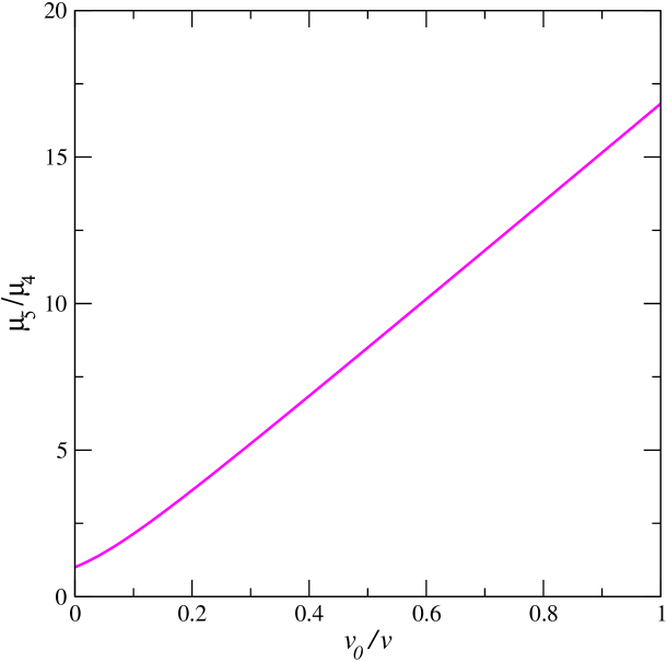
Figure 1: The minimum possible value of $\mu_{5}/\mu_{4}$ as a function of $v_{0}/v$.

It is seen that, unless $v_{0}$ is very small, the lighter pseudoscalar will in general be ten or more times lighter than the heavier pseudoscalar. But, $v_{0}$ cannot be too small, lest the Yukawa coupling responsible for the top-quark mass needs to be very large.

3.4 The eigenvectors in the limit $v_{1}=0$

As a preparation for the next section, we now investigate the limit $v_{1}=0$ in detail. In that limit $a_{4}$ and $\mu_{\mathrm{m}}$ must also vanish, hence the scalar mass matrices are given by

$$\mathcal{M}^{2}_{\varphi} = \frac{1}{2}\left(\begin{array}[]{ccc}-a_{3}v_{2}^{2}&0&a_{3}v_{0}v_{2}\\ 0&-a_{3}v_{0}^{2}+\left(a_{6}-2a_{5}\right)v_{2}^{2}&0\\ a_{3}v_{0}v_{2}&0&-a_{3}v_{0}^{2}\end{array}\right),$$ (94)

$$\mathcal{M}^{2}_{\rho} = \frac{1}{2}\left(\begin{array}[]{ccc}4a_{1}v_{0}^{2}&0&2Bv_{0}v_{2}\\ 0&Av_{2}^{2}&0\\ 2Bv_{0}v_{2}&0&4a_{5}v_{2}^{2}\end{array}\right),$$ (98)

$$\mathcal{M}^{2}_{\eta} = \frac{1}{2}\left(\begin{array}[]{ccc}0&0&0\\ 0&Av_{2}^{2}&0\\ 0&0&0\end{array}\right).$$ (102)

From the positivity of the mass matrices $\mathcal{M}^{2}_{\varphi}$ and $\mathcal{M}^{2}_{\rho}$ we then have

$$a_{3}<0\quad\mbox{and}\quad 4a_{1}a_{5}>\left(a_{2}+a_{3}\right)^{2},$$ (103)

respectively. Notice that $a_{1}$ and $a_{5}$ must be positive, even when $v_{1}\neq 0$, in order for the potential to have a minimum.

Equations (94)–(102) show that $\phi_{1}$ completely decouples from $\phi_{0}$ and $\phi_{2}$ in the limit $v_{1}=0$. In that limit one has

$$m_{2}^{2}=-\frac{a_{3}}{2}\,v_{0}^{2}+\left(\frac{a_{6}}{2}-a_{5}\right)v_{2}^{2},\quad\mu_{2}^{2}=\mu_{5}^{2}=\frac{A}{2}\,v_{2}^{2},\quad\mu_{4}^{2}=0,\quad Y_{2}=X_{2}=X_{5}=\left(\begin{array}[]{c}0\\ 1\\ 0\end{array}\right).$$ (104)

Moreover, equation (94) readily gives

$$m_{1}^{2}=-\frac{a_{3}}{2}\,v^{2},\quad Y_{1}=\frac{1}{v}\left(\begin{array}[]{c}-v_{2}\\ 0\\ v_{0}\end{array}\right).$$ (105)

while equation (98) leads to

$$\mu^{2}_{1,3}=a_{1}v_{0}^{2}+a_{5}v_{2}^{2}\pm\sqrt{\left(a_{1}v_{0}^{2}-a_{5}v_{2}^{2}\right)^{2}+B^{2}v_{0}^{2}v_{2}^{2}},$$ (106)

and

$$X_{1}=\left(\begin{array}[]{c}\cos\lambda\\ 0\\ -\sin\lambda\end{array}\right),\quad X_{3}=\left(\begin{array}[]{c}\sin\lambda\\ 0\\ \cos\lambda\end{array}\right),\quad\tan{2\lambda}=\frac{Bv_{0}v_{2}}{a_{5}v_{2}^{2}-a_{1}v_{0}^{2}}.$$ (107)

4 Phenomenology of the scalar sector

The aim of this section is to demonstrate that the model presented in this paper complies with all the experimental constraints. We remind the reader that the masses of the physical scalars, and the mixing angles contained in the eigenvectors $Y_{a}$ ($a=1,2$) and $X_{b}$ ($b=1,\ldots,5$), are functions of the scalar-potential quartic couplings $a_{1},\dots,a_{7}$ and of $v_{0}/v$. It is beyond the scope of this paper to perform a complete exploration of this large parameter space; we shall restrict ourselves to show that it is possible to find a set of parameters such that the scalar sector of the model does not contradict any experimental results. We will choose one such set and call it ‘the reference scenario’.

Although the present model is mainly designed for the lepton sector, one may extend it to the quark sector, as mentioned in section 3.1. The obvious way to do this is to stipulate that under the $\mathbbm{Z}_{2}$ symmetry in (5) the right-handed-quark gauge-$SU(2)$ singlets transform with a minus sign. Then, only $\phi_{0}$ has Yukawa couplings to the quark sector. In this way there are, just as in the SM, no flavour-changing neutral Yukawa interactions of the quarks. This extension resembles in its spirit a type-I two-Higgs-doublet model (2HDM). We require $v_{0}\>\mbox{\raisebox{-3.0pt}{$\stackrel{{\scriptstyle\displaystyle>}}{{\sim}}$}}\>100$ GeV in order to avoid a top-quark Yukawa coupling much larger than unity.

The Lagrangian for a generic multi-Higgs-doublet model (MHDM) can be found in [10].

4.1 Constraints from $Z^{0}$ decay

$Z^{0}$ decay into charged scalars

In a MHDM, the $Z^{0}$ couples to $S^{+}_{a}S^{-}_{a}$ with a universal strength, independent of the details of charged-scalar mixing; the relevant term in the Lagrangian is

$$\frac{ig\left(s_{W}^{2}-c_{W}^{2}\right)}{2c_{W}}\,Z_{\mu}\sum_{a}\left(S_{a}^{+}\partial^{\mu}S_{a}^{-}-S_{a}^{-}\partial^{\mu}S_{a}^{+}\right).$$ (108)

A model-independent lower bound on the masses $m_{a}$ of the charged scalars can be derived from the invisible decay width of the $Z^{0}$. Subtracting from it the SM decay width of the $Z^{0}$ into neutrinos, the difference is compatible with zero, leaving little room for an additional decay of the $Z^{0}$ into charged scalars [11]. This results in the bound [12]

$$m_{a}>43.7\ \mbox{GeV}\ \left(95\%\ \mbox{CL}\right),\ a=1,2.$$ (109)

Higgs strahlung

From LEP data, a lower mass limit $m_{h}>114.4$ GeV has been deduced [13] for the SM Higgs particle $h$, from the unobserved “Higgs strahlung” process $e^{+}e^{-}\to Z^{\ast}\to Zh$. Note that this process is allowed only for scalars but not for pseudoscalars [14]. In the present model, all three scalars $S^{0}_{1,2,3}$ can in principle be produced by Higgs strahlung; the relevant term in the Lagrangian is

$$\frac{gm_{Z}}{2c_{W}}\,Z_{\mu}Z^{\mu}\sum_{b=1}^{3}\left(X_{0}\cdot X_{b}\right)S^{0}_{b},$$ (110)

where the quantity in parentheses denotes the scalar products of the vectors $X_{0}$ and $X_{b}$. In the limit $v_{1}=0$ the production of $S^{0}_{2}$ is suppressed since $X_{0}\cdot X_{2}=0$, as can be read off from equations (57) and (104). On the other hand, in that limit the strengths of the couplings of $S^{0}_{1}$ and $S^{0}_{3}$ are complementary, with $\left(X_{0}\cdot X_{1}\right)^{2}+\left(X_{0}\cdot X_{3}\right)^{2}=1$.

Associated production

The $Z^{0}$ can decay into a scalar–pseudoscalar pair [14]; the relevant term in the Lagrangian is

$$\frac{g}{2c_{W}}\,Z_{\mu}\,\sum_{b=1}^{3}\sum_{b^{\prime}=4}^{5}\left(X_{b}\cdot X_{b^{\prime}}\right)\left(S_{b}^{0}\partial^{\mu}S_{b^{\prime}}^{0}-S_{b^{\prime}}^{0}\partial^{\mu}S_{b}^{0}\right).$$ (111)

The lightest pseudoscalar of our model, $S^{0}_{4}$, can in general be produced in this way associated with either $S^{0}_{1}$ or $S^{0}_{3}$, but not with $S^{0}_{2}$, since $X_{4}\cdot X_{2}=0$ in the limit of vanishing $v_{1}$.

4.2 Constraints from other decays

Decays of the charged scalars

The 2HDM has a single charged scalar $H^{+}$. Assuming $\mbox{BR}\left(H^{+}\to\tau^{+}\nu_{\tau}\right)+\mbox{BR}\left(H^{+}\to c\bar{s}\right)\simeq 1$, the bound $m_{H^{+}}>78.6$ GeV (95% CL) has been derived from the combined LEP data [13]. One cannot use this bound uncritically in the present model, which has two charged scalars and in which $\mbox{BR}\left(S_{a}^{+}\to\mu^{+}\nu_{\mu}\right)$ is certainly non-negligible. Still, the bound on $m_{H^{+}}$ suggests an estimate of how much the bound (109) can possibly be raised by taking into account specific decay channels of $S_{a}^{+}$.

Other decays

The transition $b\to s\gamma$ is important because it provides an indirect, yet quite stringent, lower bound on the charged-scalar masses [15]. Since only $\phi_{0}$ has Yukawa couplings to the quarks and the $S^{+}_{2}$ component of $\varphi^{+}_{0}$ is suppressed, the lower bound from $b\to s\gamma$ applies only to $m_{1}$. Vector mesons could possibly decay into a very light scalar plus a photon [18], yielding a lower bound on the scalar mass. This is relevant for the decay $\Upsilon\left(1S\right)\to S^{0}_{4}\gamma$. Loop corrections in the decay $Z^{0}\to\bar{b}b$ are also important [19] in the 2HDM for large $\tan\beta$. However, since our model has features similar to a 2HDM with $\tan\beta\sim 1$, in which range this decay is not stringent [16], we will disconsider it in the following.

4.3 “Safe” scalar masses

In the light of the above discussion we require

$$m_{1}\>\mbox{\raisebox{-3.0pt}{$\stackrel{{\scriptstyle\displaystyle>}}{{\sim}}$}}\>350\ \mbox{GeV},\quad\mu_{1}\>\mbox{\raisebox{-3.0pt}{$\stackrel{{\scriptstyle\displaystyle>}}{{\sim}}$}}\>120\ \mbox{GeV},\quad\mu_{3}\>\mbox{\raisebox{-3.0pt}{$\stackrel{{\scriptstyle\displaystyle>}}{{\sim}}$}}\>120\ \mbox{GeV},\quad\mu_{4}>10\ \mbox{GeV}.$$ (112)

Some remarks are at order. In the 2HDM of type II the bound on the charged-scalar mass from $b\to s\gamma$ is of the order of several hundred GeV, much larger than the bound from direct LEP searches. We have rather arbitrarily set that bound to 350 GeV in (112), by considering the results obtained in [15] for $\tan\beta\sim 1$ and taking into account the considerable uncertainty in the computation of the corresponding $B$-meson decay. The bounds on $\mu_{1}$ and $\mu_{3}$ have been stipulated in order to definitely avoid production via Higgs strahlung. Finally, the lower bound on $\mu_{4}$ stems from the wish to avoid any problems from $\Upsilon(1S)\to S^{0}_{4}\gamma$. We have not put lower bounds on $m_{2}$, $\mu_{2}$, and $\mu_{5}$ in (112) because, from the discussions in the previous paragraphs, we conclude that there are no really stringent bounds on these masses. Of course, these masses should not be too small. In any case, numerically it will turn out that if we fulfill the constraints of (112), then also $m_{2}$ and $\mu_{2}$ will be reasonably large. Moreover, we bear in mind that in our model $\mu_{5}\gg\mu_{4}$ holds anyway.

4.4 A reference scenario

In table 1 we have written down a set of values for the eight parameters of the model, which we define to be our ‘reference scenario’. All input values are of order one, except $a_{3}$ which is somewhat larger because it is responsible for a large mass $m_{1}$—see equation (105). In table 1, $|a_{4}|_{\mathrm{max}}=Av_{1}v_{2}/v_{0}^{2}$ is the maximal value of $|a_{4}|$, obtained from equation (20).

$v_{0}/v$	$a_{1}$	$a_{2}$	$a_{3}$	$\left|a_{4}\right|/\left|a_{4}\right|_{\mathrm{max}}$	$a_{5}$	$a_{6}$	$a_{7}$
$1/\sqrt{2}$	2.5	3	$-5$	0.4	1.5	2	3

Table 1: Input values for the reference scenario.

Taking the input from table 1 and performing a numerical calculation, we obtain

$$\begin{array}[]{lclclclclcl}m_{1}&=&389.2\ \mbox{GeV},&&m_{2}&=&245.8\ \mbox{GeV},\\ \mu_{1}&=&434.8\ \mbox{GeV},&&\mu_{2}&=&171.9\ \mbox{GeV},&&\mu_{3}&=&231.8\ \mbox{GeV},\\ \mu_{4}&=&14.3\ \mbox{GeV},&&\mu_{5}&=&173.8\ \mbox{GeV}.&&&\end{array}$$ (113)

These values agree well with the ones computed from the approximate formulae of section 3.4. For instance, $\mu_{2}\simeq\mu_{5}$ in (113). The masses (113) satisfy the conditions (112) for “safe” masses.

Next we check the reference scenario against electroweak precision data by using the oblique parameters [20] $S$, $T$, and $U$. For a MHDM we take the formula for $T$ in [10] (for computations of $T$ in the 2HDM, see e.g. [14, 22, 23]), which gives, when applied to the present model

$$T = \frac{1}{16\pi s_{W}^{2}m_{W}^{2}}\left\{\sum_{a=1}^{2}\sum_{b=1}^{5}\left(Y_{a}\cdot X_{b}\right)^{2}F\left(m_{a}^{2},\,\mu_{b}^{2}\right)\right.$$ (114)

$$-\sum_{b=1}^{3}\sum_{b^{\prime}=4}^{5}\left(X_{b}\cdot X_{b^{\prime}}\right)^{2}F\left(\mu_{b}^{2},\,\mu_{b^{\prime}}^{2}\right)$$

$$+3\sum_{b=1}^{3}\left(X_{0}\cdot X_{b}\right)^{2}\left[F\left(m_{Z}^{2},\,\mu_{b}^{2}\right)-F\left(m_{W}^{2},\,\mu_{b}^{2}\right)\right]$$

$$\left.-3\left[F\left(m_{Z}^{2},\,m_{h}^{2}\right)-F\left(m_{W}^{2},\,m_{h}^{2}\right)\right]\vphantom{\sum_{a=1}^{2}\sum_{b=1}^{5}}\right\},$$

where

$$F\left(x,\,y\right)=\frac{x+y}{2}-\frac{xy}{x-y}\,\ln{\frac{x}{y}}.$$ (115)

In equation (114), $m_{W}$ and $m_{Z}$ are the masses of the $W^{\pm}$ and $Z^{0}$ gauge bosons, respectively, $s_{W}^{2}=1-m_{W}^{2}/m_{Z}^{2}$, and $m_{h}$ is the mass of the SM Higgs boson. One may also write down formulae for $S$ and for $U$ by applying the results in [21]. Taking the central value $m_{h}=87$ GeV from recent SM fits [24] and using the scalar masses and diagonalizing matrices of the reference scenario, we have obtained $S=0.046$, $T=-0.162$, and $U=-0.002$. These values are compatible with the fit results for the oblique parameters given in [25]. We note that, while all the individual contributions to $S$ and to $U$ are small and no excessive cancellations occur among them, this is not so for $T$: considering separately the first and the second terms in the right-hand side (RHS) of equation (114), each of them is one order of magnitude larger than the final result $T=-0.162$; however, those two contributions have opposite signs (note that $F\geq 0$), leading to a partial cancellation. Nevertheless, a certain amount of tuning of the input parameters is expedient to achieve the correct order of magnitude of $T$, as will be discussed in the next paragraph. The numerical value of third term of the RHS of equation (114) is naturally one order of magnitude smaller than the values of the first and second terms, and the SM subtraction in the forth term is numerically a tiny effect.

In figure 2

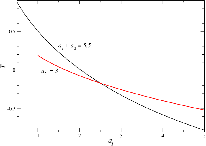
Figure 2: The oblique parameter $T$ as a function of $a_{1}$. The input parameters not shown in the plot are as in table 1.

we have attempted to illustrate the dependence of $T$ on the input parameters $a_{1}$ and $a_{2}$; these occur only in the mass matrix of the neutral scalars (49) and might, therefore, be able to disturb the cancellation between the first and second terms in the RHS in equation (114). In figure 2 we have plotted two curves. In the first one we have fixed $a_{2}=3$ to its value in the reference scenario, whereas in the other one we have fixed $a_{1}+a_{2}=5.5$; the crossing point of the curves corresponds to the reference scenario. The figure illustrates nicely the tuning required for keeping $T$ small. We note that the curve with fixed $a_{2}$ begins at $a_{1}=1$, where $\mu_{3}=115$ GeV is outside the region of “safe” masses, but $\mu_{3}$ quickly grows with $a_{1}$.

5 Conclusions

In this paper we have presented a model for the lepton sector based on the family symmetry $O(2)$. The model has an obvious extension to the quark sector, by coupling to the quarks only the Higgs doublet $\phi_{0}$ which transforms trivially under $O(2)$. The smallness of the masses of the light neutrinos is explained in our model through the seesaw mechanism. The reflection symmetry contained in $O(2)$ acts as a $\mu$–$\tau$ interchange symmetry, which—together with the $U(1)\subset O(2)$—enforces diagonal Yukawa-coupling matrices and a neutrino mass matrix of the form (1). Consequently, the model predicts $\theta_{23}=\pi/4$ and $\theta_{13}=0$ at the tree level. In that respect the model in this paper is practically identical to the one in [7]; in both models the lepton flavour violation resides only in the mass matrix of the right-handed neutrinos. It has been shown [26] that models of this class are safe from flavour-changing neutral interactions.

The crucial difference between the present model and the one in [7] is that, in the $O(2)$ model, we allow a non-trivial transformation of the Higgs doublets $\phi_{1}$ and $\phi_{2}$ under the $U(1)\subset O(2)$. In this way, we obtain a relation between the smallness of the mass ratio $m_{\mu}/m_{\tau}$ and the small mass $\mu_{4}$ of one of the two pseudoscalars of the model; indeed, that pseudoscalar is almost a Goldstone boson and only a soft $U(1)$ breaking in the scalar potential prevents $\mu_{4}$ from being exactly zero. On the other hand, that soft breaking must necessarily be small in order to reproduce the small value of $m_{\mu}/m_{\tau}=v_{1}/v_{2}$, determined by the ratio of the VEVs of $\phi_{1}$ and $\phi_{2}$.

It had previously been realized [16, 27] that, in the 2HDM, one of the neutral scalars could be quite light without contradicting any experimental constraints. We have attempted to show that the same holds in our three-Higgs-doublet model. Actually, our model not only predicts the light pseudoscalar, it also predicts the near equality of the mass of one of the scalars and the mass of the heaviest pseudoscalar, and, in addition, specific features in scalar mixing, resulting from the near decoupling of $\phi_{1}$ from $\phi_{0}$ and $\phi_{2}$, due to the smallness of $m_{\mu}/m_{\tau}$. We have thus demonstrated that, within our $O(2)$ model, the connection between the lepton and scalar sectors can be much tighter than usually thought of.

Appendix A The group $O(2)$

Definition and characterization

$O(2)$ is the group of rotations and reflections of the plane. It is generated by rotations $g\left(\theta\right)$, with angle $\theta$, around the center of the coordinate system, and by the reflection $s$ about the $x$-axis. Allowing the angle $\theta$ to vary over $\mathbbm{R}$, the properties of these group elements, which fully characterize the group, are

$$g\left(\theta+2\pi\right)=g\left(\theta\right),\quad g\left(\theta_{1}\right)g\left(\theta_{2}\right)=g\left(\theta_{1}+\theta_{2}\right),\quad s^{2}=e,\quad s\,g\left(\theta\right)s=g\left(-\theta\right).$$ (A1)

Irreducible representations

There are two singlet irreducible representations of $O(2)$:

$$\underline{1}:\ g\left(\theta\right)\to 1,\ s\to 1\quad\mbox{and}\quad\underline{1}^{\prime}:\ g\left(\theta\right)\to 1,\ s\to-1.$$ (A2)

Furthermore, $O(2)$ has a countably infinite set of doublet irreducible representations, numbered by $n\in\mathbbm{N}$:

$$\underline{2}^{(n)}:\ g\left(\theta\right)\to\left(\begin{array}[]{cc}e^{in\theta}&0\\ 0&e^{-in\theta}\end{array}\right),\ s\to\left(\begin{array}[]{cc}0&1\\ 1&0\end{array}\right).$$ (A3)

Tensor product $\underline{2}^{(m)}\otimes\underline{2}^{(n)}$

We assume that the matrices in (A3) act on an orthonormal basis $\{e_{1},\,e_{2}\}$. In the product $\underline{2}^{(m)}\otimes\underline{2}^{(n)}$ we must distinguish two cases. If $m>n$, then

$$\underline{2}^{(m)}\otimes\underline{2}^{(n)}=\underline{2}^{(m+n)}\oplus\underline{2}^{(m-n)}.$$ (A4)

The irreducible representations in the right-hand side of (A4) have basis vectors

$$\underline{2}^{(m+n)}:\ e_{1}\otimes e_{1},\ e_{2}\otimes e_{2}\quad\mbox{and}\quad\underline{2}^{(m-n)}:\ e_{1}\otimes e_{2},\ e_{2}\otimes e_{1}.$$ (A5)

If $m=n$, then

$$\underline{2}^{(n)}\otimes\underline{2}^{(n)}=\underline{1}\oplus\underline{1}^{\prime}\oplus\underline{2}^{(2n)}.$$ (A6)

The irreducible representations in the right-hand side of (A6) have basis vectors

$$\underline{1}:\ \frac{1}{\sqrt{2}}\left(e_{1}\otimes e_{2}+e_{2}\otimes e_{1}\right),\quad\underline{1}^{\prime}:\ \frac{1}{\sqrt{2}}\left(e_{1}\otimes e_{2}-e_{2}\otimes e_{1}\right),\quad\underline{2}^{(2n)}:\ e_{1}\otimes e_{1},\ e_{2}\otimes e_{2}.$$ (A7)

Appendix B Comparison of the present model with the model of softly broken lepton numbers

The $\mathbbm{Z}_{2}$ model

The model presented in this paper—let us call it “$O(2)$ model”—is quite similar to the model proposed by two of us a few years ago [7]—let us call it “$\mathbbm{Z}_{2}$ model”. The $\mathbbm{Z}_{2}$ model has the same fermion and scalar multiplets as the $O(2)$ model. Both the $\mathbbm{Z}_{2}$ and $O(2)$ models have the $s$ of (2) and the $\mathbbm{Z}_{2}$ of (5) as symmetries. However, instead of the $U(1)$ of (4), employed as a symmetry in the $O(2)$ model, the $\mathbbm{Z}_{2}$ model requires the conservation, in all terms of dimension four in the Lagrangian, of the three family lepton numbers. As a consequence, the Yukawa Lagrangian of the $\mathbbm{Z}_{2}$ model has, beyond the terms in equation (7), one further term:

$$\mathcal{L}_{Y}=\cdots-y_{5}\left(\bar{D}_{\mu L}\phi_{2}\mu_{R}+\bar{D}_{\tau L}\phi_{1}\tau_{R}\right)+\mbox{H.c.}$$ (B1)

Therefore, in the $\mathbbm{Z}_{2}$ model the ratio between the muon and tau masses is

$$\frac{m_{\mu}}{m_{\tau}}=\left|\frac{y_{4}v_{1}+y_{5}v_{2}}{y_{4}v_{2}+y_{5}v_{1}}\right|.$$ (B2)

Symmetry group $O(2)$ in the $\mathbbm{Z}_{2}$ model

It was noted as a side remark in [28] that the $\mathbbm{Z}_{2}$ model also has family symmetry $O(2)$. This group $O(2)$ is generated by the $\mu$–$\tau$ interchange symmetry $s$ together with the $U(1)$ of the lepton number $L_{\mu}-L_{\tau}$. Replacing $\phi_{1}$ and $\phi_{2}$ by $\phi_{\pm}\equiv\left(\phi_{1}\pm\phi_{2}\right)\left/\sqrt{2}\right.$, we see that, under that $O(2)$, $\phi_{+}$ transforms as a $\underline{1}$ and $\phi_{-}$ as a $\underline{1}^{\prime}$. The $O(2)$ model, on the other hand, has two Higgs doublets transforming as a $\underline{2}^{(2)}$ of $O(2)$, instead of as a $\underline{1}\oplus\underline{1}^{\prime}$; one further difference is that the $U(1)$ group in the $O(2)$ model is not really $L_{\mu}-L_{\tau}$, cf. (4).

Naturally small $m_{\mu}/m_{\tau}$ in the $\mathbbm{Z}_{2}$ model

In [8] an additional symmetry, dubbed $K$, was introduced into the $\mathbbm{Z}_{2}$ model in order to provide a technically natural explanation for the smallness of $m_{\mu}/m_{\tau}$. Under $K$, $\phi_{1}$ and $\mu_{R}$ change sign while all other fields remain invariant. The symmetry $K$ eliminates the $y_{5}$ term—see equation (B1)—from the Yukawa Lagrangian of the $\mathbbm{Z}_{2}$ model, thus obtaining $m_{\mu}/m_{\tau}=\left|v_{1}/v_{2}\right|$ just as in the $O(2)$ model. We want to stress that, from the point of view of neutrino masses and lepton mixing, the $O(2)$ model of the present paper is equivalent to the $\mathbbm{Z}_{2}$ model of [7] and also to the $\mathbbm{Z}_{2}$ model with the additional symmetry $K$ of [8]. The difference lies in the scalar potential, which in the $O(2)$ model is both different and more restricted. Indeed, in the $\mathbbm{Z}_{2}$ model with a softly broken symmetry $K$, the $a_{4}$ term is absent from the scalar potential; on the other hand, there are extra terms

$$V=\cdots+b_{1}\left[\left(\phi_{1}^{\dagger}\phi_{2}\right)^{2}+\left(\phi_{2}^{\dagger}\phi_{1}\right)^{2}\right]+\left\{b_{2}\left[\left(\phi_{0}^{\dagger}\phi_{1}\right)^{2}+\left(\phi_{0}^{\dagger}\phi_{2}\right)^{2}\right]+\mbox{H.c.}\right\},$$ (B3)

with $b_{1}$ real but $b_{2}$ in general complex. The model of [8] has the advantage, over the $O(2)$ model, that $m_{\mu}/m_{\tau}$ is small in a technically natural sense; indeed, in that model $v_{1}\neq 0$ only obtains when $K$ is softly broken by the $\mu_{3}$ term, while in the $O(2)$ model $v_{1}\neq 0$, even if $\mu_{3}=0$, because of the $a_{4}$ term. The advantage of the $O(2)$ model is its prediction of a light pseudoscalar—a prediction inexistent in the model of [8].

Appendix C Substitution of the symmetry $s$ by a non-diagonal $CP$ symmetry

In the model suggested in this paper it is possible to use, instead of the $\mu$–$\tau$ interchange symmetry $s$, the non-trivial $CP$ symmetry [9, 29]

$$CP:\left\{\begin{array}[]{rcl}D_{\alpha L}&\to&iS_{\alpha\beta}\gamma^{0}C\bar{D}_{\beta L}^{T},\\ \alpha_{R}&\to&iS_{\alpha\beta}\gamma^{0}C\bar{\beta}_{R}^{T},\\ \nu_{\alpha R}&\to&iS_{\alpha\beta}\gamma^{0}C\bar{\nu}_{\beta R}^{T},\\ \phi_{0}&\to&\phi_{0}^{\ast},\\ \phi_{1}&\to&\phi_{2}^{\ast},\\ \phi_{2}&\to&\phi_{1}^{\ast},\end{array}\right.\quad\mbox{where}\ S=\left(\begin{array}[]{ccc}1&0&0\\ 0&0&1\\ 0&1&0\end{array}\right)$$ (C1)

and $C$ is the Dirac–Pauli charge conjugation matrix. This $CP$ symmetry commutes with both the $U(1)$ of (4) and the $\mathbbm{Z}_{2}$ of (5), so that, in this case, the model has symmetry $CP\times U(1)\times\mathbbm{Z}_{2}$ instead of $O(2)\times\mathbbm{Z}_{2}$. Instead of equation (7) we would then have

$$\mathcal{L}_{Y} = -y_{1}\,\bar{D}_{eL}\tilde{\phi}_{0}\nu_{eR}-\left(y_{2}\,\bar{D}_{\mu L}\tilde{\phi}_{0}\nu_{\mu R}+y_{2}^{\ast}\,\bar{D}_{\tau L}\tilde{\phi}_{0}\nu_{\tau R}\right)$$ (C2)

$$-y_{3}\,\bar{D}_{eL}\phi_{0}e_{R}-\left(y_{4}\,\bar{D}_{\mu L}\phi_{1}\mu_{R}+y_{4}^{\ast}\,\bar{D}_{\tau L}\phi_{2}\tau_{R}\right)+\mbox{H.c.,}$$

with real $y_{1,3}$. We would end up with [30]

$$\mathcal{M}_{\nu}=\left(\begin{array}[]{ccc}x&y&y^{\ast}\\ y&z&w\\ y^{\ast}&w&z^{\ast}\end{array}\right)$$ (C3)

$x$ and $w$ being real. Such a model predicts [9] maximal atmospheric-neutrino mixing ($\theta_{23}=\pi/4$) but, instead of $U_{e3}=0$, it predicts [2, 9] $\left|U_{\mu i}\right|=\left|U_{\tau i}\right|$ for all $i=1,2,3$ ($U$ is the lepton mixing matrix), which leads to $\sin{\theta_{13}}\cos{\delta}=0$, with $\delta$ being the $CP$-violating phase in the mixing matrix. Although this condition permits $\theta_{13}=0$, it can be shown that the more general case is that of maximal $CP$ violation [9] i.e. $\delta=\pm\pi/2$. The scalar potential is the same as in equation (13) with the proviso (14).

References

-
[1]
T. Fukuyama and H. Nishiura,
Mass matrix of Majorana neutrinos,
hep-ph/9702253;
E. Ma and M. Raidal, Neutrino mass, muon anomalous magnetic moment, and lepton flavor nonconservation, Phys. Rev. Lett. 87 (2001) 011802 [hep-ph/0102255]; [erratum ibid. 87 (2001) 159901];
C.S. Lam, A 2–3 symmetry in neutrino oscillations, Phys. Lett. B 507 (2001) 214 [hep-ph/0104116];
K.R.S. Balaji, W. Grimus and T. Schwetz, The solar LMA neutrino oscillation solution in the Zee model, Phys. Lett. B 508 (2001) 301 [hep-ph/0104035];
E. Ma, The all-purpose neutrino mass matrix, Phys. Rev. D 66 (2002) 117301 [hep-ph/0207352]. - [2] P.F. Harrison and W.G. Scott, – reflection symmetry in lepton mixing and neutrino oscillations, Phys. Lett. B 547 (2002) 219 [hep-ph/0210197].
- [3] For additional references see H. Nishiura, K. Matsuda and T. Fukuyama, Quark mixing from mass matrix model with flavor , arXiv:0804.4515.
-
[4]
M. Maltoni, T. Schwetz, M.A. Tórtola and J.W.F. Valle,
Status of global fits to neutrino oscillations,
New J. Phys. 6 (2004) 122
[hep-ph/0405172];
G.L. Fogli, E. Lisi, A. Marrone and A. Palazzo, Global analysis of three-flavor neutrino masses and mixings, Prog. Part. Nucl. Phys. 57 (2006) 742 [hep-ph/0506083];
T. Schwetz, Global fits to neutrino oscillation data, Phys. Scripta T127 (2006) 1 [hep-ph/0606060]. -
[5]
P. Minkowski,
at a rate of one out of muon decays?,
Phys. Lett. B 67 (1977) 421;
T. Yanagida, Horizontal gauge symmetry and masses of neutrinos, in Proceedings of the workshop on unified theory and baryon number in the universe (Tsukuba, Japan, 1979), O. Sawata and A. Sugamoto eds., KEK report 79-18, Tsukuba, 1979;
S.L. Glashow, in Quarks and leptons, proceedings of the advanced study institute (Cargèse, Corsica, 1979), J.-L. Basdevant et al. eds., Plenum, New York, 1981;
M. Gell-Mann, P. Ramond and R. Slansky, Complex spinors and unified theories, in Supergravity, D.Z. Freedman and F. van Nieuwenhuizen eds., North Holland, Amsterdam, 1979;
R.N. Mohapatra and G. Senjanović, Neutrino mass and spontaneous parity violation, Phys. Rev. Lett. 44 (1980) 912. - [6] E. Ma, Two derivable relationships among quark masses and mixing angles, Phys. Rev. D 43 (1991) R2761.
- [7] W. Grimus and L. Lavoura, Softly broken lepton numbers and maximal neutrino mixing, J. High Energy Phys. 07 (2001) 045 [hep-ph/0105212]; Softly broken lepton numbers: an approach to maximal neutrino mixing, Acta Phys. Polonica B 32 (2001) 3719 [hep-ph/0110041].
- [8] W. Grimus and L. Lavoura, Maximal atmospheric neutrino mixing and the small ratio of muon to tau mass, J. Phys. G: Nucl. Part. Phys. 20 (2004) 73 [hep-ph/0309050].
- [9] W. Grimus and L. Lavoura, A non-standard transformation leading to maximal atmospheric neutrino mixing, Phys. Lett. B 579 (2004) 113 [hep-ph/0305309].
- [10] W. Grimus, L. Lavoura, P. Osland and O.M. Ogreid, A precision constraint on multi-Higgs-doublet models, arXiv:0711.4022 [hep-ph].
- [11] J. Abdallah et al. (DELPHI Collaboration), Search for charged Higgs bosons at LEP in general two Higgs doublet models, Eur. Phys. J. D 24 (2004) 399 [hep-ex/0404012].
- [12] ALEPH, DELPHI, L3, OPAL, SLD Collaborations, LEP Electroweak Working Group, SLD Electroweak and Heavy Flavour Groups, Precision electroweak measurements on the resonance, Phys. Rep. 427 (2006) 257. [hep-ex/0509008].
- [13] W.-M. Yao et al. (Particle Data Group), Review of particle physics, J. Phys. G: Nucl. Part. Phys. 33 (2006) 1.
- [14] J.F. Gunion, H.E. Haber, G.L. Kane and S. Dawson, The Higgs hunter’s guide, Addision–Wesley Publishing Company, Reading (Massachusetts) 1989.
-
[15]
A.J. Buras, M. Misiak, M. Münz and S. Pokorski,
Theoretical uncertainties
and phenomenological aspects of decay,
Nucl. Phys. B 424 (1994) 374
[hep-ph/9311345];
P. Gambino and M. Misiak, Quark mass effects in , Nucl. Phys. B 611 (2001) 338 [hep-ph/0104034];
M. Neubert, Renormalization-group improved calculation of branching ratio, Eur. Phys. J. C 40 (2005) 165 [hep-ph/0408179]. - [16] P.H. Chankowski, M. Krawczyk and J. Żochowski, Implications of the precision data for very light Higgs boson scenarios in 2HDM(II), Eur. Phys. J. C 11 (1999) 661 [hep-ph/9905436].
- [17] K. Cheung and O.C.W. Kong, Can the two-Higgs-doublet model survive the constraint from the muon anomalous magnetic moment?, Phys. Rev. D 68 (2003) 053003.
- [18] F. Wilczek, Decays of heavy vector mesons into Higgs particles, Phys. Rev. Lett. 39 (1977) 1304.
- [19] A. Denner, R.J. Guth, W. Hollik and J.K. Kühn, The Z-width in the two Higgs doublet model, Z. Phys. C 51 (1991) 695.
-
[20]
B.W. Lynn, M.E. Peskin, and R.G. Stuart,
in Physics at LEP,
J. Ellis and R.D. Peccei eds. (CERN, Geneva, 1986);
D.C. Kennedy and B.W. Lynn, Electroweak radiative corrections with an effective Lagrangian: Four-fermion processes, Nucl. Phys. B 322 (1989) 1;
M.E. Peskin and T. Takeuchi, A new constraint on a strongly interacting Higgs sector, Phys. Rev. Lett. 65 (1990) 964;
G. Altarelli and R. Barbieri, Vacuum-polarization effects of new physics on electroweak processes, Phys. Lett. B 253 (1991) 161;
M.E. Peskin and T. Takeuchi, Estimation of oblique electroweak corrections, Phys. Rev. D 46 (1992) 381.
G. Altarelli, R. Barbieri, and S. Jadach, Toward a model-independent analysis of electroweak data, Nucl. Phys. B 369 (1992) 3 [erratum ibid. B 376 (1992) 444];
I. Maksymyk, C.P. Burgess, and D. London, Beyond S, T, and U, Phys. Rev. D 50 (1994) 529 [hep-ph/9306267]. - [21] W. Grimus, L. Lavoura, P. Osland and O.M. Ogreid, The oblique parameters in multi-Higgs-doublet models, arXiv:0802.4353 [hep-ph].
- [22] S. Bertolini, Quantum effects in a two-Higgs-doublet model of the electroweak interactions, Nucl. Phys. B 272 (1986) 77.
- [23] A.W. El Kaffas, W. Khater, O.M. Ogreid and P. Osland, Consistency of the two Higgs doublet model and violation in top production at the LHC, Nucl. Phys. B 775 (2007) 45 [hep-ph/0605142].
- [24] LEP-EWWG, http://www.cern.ch/LEPEWWG.
- [25] J. Erler and P. Langacker, in [13], p. 119.
- [26] W. Grimus and L. Lavoura, Soft lepton-flavor violation in a multi-Higgs-doublet seesaw model, Phys. Rev. D 66 (2002) 014016 [hep-ph/0204070].
- [27] M. Krawczyk and D. Temes, Large 2HDM(II) one-loop corrections in leptonic tau decays, Eur. Phys. J. C 44 (2005) 435 [hep-ph/0410248].
- [28] W. Grimus and L. Lavoura, Maximal atmospheric neutrino mixing in an model, Eur. Phys. J. C 28 (2003) 123. [hep-ph/0211334].
- [29] W. Grimus and L. Lavoura, Models of maximal atmospheric neutrino mixing, Acta Phys. Polonica B 34 (2003) 5393 [hep-ph/0310050].
- [30] K.S. Babu, E. Ma and J.W.F. Valle, Underlying symmetry for the neutrino mass matrix and the quark mixing matrix, Phys. Lett. B 552 (2003) 207 [hep-ph/0206292].