Collaborate, compete and share

Abstract

We introduce and study a model of an interacting population of agents who collaborate in groups which compete for limited resources. Groups are formed by random matching agents and their worth is determined by the sum of the efforts deployed by agents in group formation. Agents, on their side, have to share their effort between contributing to their group’s chances to outcompete other groups and resource sharing among partners, when the group is successful. A simple implementation of this strategic interaction gives rise to static and evolutionary properties with a very rich phenomenology. A robust emerging feature is the separation of the population between agents who invest mainly in the success of their group and agents who concentrate in getting the largest share of their group’s profits.

1 Introduction

The collective behavior of a population of interacting individuals often exhibits surprising properties, which can hardly be anticipated on the basis of the micro-economic interaction. Game theory provides a unified background for analyzing the outcomes of strategic interactions among individuals rationally pursuing their self-interestrubinstein94 . Its predictions, however, are often contradicted by empirical and experimental research already in simple cases such as the prisoner’s dilemma or the ultimatum game prisoner ; guth82 ; nowak00 . This casts even more serious doubts on its validity in cases where individuals face a more complex strategic problem, involving a large number of other agents, uncertainty and limited information. On the other hand, many collective phenomena in the natural sciences owe their peculiarity to laws of statistical nature rather than to their specific microscopic details. This suggests that an approach similar to that of statistical physics can complement the game theoretic approach and highlight the role of statistical laws in collective socio-economic phenomena. Much work has been done along these lines on models of socio-dynamicscastellano08 and on simple models of evolutionary dynamics nowak06 ; szabo07 . For example, in spite of the doom predictions of game theory on the inevitability of defective behavior in contexts such as the prisoners dilemma, a different approach has shown that cooperative behavior and altruism can indeed be sustained in a complex interactive environment, in several ways nowak06b .

Here we pursue this approach in a case where competition and the needs to cooperate are intertwined in the strategic interaction. Our setup is one where agents have to match in small groups, which compete for limited resources. Agents in those groups which succeed in this competition face the additional problem of sharing the profits among themselves. Agents have to decide how to divide their effort in either contributing to the success of their group or, when their group is successful, in securing the largest share of the group’s profit for themselves. A concrete example of this is public funding of academic research, for which empirical analyses start to appear barber06 . Individual researchers form networks which submit proposals for a specific call in their field. Only the best proposals get accepted. Once a particular proposal is accepted the funds (and the workload) are shared among the network partners. Each researcher may decide to either commit a large effort to the preparation of projects, which implies little effort in the negotiation stage if the project is approved, or to commit a limited effort, thus ensuring a larger profit when funds are to be divided but also making the whole project weaker. This set up combines the incentives to free ride inside the group with the necessity of cooperating with group members in order to out-compete other groups. The former is akin to incentives to defection in prisoner’s dilemma or ultimatum games, whereas the latter is typical of competitive behavior in markets, which is often conducive to efficient outcomes (optimal resource allocation). Does the tension between these two elements leads to virtuous or collusive behavior? This is the key issue we address here.

We shall focus on a model which offers a simple realization of the generic setup discussed above. This will not allow us to derive a general answer to the question above, but rather illustrates the complexity, i.e. the richness of behaviors, which lies behind it. Still, by extending our basic model in several directions, we shall be able to argue that our results are quite robust with respect to simple modifications of the model.

The paper is organized as follows. In Sec. 2 we introduce two versions of a simple model and discuss their behavior when agents have fixed strategies. The rest of the paper is focused on the second version of the model (two-stage game). The constraint of fixed strategies is lifted in Sec. 3, where the complicated phenomenology induced by imperfect imitation is described. The possibility for agents to mutate (i.e. to adopt a totally new strategy) is introduced and studied in Sec. 4. The effects of the variation of some features of the model are described in Sec. 5. Finally Sec. 6 presents some conclusions.

2 The model

Let us first introduce an extremely simple model (possibly the simplest) that describes the problem we are interested in. Simple considerations about its phenomenology lead to the formulation of a slightly more complicated model, that will be investigated in the rest of the paper.

We consider the cooperation of $N$ agents to develop a scientific project and the subsequent negotiation stage to share the awarded grant. Each project involves $N_{p}=2$ partners. At each time step every agent participates to one and only one project. There are hence $P=N/N_{p}=N/2$ projects. Each agent is endowed at each time step with a total amount of effort equal to 1 that he has to divide in two parts:

• A fraction $0\leq E_{i}\leq 1$ is used for the development of the project.

• A fraction $1-E_{i}$ is used for the negotiation process to share the grant awarded to the project.

At each time step agents are paired randomly and the resulting projects are ranked depending on their quality, measured by $E_{p}$, the sum of the energies devoted by participants to its development. $E_{p}$ will then be smaller than $2$ (smaller than $N_{p}$ in the general case). The $P_{0}$ projects with highest $E_{p}$ are financed with one unit of payoff. Others are not financed, i.e. they do not get any payoff. The threshold energy $E_{s}$ is the value of $E_{p}$ of the last project financed. In the case that several projects have the same energy equal to $E_{s}$ a random selection among them is performed. Unless specified otherwise we will always take $P_{0}=P/2$.

Participants to successful projects negotiate then the division of the grant awarded. The assumption is that the share they receive is proportional to effort they have not spent in the development of the project, that is

$$\frac{1-E_{i}}{2-E_{p}},~{}~{}~{}~{}E_{p}=\sum_{j\in p}E_{j},$$ (1)

where the sum over $j\in p$ includes all participants to the project $p$. It is clear that there are (at least in principle) opposite drives for each agent: is it better to maximize the probability of success of the project (taking $E_{i}$ large) or the share obtained if the project is successful (taking $E_{i}$ small)? As we shall see, much depends on the inter-temporal structure of the game.

2.1 One stage game

It is relatively easy to understand that if each round is considered independently then the best strategy of agents is to devote all their efforts to proposing good projects if we consider the usual assumptions of Game Theory about rationality of agents.

In order to see this, let us observe that the outcome of the game for an agent with strategy $E$, and in particular his expected payoff $\pi(E)$ depends on the distribution $f(E)$ of the energies of all the others. Assuming such distribution to be fixed, it is easy to derive exactly, in the $N=\infty$ limit, the threshold effort $E_{s}$, i.e. the minimal effort for a project to be financed, and using such a value, the probability $P^{\#}(E)$ for a single agent to be financed. In turn, this allows to compute the payoff $\pi(E)$.

Without entering into details, it is clear that if the threshold effort $E_{s}$ is larger than 1, agents with effort $E<E_{s}-1$ have no chance to participate to a successful project, hence their success probability and expected payoff will be strictly zero. On the other hand, if $E_{s}<1$, “zealous” agents with $E>E_{s}$ will always have their projects approved, independently on the effort of their partner. Similar arguments suggest that, for a generic distribution $f(E)$, the maximum expected payoff occurs for intermediate values $\bar{E}$ of the effort: a careful balance between work and negotiation is better than the extreme strategies $E=0$ and $E=1$. Indeed the former will too often fail to have their project approved whereas the latter will derive very little benefits from the projects they take part in. If there is a best strategy $\bar{E}$, then all agents will adopt it, suggesting that $f(E)$ should be sharply peaked around $\bar{E}$. In this situation, it is clear that agents having a slightly larger value of the effort $E=\bar{E}+\zeta$ (with $\zeta$ small enough) will have a larger chance of getting the project through without paying too much in the sharing phase, unless $\bar{E}=1$. Therefore, the situation with all agents choosing strategy $E=1$ is the unique Nash Equilibrium of the game. In other words, if agents can modify their strategies according to a sensible evolutionary dynamics nowak06 they will converge to this virtuous asymptotic state.

This strategy is an Evolutionary Stable State: if everyone has $E=1$, that is also the best strategy and no other strategy can invade it. It is also, in practice, an invading strategy itself, as in Ref. nowak90 , if we extend in a reasonable way the concept to our game: any possible starting condition will tend toward this state. In the one-stage setting, agents are then expected to converge to a simple symmetric equilibrium. Numerical simulations confirm this expectation.

2.2 Two stages game

One unsatisfactory aspect of the discussion above is that agents who are not financed stay idle and waste the effort $1-E$ they intended to spend in the negotiation process. This might not be realistic in many contexts. For this reason, we shall now move to a modified model based on the idea that an agent that is not busy with an accepted project will use all his effort in preparing the next one. More in detail, the duration of a project spans now two temporal units, as in overlapping generation models OLG : projects which are “prepared” in time step $t$ are “run” at time $t+1$. So at each time there is a batch of projects which agents prepare for the next period, and the previous batch of projects the best of which are operational. From the agents’ viewpoint, each has to share his unit of effort between preparing new projects and sharing the profits, if they are engaged in successful ones (Fig. 1). The key difference with the model above is that agents whose projects were not financed in the previous step are not involved in any negotiation, so they can use their whole effort endowment for the preparation of the next project (this is somehow similar to the War of Attrition game with implicit time cost as in Ref. eriksson04 , where the cost of waiting is just the inability to join other games). Therefore the effort $E^{\rm eff}_{i}$ available to an agent for working at time $t+1$ is equal to $E_{i}$ or $1$ depending on whether at time $t$ his project was financed or not.

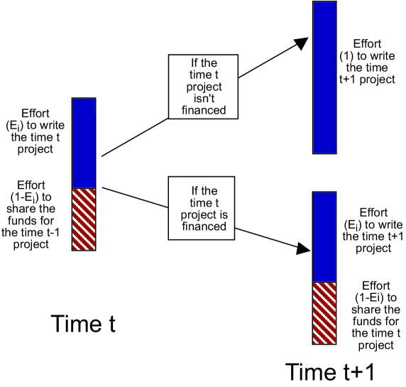
Figure 1: Schematic representation of the division of the total effort of an agent in the two stages game.

It is immediately clear that, at odds with what occurred in the one-stage game, no value of $E$ is too low for an agent to enter financed projects, because the unit effort available to an agent after a failure gives him good chances of being successful at the next step. This consideration intuitively leads to the expectation that there will be basically two potentially favorable strategies: either work always hard, have many financed projects and yield during the sharing process (finite $E$) or work hard only every second project, have only half of the projects financed but get as much as you can out of these (vanishing $E$).

Indeed, if the effort distribution function $f(E)$ is fixed, the expected payoff $\pi(E)$ has two peaks, as shown in Fig. 2 for a representative example.

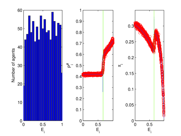
Figure 2: Behavior of the success probability $P^{\#}_{i}$ and of the payoff $\pi_{i}$ for the agent $i$ (following strategy $E_{i}$) for a fixed effort distribution $f(E)=1$; the blue lines are the expected values (as computed in the Appendix), the green vertical lines denote $E_{s}-1$.

For $E>E_{s}-1$ agents have a finite chance of being financed even if they have been financed the time before. For $E<E_{s}-1$ instead, agents can participate to a successful project only when their effective effort is 1, i.e. they have not been financed immediately before. As a consequence $P^{\#}(E)\leq 1/2$. In this class there is no advantage in having effort $E$ larger than zero, because the probability of being financed is independent of $E$ and $E>0$ is not beneficial in the grant division stage: this explains the relative maximum of the payoff for $E=0$. It turns out that very generally the same kind of phenomenon occurs also for $E>E_{s}-1$ so that the payoff exhibits a second maximum for $E=E_{s}-1$. Which of the two maxima is highest depends on the detailed form of $f(E)$.

A semi-analytical computation of the expected payoff for the two-stage model is possible but non particularly insightful. Hence we shall skip it and move to the dynamics. In the appendix a numerical algorithm to compute the expected payoff and success probability is reported.

3 Imitation dynamics

With the goal of describing in a more realistic way a system of agents competing and collaborating for obtaining and sharing grants, we now add to the model an evolutionary dynamics, driven by imitation. With probability $r_{E}$ per unit time an agent has the possibility to copy the strategy of another randomly chosen agent, if the latter has higher cumulated payoff. The imitation is imperfect, i.e. the new effort of the imitating agent has a small random contribution between $-\epsilon$ and $\epsilon$.

Numerical simulations show that in this case the behavior of the system is quite rich. The temporal behavior of the threshold effort $E_{s}$ (Fig. 3) shows clear signatures of four well distinct temporal regimes, that reflect different shapes of the effort distribution $f(E)$.

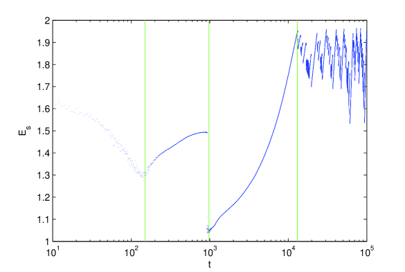
Figure 3: Temporal evolution of the threshold effort $E_{s}(t)$ for a system of $N=10000$ agents and imitation rate $r_{E}=0.04$. The initial form of the effort distribution is $f(E)=1$. The vertical lines help to distinguish the four different regimes.

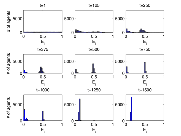
Figure 4: Histograms of the effort distribution $f(E)$ during the first two regimes. The initial $f(E)$ is uniform, $r_{E}=0.04$ and $N=10000$. The formation of the two peaks is followed by their competition leading to the disappearance of the peak in $E\approx\eta$.

1. Starting from any initial effort distribution $f(E)$, two narrow peaks are formed, one for $E\approx 0$ and the other at a value $\eta$ of the effort $E$.

2. The two peaks evolve and compete, until the peak in $\eta$ disappears.

3. The remaining peak drifts towards high values of $E$.

4. It eventually enters a sort of stationary state with intermittent oscillations about a large value of $E$.

This phenomenology occurs for any value of $r_{E}>0$, provided it is much smaller than 1, otherwise the system becomes completely random. The dependence on the initial shape of $f(E)$ is weak and does not change qualitatively the picture. We now describe in more detail the four regimes.

3.1 Initial regime: formation of two peaks

As intuitively expected from the static version of the model, agents will tend to imitate other agents with energies corresponding to the payoff maxima (see Fig. 2). This quickly leads to the collapse of the distribution function $f(E)$ in two peaks, one around 0 and the other around a finite value $\eta$ not far from the initial value of $E_{s}-1$ (see the first four panels of Fig. 4). At the same time, since the effort distribution varies, $E_{s}$ slowly changes in time (Fig. 3).

3.2 First intermediate regime: competition of the two peaks

When there are two peaks the dynamics can be monitored by two time-dependent quantities:

• $\eta(t)$: the average position of the second peak (the first is always around $E=0$).

• $\rho_{0}(t)$ the fraction of agents belonging to the first peak (obviously $\rho_{\eta}=1-\rho_{0}$).

Numerically, one observes that the peak in $\eta$ tends to move towards the right (and upward in Fig. 3), while simultaneously its total population decreases (i.e. $\rho_{0}$ grows). This is evident from Fig. 4, where the evolution of the effort distribution $f(E)$ is represented, and from Fig. 5, where $E_{s}$, $\rho_{0}$ and $\eta$ are reported as a function of time.

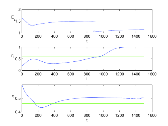
Figure 5: Behavior of the threshold energy $E_{s}$, the amplitude $\rho_{0}$ of the peak in $E=0$ and the position $\eta$ of the other peak, as a function of time in the first and second regime for a system with parameters $r_{E}=0.04$ and $N=10000$. The horizontal lines are for the values $\rho_{0}=7/12$ and $\eta=6/13$ (derived in the Appendix), that separate different regimes.

The drift of the second peak towards larger energies is easily understood qualitatively. The fundamental observation is that the threshold effort $E_{s}(t)$ falls within the peak in $\eta$, which has a width of the order of $\epsilon$. As a consequence, agents with energies in the left part of the peak will be less financed than those in the right part and then will tend to imitate them. The peak position slowly drifts towards right because of the struggle of agents to work just a little bit more than their colleagues.

The dynamics of $\rho_{0}(t)$ can be understood by making use of the simplifying assumption that the peaks are Dirac-$\delta$ functions. Under such assumption one can compute the expected payoff of agents in the two peaks as a function of $\rho_{0}$ and $\eta$ (Fig. 6). See the appendix for details about the derivation.

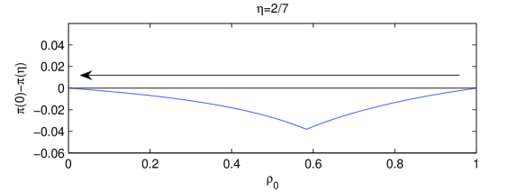
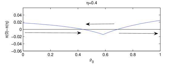
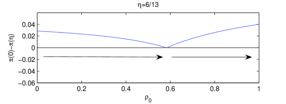
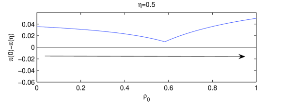
Figure 6: Behavior of the payoff difference $\pi(0)-\pi(\eta)$ between an agent with effort $E=0$ and one with effort $E=\eta$ as a function of $\rho_{0}$ for different values of $\eta$. The arrows indicate the direction of the dynamical evolution.

For small $\eta<2/7\approx 0.286\ldots$ the strategy $E=\eta$ is more convenient than $E=0$ for any value of $\rho_{0}$: agents in $\eta$ will be imitated and $\rho_{0}$ decreases.

For $2/7<\eta<6/13$ there are two values of $\rho_{0}$ for which the payoff of the two peaks is the same. The dynamics of $\rho_{0}(t)$ is much faster than the evolution of $\eta(t)$, as a detailed evaluation brings out that the rate of change ${\dot{\eta}}$ is smaller than ${\dot{\rho}}$ by a factor of the order of $\epsilon$. As a consequence, for any $\eta$, $\rho_{0}(t)$ assumes the stable “equilibrium” value corresponding to the leftmost point where the two payoffs are the same. The temporal evolution of $\rho_{0}(\eta)$ is then enslaved by the evolution of $\eta(t)$.

Finally, for $\eta>6/13$, the payoff of agents in zero is always larger than the payoff of agents in $\eta$. Therefore when this critical value is reached (corresponding to $\rho_{0}=7/12$) an abrupt change occurs: the threshold effort suddenly moves towards 1, the relative balance between the two peaks breaks down and rapidly the peak in $\eta$ disappears.

Notice that the passage from $E_{s}$ of the order $1+\eta$ to a value close to 1 is a rather intermittent process (Fig. 5): due to fluctuations associated with the random pairing of agents and the finiteness of $N$, for some time the threshold energy bounces back and forth between the two values before setting to a value close to 1.

3.3 Second intermediate regime: single peak drifting

Once a single peak is present, its position drifts towards larger effort values (Fig. 3) for reasons perfectly analoguous to what happened before to the peak in $\eta$: agents in the right part of the peak tend to be more successful and hence be imitated. In this “ideal” regime agents constantly improve themselves by devoting more and more effort to projects and less and less to the negotiation stage.

3.4 Asymptotic regime: strong intermittent oscillations

Also the ideal stage is doomed to end. This happens when the width of the peak $\Delta E^{*}$ becomes comparable to $1-E^{*}$, the distance from 1 of the peak position $E^{*}$. In such a case, a strategy in the extreme left tail of the peak becomes convenient, because the reduced chance of being financed is compensated by a strong advantage in the grant division. This leads to the formation of a secondary peak for $E\approx E^{*}-\Delta E^{*}$. At this point a competition between two peaks similar to the one of the First intermediate stage takes place, leading to a succession of cycles where the rightmost peak disappears, the remaining drifts towards 1 and then splits again in two peaks.

4 The role of mutations

We now consider the effect induced by the possibility of agents to mutate, i.e. to adopt a new strategy between $E=0$ and $E=1$ in a completely random way. The fraction of mutating agents per time step $r_{M}$ is taken to be much smaller than the imitation rate $r_{E}$, so that mutations do not completely change the general dynamics except for the possibility of agents to explore the whole space of strategies. In other words, they make the dynamics innovative, still preserving monotonicity with respect to the payoff rubinstein94 .

While the general picture remains the same, with the competition between two types of strategies, mutations modify the detailed phenomenology. In particular they make states with a single peak always unstable, thus preventing stages 3 and 4 of the mutationless case (second intermediate and asymptotic regimes) to be reached. After the initial formation of two peaks, the competition between them leads, as before, to growth of the peak in 0 and to the fast decay of the one in $\eta$. At this point it is necessary to distinguish between two possible cases.

If $r_{M}$ is extremely small with respect to $r_{E}$ (see below for details) mutated agents probe all possible effort values between $0$ and $\eta$ and one of them gives rise to a new peak that rapidly overcomes the others and starts drifting right. Once it goes beyond $\eta=2/7$, as it can be seen from Fig. 6, the strategy $E=0$ becomes again advantageous against agents in $\eta$ (with $\rho_{0}=0$). A peak in zero starts to grow, while $\eta$ grows further, bringing the system back to the first intermediate regime. The system enters therefore in a cycle with two peaks that cyclically collapse and reappear. (Fig. 7).

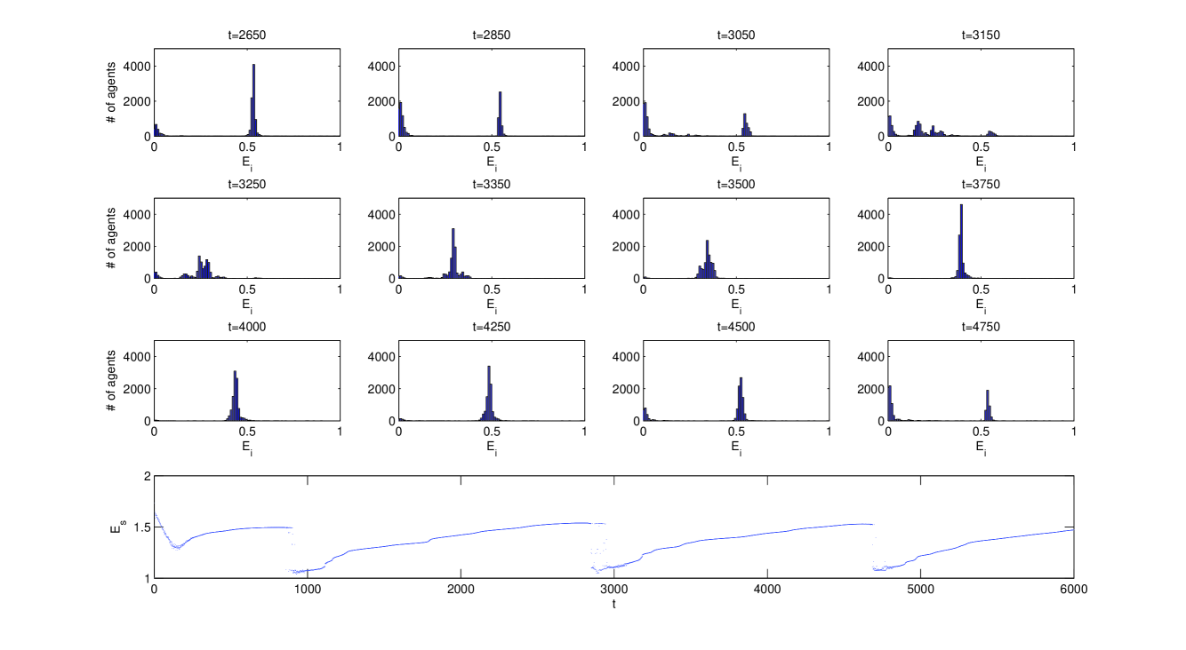
Figure 7: Temporal evolution of the histogram of the effort distribution $f(E)$ and of the threshold energy $E_{s}$ for a system with $r_{E}=0.04$, $N=10000$ and a very small mutation rate $r_{M}=0.0001$.

For larger values of $r_{M}$ (but still $r_{M}\ll r_{E}$) instead, the state with one peak in 0 and one in 0.5 becomes essentially evolutionary stable (Fig. 8). The populations of the two peaks will be around the critical values $\rho_{0}=7/12$, $\rho_{\eta}=5/12$. Depending on small variations of such populations, and on the creation of some agents with energies between them, $E_{s}$ will then fluctuate intermittently between $1$ to $1.5$

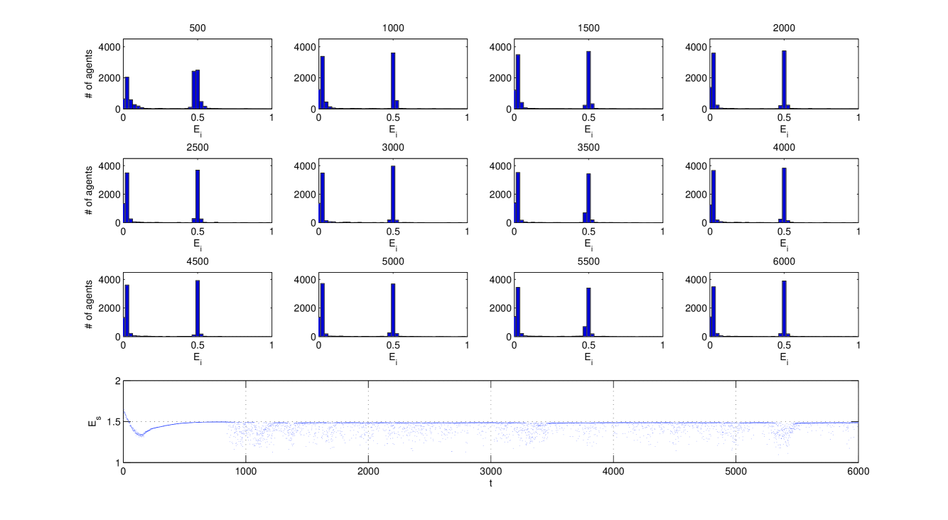
Figure 8: Temporal evolution of the histogram of the effort distribution $f(E)$ and of the threshold energy $E_{s}$ for a system with $r_{E}=0.04$, $N=10000$ and a small mutation rate $r_{M}=0.001$.

By considering different system sizes it turns out that the boundary between these two behaviors goes to a finite limit (of the order of $r_{M}/r_{E}\approx 10^{-2}$) when $N$ diverges.

5 Robustness of the phenomenology

What happens if some of the assumptions underlying the model are changed? In order to investigate the robustness of the phenomenology presented above, we consider several modifications applied to the model with both imperfect imitation and enough mutations to generate a stationary state with two peaks in equilibrium.

If the fraction of profits received by an agent, Eq. (1) is taken proportional to $(1-E)^{\alpha}$, with $\alpha>0$, simulations show that no qualitative change occurs with respect to the case $\alpha=1$, studied above.

Another possibility is to introduce some stochasticity in the probability to be approved. So far the probability for a project of total effort $E_{p}$ to be financed has a sharp threshold: $P(E_{p}>E_{s})=1$, $P(E_{p}<E_{s})=0$. If we consider instead a smooth function

$$P(E_{p})=\frac{1}{\exp\left[(E_{p}-E_{s})/T\right]+1},$$ (2)

it becomes possible that a project of relatively small value is financed while a better one (higher $E_{p}$) is not. Simulations again show that nothing changes qualitatively in the global behavior of the system, provided the “temperature” $T$ is not too high.

One parameter that turns out instead to affect noticeably the results is the fraction $Q$ of approved projects. So far we have always taken $P_{0}=P/2$, i.e. half of the projects were financed and half of them were not. For generic value of $Q=P_{0}/P$ projects can be distinguished in three categories. If both agents taking part to the project were not financed at the previous step then $E_{p}=2$. This occurs with probability $(1-Q)^{2}$. If one of them was financed (probability $2Q(1-Q)$) then $1\leq E_{p}\leq 2$; else, with probability $Q^{2}$, $0\leq E_{p}\leq 1$. After a transient stage, whose duration may vary with $Q$, the system settles in a stationary state. The properties of such state depend on the value of $Q$ leading to the identification of several different regimes, reflected in the behavior displayed in Fig. 9.

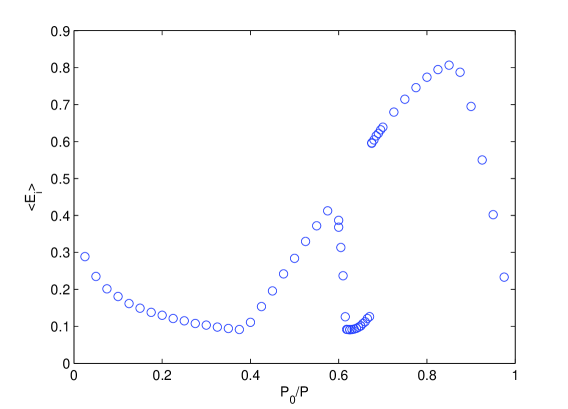
Figure 9: Average effort of agents in the stationary state as a function of $Q=P_{0}/P$. System parameters are $N=1000$, $r_{E}=0.04$, $r_{M}=0.005$.

For $Q\leq\frac{3-\sqrt{5}}{2}\approx 0.38$, since $(1-Q)^{2}>Q$ all financed projects have effort $E_{p}=2$, i.e. they involve partners that have not been financed at the previous step. The probability of being financed does not depend on $E$. Hence all agents converge to the $E=0$ strategy: too few financed projects push agents to laziness and greedy negotiations.

For $\frac{3-\sqrt{5}}{2}<Q<\frac{\sqrt{5}-1}{2}\approx 0.62$ the behavior is of the same type of the case studied so far $Q=1/2$, with the competition of two peaks, one in 0 and the other in $E=\eta$, whose amplitude goes to zero at the boundaries of the range.

For $Q>\frac{\sqrt{5}-1}{2}$ the situation is more involved. In general a single peak is formed rather than two. For $Q\approx 0.7$ the peak jumps from an effort close to zero to one larger than $1/2$, because the presence of agents with $E>1/2$ reinforces the profitability of such strategies.

It is important to remark that the presence of three distinct regions is related to the number of participants to each project $N_{p}=2$. For a generic $N_{p}$ there are $N_{p}+1$ zones, separated by points where the $E=0$ strategy dominates all others. Variations on $N_{p}$ have also other effects, mainly quantitative: the more partecipants per project, the less the agents tend to work. The second peak will move toward $0$. Of course when there are too many agents per project the two peaks eventually become indiscernible.

6 Conclusions

In this paper we have introduced a very simple model for the formation of collaborations in scientific projects and the ensuing stage where partners negotiate to share the awarded grants. The model includes only the main features of the process. It can therefore be viewed as describing a generic situation where agents have to collaborate within a group to compete globally for limited resources but also negotiate within the group to share the profit earned together.

In order to identify the most relevant effects and understand their role in the resulting phenomenology we have kept the description at a very basic level and perfomed an exploratory investigation, with no claim of considering any realistic situation. Despite these clear oversimplifications, the model displays some interesting, if not realistic, patterns of behavior.

Generically, within the two-stage game, the population of agents spontaneously clusters around two different strategies. “Hard workers” are characterized by relatively large values of the effort they put in the preparation of proposals. They tend to maximize the quality of their projects, so that a large fraction of them is financed. Consequently they put less effort in the negotiation stage. “Greedy” agents cluster instead around the strategy $E=0$, implying that they try to maximize their share when a grant is obtained. To do this they accept that their proposals are financed less frequently, and work hard only if this does not decrease their ability to argue about how to share the profits. Depending on the details of the model, the two populations are either in equilibrium or exhibit oscillations, but the existence of two classes of behavior is a robust feature.

Finally, the study of the dependence on the fraction of approved projects, shows that a small number of rejected projects is sufficient to push agents towards a state with minimum internal competition and large productive effort. On the other hand, when $Q$ is very small, so that the time lag between approved projects is large, agents tend to struggle for the scarce resources when they are available, instead of committing themselves to productive effort.

These interesting findings clearly call for additional investigations. In the spirit of going towards more realism, many possible variations of the model may be devised. One of the most natural is to consider heterogeneity either in agents’ intrinsic skills (the total effort available) or in the composition of projects (number of participants).

A further interesting direction has to do with extensions to interaction structures which are more constrained and realistic than the random matching assumed here. Preliminary results show, for agents placed on a square lattice, interesting spatio-temporal patterns with phase segregation between a population with $E\approx 0$ and $E\approx 1$, if both the ranges of imitation and collaboration are limited. A natural generalization of this has to do with allowing agents to select their neighbors depending on past performance. Preliminary results suggest that both constraining the interaction pattern and allowing agents to selectively choose neighbors generally increases the global performance of the system, as measured by the threshold effort $E_{s}$ for a project to be financed. The simultaneous evolution of the network of connections and of the distribution of agent strategies is another promising direction to follow. The systematic study of these effects deserves a systematic study to be discussed elsewhere.

Appendix

In this appendix we report the derivation of the payoff curves shown in Fig. 6. This is carried out assuming that each peak has vanishing width, so that it is mathematically described by a Dirac’s $\delta$ function. We take the first peak to be in $E=0$ and the second in $E=\eta$. In this case the system is fully described by the quantities $\rho_{0^{-}}$, the density of agents with zero effective effort, and $\eta$ that sets the effort of the other peak. The superscripts $+$ e $-$ represent agents that commit in the project an effective effort equal to $1$ or $E$, respectively.

At each time step the number of agents that does not receive a grant is half of the total. Hence $\rho_{+}=1/2$ and from the normalization condition $\rho_{0^{-}}+\rho_{\eta^{-}}+\rho_{+}=1$ one gets $\rho_{\eta^{-}}=\frac{1}{2}-\rho_{0^{-}}$.

The effort $E_{p}$ of a project, given by the sum of effective energies of two randomly selected agents, can be

• $0$, with probability $\rho_{0^{-}}^{2}$

• $\eta$, with probability $2\rho_{0^{-}}(\frac{1}{2}-\rho_{0^{-}})$

• $2\eta$, with probability $(\frac{1}{2}-\rho_{0^{-}})^{2}$

• $1$, with probability $2\frac{1}{2}\rho_{0^{-}}$

• $1+\eta$, with probability $2\frac{1}{2}(\frac{1}{2}-\rho_{0^{-}})$

• $2$, with probability $\frac{1}{4}$

Projects with total effort $E_{p}=2$ are always financed. Which of the other projects gets funded (and hence what is the threshold effort $E_{s}$) depends on the value of $\rho_{0}^{-}$ and $\eta$.

For $\rho_{0^{-}}\leq 1/4$ the projects with effort $E_{p}=1+\eta$ and $2$ are together more than half of the total number $P$. As a consequence $E_{s}$ will be $1+\eta$. Otherwise, if $\rho_{0^{-}}>1/4$, other projects are funded. For $\eta<1/2$, that is the relevant case, the remaining projects with higher effort are those with $E_{p}=1$, i.e. the projects with one partner in state + and one in state $0^{-}$.

The probability to be financed, as a function of the effective effort $E^{\rm eff}$ is then, for $\rho_{0^{-}}\leq 1/4$

$$P^{\#}(E^{\rm eff}=0) = 0$$ (3)

$$P^{\#}(E^{\rm eff}=\eta) = \frac{1}{4-8\rho_{0^{-}}}$$ (4)

$$P^{\#}(E^{\rm eff}=1) = \frac{3}{4}$$ (5)

In order to compute the expected payoffs one needs to evaluate, for agents with strategy $0$ ($\eta$) how many of them are in effective state $0^{+}$ ($\eta^{+}$) and how many in state $0^{-}$ ($\eta^{-}$). This is carried out by assuming that the populations in state $+$ or $-$ are in equilibrium, i.e. the rate of transition from $-$ to $+$ [$R(-\to+)$] is equal to the opposite rate $R(+\to-)$. This is reasonable because these processes are much quicker than all others, and in particular imitation. For the strategy $E=0$ this yields

$$R(-\to+) = \rho_{0^{-}}(1-P^{\#}(0^{-}))=\rho_{0^{-}}$$ (6)

$$R(+\to-) = \rho_{0^{+}}P^{\#}(+)=\frac{3}{4}\rho_{0^{+}},$$ (7)

so that

$$\rho_{0^{-}}=\frac{3}{7}\rho_{0}~{}~{}~{}~{}~{}~{}~{}~{}~{}~{}~{}~{}~{}~{}\rho_{0^{+}}=\frac{4}{7}\rho_{0}.$$ (8)

Similarly, for $E=\mu$

$$R(-\to+) = \rho_{\eta^{-}}\frac{3-8\rho_{0^{-}}}{4-8\rho_{0^{-}}}$$ (9)

$$R(+\to-) = \frac{3}{4}\rho_{\eta^{+}},$$ (10)

so that

$$\rho_{\eta^{-}}=\frac{3-6\rho_{0^{-}}}{6-14\rho_{0^{-}}}\rho_{\eta}~{}~{}~{}~{}~{}~{}~{}~{}~{}~{}~{}~{}~{}~{}\rho_{\eta^{+}}=\frac{3-8\rho_{0^{-}}}{6-14\rho_{0^{-}}}\rho_{\eta}.$$ (11)

From the condition on $\rho_{0^{-}}$ one obtains that $\rho_{0^{-}}\leq\frac{1}{4}$ if $\rho_{0}\leq\frac{7}{12}$.

We are now in the position to determine the average expected payoffs $\pi(0)$ and $\pi(\eta)$, by summing, over all possible pairings, the probability of such pairing times the associated expected payoff.

$$\pi(0) = \frac{21-8\eta\rho_{0}}{49(2-\eta)}$$ (12)

$$\pi(\eta) = \frac{98-84\rho_{0}+\eta(-49+32\rho_{0}^{2})}{196(2-\eta)(1-\rho_{0})}$$ (13)

The application of the same procedure with the appropriate values for $P^{\#}(E^{\rm eff})$ gives the expression of the average payoffs also for $\rho_{0^{-}}>1/4$ ($\rho_{0}>7/12$). The behavior of the payoff difference $\pi(\eta)-\pi(0)$ in the whole range of $\rho_{0}$ is plotted in Fig. 6.

Computation of $P^{\#}(E)$ for generic fixed $f(E)$ for the two stages game

When $f(E)$ is not a sum of $\delta$ functions, the computation is done in an iterative way. Considering $f(E)$ fixed (or slowly evolving, this can be done in a wide range of the parameters), we call $f_{t}(E)$ the varying effective distribution, changing in time because agents go to a $+$ or $-$ status. Starting from values at $t-1$, we compute values at $t$ in this way:

1. $f_{t}(E)=f(E)P^{\#}_{t-1}(E)+\frac{P_{0}}{P}\delta^{-}(E-1)$;

2. we convolve $f_{t}$ to obtain the probability density of the energy of the projects at time $t$, $f^{P}_{t}(E)=\int_{0}^{1}f_{t}(E^{\prime})f_{t}(E-E^{\prime})\mathrm{d}E^{\prime}$;

3. we obtain $E_{s}^{t}$ as the value such that $\int_{0}^{E_{s}^{t}}f^{P}_{t}\mathrm{d}E^{\prime}=\frac{P_{0}}{P}$;

4. at last, we compute $P^{\#}_{t}(E)=P^{\#}_{t-1}(E)\int^{1}_{Es-E}f_{t}(E^{\prime})\mathrm{d}E^{\prime})+(1-P^{\#}_{t-1}(E))\int^{1}_{Es-1}f_{t}(E^{\prime})\mathrm{d}E^{\prime}$.

This procedure allows to compute numerically $P^{\#}(E)$. A stable function, in very good agreement with simulations, is obtained after around 10 iterations. In Fig. 2 we used 80 iterations.

Once $P^{\#}(E)$ is found, it is easy to compute $\pi(E)$ considering all possible combinations of $+$ and $-$.

References

- (1) M. J. Osborne and A. Rubinstein, A course in Game Theory (MIT Press, Cambridge (MA), 1994)
- (2) R. Axelrod, W. D. Hamilton, Science 211 (1981) 1390-1396
- (3) W. Güth, R. Schmittberger, and B. Schwarze, Journal of Economic Behavior and Organization 3 (1982) 367-388
- (4) M. A. Nowak, K. M. Page and K. Sigmund, Science 289 (2000) 1773-1775
- (5) C. Castellano, S. Fortunato and V. Loreto, arXiv:0710.3256 (2007).
- (6) M. A. Nowak, Evolutionary Dynamics: Exploring the Equations of Life (Harvard University Press, Cambridge (MA), 2006)
- (7) M. A. Nowak, Science 314 (2006) 1560-1563
- (8) G. Szabó and G. Fáth, Phys. Rep. 446 (2007) 97-216
- (9) M. J. Barber, A. Krueger, T. Krueger and T. Roediger-Schluga, Phys. Rev. E 73 (2006) 036132
- (10) M. A. Nowak, J. theor. Biol. 142 (1990) 237-241
- (11) D. Cass, Journal of Economic Theory 4 200-223
- (12) A. Eriksson, K. Lindgren and T. Lundh, J. theor. Biol. 230 (2004) 319-332