The relation between star formation, morphology and local density in high redshift clusters and groups

Abstract

We investigate how the [OII] properties and the morphologies of galaxies in clusters and groups at $z=0.4-0.8$ depend on projected local galaxy density. We also compare our results with those derived from the field at similar redshifts and from clusters at low-z. In both nearby and distant clusters, higher-density regions contain proportionally fewer star-forming galaxies. At odds with low-z results, the relation between star-forming fraction and local density at high-z varies from high- to low-mass clusters, although is not solely a function of cluster mass. Both at high- and low-z, the average [OII] equivalent width (EW) of star-forming galaxies is independent of local density. However, in distant clusters the average current star formation rate in star-forming galaxies seems to peak at densities $\sim 15-40$ galaxies Mpc^-2. When using galaxy samples with similar mass distributions, we do not find large variations in the average EW(OII) and SFR properties of star-forming galaxies in the distant field, poor groups, and clusters. Overall, these results suggest that at high-z the current star formation activity in star-forming galaxies of a given galaxy mass does not depend strongly on global or local environment, though the possible SFR peak at intermediate densities seems at odds with this conclusion. We derive cluster-integrated star formation rates and find that the cluster SFR normalized by cluster mass anticorrelates with mass and correlates with the star-forming fraction, although we caution that the anticorrelation with mass could be mainly driven by correlated errors. We demonstrate that these trends can be understood given a) that the average star-forming galaxy forms about one solar mass per year (uncorrected for dust) in all our clusters; b) how the total number of galaxies scales with cluster mass; and c) the dependence of star-forming fraction on cluster mass. These findings show that the most fundamental open question currently remains why the evolution of the star-forming fraction depends on cluster mass. We present the morphology-density relation for our $z=0.4-0.8$ clusters, and uncover that the decline of the spiral fraction with density is entirely driven by galaxies of types Sc or later, while early spirals (Sa’s and Sb’s) have a flat distribution with density, similarly to that of S0s. For galaxies of a given Hubble type, we see no evidence that star formation properties (ongoing SFR, [OII] equivalent width, 4000 Å  break) depend on local environment. In contrast with recent findings at low-z, in our distant clusters the star formation-density relation and the morphology-density relation are equivalent, suggesting that neither of the two relations is more fundamental than the other. We suggest that the contrasting results at high- and low-z are partly due to different classification methods and/or to evolutionary effects giving rise to a progressive decoupling of the two relations at recent epochs.

1. Introduction

The star formation activity and other fundamental galaxy properties such as morphology and gas content vary systematically with redshift, galaxy mass and environment. While redshifts and galaxy masses are at least conceptually clearly defined, the definition of a galaxy environment is arbitrary and its optimal choice would require an a priori knowledge of the very thing we are trying to identify, that is the physical environmental driver or drivers of galaxy formation and evolution. Most studies nowadays define the “environment” either in terms of the local galaxy number density (the number of galaxies per unit volume or projected area around the galaxy of interest), or the virial mass of the cluster or group to which the galaxy belongs, when this applies, because these are the two most easily measurable quantities from spectroscopic or even imaging surveys.

In spite of environment being an elusive and arbitrary concept, the fact that galaxy properties depend on environment was recognized earlier than the dependence on galaxy mass and redshift (Hubble & Humason 1931). The first quantitative measurement of systematic differences with local environment was the so-called morphology-density relation (MDR) in nearby clusters. The MDR is the observed variation of the proportion of different Hubble types with local density, with ellipticals being more common in high-density regions, spirals being more common in low-density regions, and S0s making up a constant fraction of the total population within the cluster virial radius regardless of density (Dressler 1980, as revisited in Dressler et al. 1997). It was subsequently found that a similar MDR also exists in nearby groups (Postman & Geller 1984 also revisited in Postman et al. 2005) and that a qualitatively similar, but quantitatively different, MDR is present in galaxy clusters at redshifts up to 1 (Dressler et al. 1997, Treu et al. 2003, Smith et al. 2005, Postman et al. 2005).

Galaxy stellar populations have also long been known to vary systematically with environment (Spitzer & Baade 1951): denser environments have on average older stellar populations. At least at some level, this must be related to the higher incidence of early-type galaxies in high density regions, i.e. to the morphology-density relation. At low redshift the best characterization of the “star formation-local density” (SFD) relation has come from large redshift surveys. These studies have conclusively demonstrated that the average galaxy properties related to star formation depend on local density even at large clustercentric radii; at low densities in clusters; and outside of clusters, in groups and the general field (Hashimoto et al. 1998, Lewis et al. 2002, Gomez et al. 2003, Kauffmann et al. 2004, Balogh et al. 2004, see also Pimbblet et al. 2002). Moreover, they have highlighted the dependence on both galaxy mass and local environment, showing strong environmental trends at a given galaxy mass (Kauffmann et al. 2004, Baldry et al. 2006).

To understand the origin of the SFD relation, it is essential to answer two separate questions: at any given galaxy mass, 1) how does the proportion of star-forming galaxies vary with density, and 2) how does the star formation activity in star-forming galaxies vary with density? At low-z, the evidence for a change in the relative numbers of red/passively-evolving and blue/star-forming galaxies with local environment is overwhelming, but it remains an open question whether star-forming galaxies of similar mass have star formation histories that depend on local density (Balogh et al. 2004a,b, Hogg et al. 2004, Gomez et al. 2003, Baldry et al. 2006).

Deep redshift surveys have recently extended the study of the SFD relation in the general field to high redshift. They have revealed that the number ratio of red to blue galaxies increases with local density out to $z>1$ and that we might be witnessing the establishment of the color-density relation at $z$ approaching 1.5 (Cucciati et al. 2006, Cooper et al. 2007, Cassata et al. 2007). This suggests that the transition from a star-forming phase to a passive one occurs for a large number of massive galaxies in groups at $z\sim 2$ (Poggianti et al. 2006). In apparent but not substantial contradiction, the average SFR per galaxy at $z=1$ increases instead of decreasing with local density. Therefore the SFD relation is inverted with respect to the local Universe (Elbaz et al. 2007, Cooper et al. 2008).

Thus, the MDR up to $z=1$ is well studied in clusters and has started to be explored in the field (Capak et al. 2007), and the SFD relation is now being investigated in the general field over a similar redshift baseline. In clusters, Moran et al. (2005) have presented the EW(OII)s of ellipticals and S0 galaxies as a function of local density for a cluster at $z=0.4$. However, a detailed study of the relation between star-formation and local environment in distant clusters has not yet been carried out. As a consequence, a comparison of the MDR and the SFD relation has not been possible to date in clusters at high redshift. This is due to the limited number of well-studied distant clusters with homogeneous data.

Deep galaxy redshift surveys have recently made it possible to characterize the global as well as the local environment of galaxies and to study significant samples of groups at high-z (Wilman et al. 2005, Gerke et al. 2005, Balogh et al. 2007, Gerke et al. 2007, Finoguenov et al. 2007). Groups are typically identified as galaxy associations with masses $<10^{14}\,M_{\odot}$ corresponding to velocity dispersions of $\lesssim 400\,\rm km\,s^{-1}$. Even the largest field surveys, however, include only very few distant systems above this mass (Finoguenov et al. 2007, Gerke et al. 2007). On the other hand, until recently, distant cluster surveys have studied primarily massive clusters. Only the latest surveys of optically-selected samples target structures of a wide range of masses, down to the group level (Hicks et al. 2008, Gilbank et al. 2008, Milvang-Jensen et al. 2008, Halliday et al. 2004). Nowadays groups are therefore the meeting point of field and cluster studies at high-z, and it has become possible to study the dependence of the SFD relation on global environment (clusters, groups and the field), approaching the question from both perspectives.

In this paper, we investigate the relation between star formation activity, morphology and local galaxy density in $z=0.4-0.8$ clusters and groups observed by the ESO Distant Cluster Survey (EDisCS). The EDisCS data set permits an internal comparison with galaxies in poor groups and the field at the same redshifts in a homogeneous way. To compare our results with clusters in the nearby Universe, we use a cluster sample drawn from the Sloan Digital Sky Survey (SDSS).

After presenting the data set (§2) and the definition of our cluster, group and field samples (§3), we outline our method for measuring the local galaxy density at high-z (§4) and describe the low-z cluster sample we use as local comparison (§5). The average trends of the fraction of star-forming galaxies and of the [OII] equivalent width with local density in clusters (§6.1) is compared with those found in lower density environments in §6.2 and to those in low-z clusters in §6.4. The dependence of the star-forming fraction on global cluster properties is presented in §6.3. We then analyze the behavior of the average and specific star formation rates in §7, summarizing the similarities and differences of the EW-density and SFR-density relations in §7.1. Cluster-integrated star formation rates are derived in §7.2 where we show their relationship with cluster mass and other global cluster properties. Galaxy morphologies are discussed in §8, where we present the morphology-density relation, the star-forming properties of each Hubble type as a function of local density, and the link between the MD and the SFD relations. The latter is compared with results at low redshift in §8.1. Finally, we summarize our conclusions in §9.

All equivalent widths and cluster velocity dispersions are given in the rest frame. All quantities related to star formation are given uncorrected for dust. We use proper (not comoving) radii, areas and volumes. We assume a $\Lambda$CDM cosmology with ($H_{0}$, ${\Omega}_{m}$, ${\Omega}_{\lambda}$) = (70,0.3,0.7).

2. The dataset

The ESO Distant Cluster Survey (hereafter, EDisCS) is a multiwavelength survey of galaxies in 20 fields containing galaxy clusters at $z=0.4-1$.

Candidate clusters were selected as surface brightness peaks in smoothed images taken with a very wide optical filter ($\sim$ 4500-7500 Å) as part of the Las Campanas Distant Cluster Survey (LCDCS; Gonzales et al. 2001). The 20 EDisCS fields were chosen among the 30 highest surface brightness candidates in the LCDCS, after confirmation of the presence of an apparent cluster and of a possible red sequence with VLT 20 min exposures in two filters (White et al. 2005).

For all 20 fields EDisCS has obtained deep optical photometry with FORS2/VLT, near-IR photometry with SOFI/NTT, multislit spectroscopy with FORS2/VLT, and MPG/ESO 2.2/WFI wide field imaging in $VRI$. ACS/HST mosaic imaging in $F814W$ of 10 of the highest redshift clusters has also been acquired (Desai et al. 2007). Other follow-up programmes include XMM-Newton X-Ray observations (Johnson et al. 2006), Spitzer IRAC and MIPS imaging (Finn et al. in prep.), $\rm H\alpha$ narrow-band imaging (Finn et al. 2005), and additional optical imaging and spectroscopy in 10 of the EDisCS fields targeting galaxies at $z\sim 5$ (Douglas et al. 2007).

An overview of the survey goals and strategy is given by White et al. (2005), who also present the optical ground–based photometry. This consists of $V$, $R$ and $I$ imaging for the 10 highest redshift cluster candidates, aimed at providing a sample at $z\sim 0.8$ (hereafter the high-z sample) and $B$, $V$ and $I$ imaging for 10 intermediate–redshift candidates, aimed to provide a sample at $z\sim 0.5$ (hereafter the mid-z sample). In practice, the redshift distributions of the high-z and the mid-z samples partly overlap (Milvang-Jensen et al. 2008).

Spectra of $>100$ galaxies per cluster field were obtained, with typical exposure times of 4 hours for the high-z sample and 2 hrs for the mid-z sample. Spectroscopic targets were selected from I-band catalogs (Halliday et al. 2004). At the redshifts of our clusters, this corresponds to $\sim 5000\pm 500$ Å  rest frame. Conservative rejection criteria based on photometric redshifts (Pelló et al. in prep.) were used in the selection of spectroscopic targets to reject a significant fraction of non–members while retaining a spectroscopic sample of cluster galaxies equivalent to a purely I-band selected one. A posteriori, we verified that these criteria have excluded at most 1-3% of cluster galaxies (Halliday et al. 2004 and Milvang-Jensen et al. 2008). The spectroscopic selection, observations, and catalogs are presented in Halliday et al. (2004) and Milvang-Jensen et al. (2008).

In this paper we make use of the spectroscopic completeness weights derived by Poggianti et al. (2006). Here we only give a brief summary of the completeness of our spectroscopic sample, referring the reader to the previous paper for details. Given the long exposure times, the success rate of our spectroscopy (number of redshift/number of spectra taken) is 97% above the magnitude limit used in this study. A visual inspection of the remaining 3% of the galaxies reveals that most of these are bright, featureless low-z galaxies. Moreover, in our previous paper we computed the spectroscopic completeness as a function of galaxy magnitude and position within the cluster (Appendix A), verified the absence of biases in the completeness-corrected sample (Appendix B) and found that incompleteness has a negligible effect on the [OII] properties of our clusters.

In this paper, we analyze 16 of the 20 fields that comprise the original EDisCS sample. We exclude two fields that lack several masks of deep spectroscopy (cl1122.9-1136 and cl1238.5.114; see Halliday et al. 2004 and White et al. 2005). We also exclude two additional systems (cl1037.9-1243 and cl1103.7-1245), each of which has a neighboring rich structure at a slightly different redshift (Milvang-Jensen et al. 2008) that is indistinguishable on the basis of photometric properties alone. The names, redshifts, velocity dispersions, and numbers of spectroscopic members for the remaining 16 clusters are listed in Table 1.

The EDisCS spectra have a dispersion of 1.32 Å/pixel or 1.66 Å/pixel, depending on the observing run. They have a FWHM resolution of $\sim 6$ Å, corresponding to rest-frame 3.3 Å  at z=0.8 and 4.3 Å  at z=0.4. The equivalent widths of [Oii] were measured from the spectra using a line-fitting technique, as outlined in Poggianti et al. (2006). This method includes visual inspection of each 1D spectrum. Each line detected in a given 1D spectrum was confirmed by visual inspection of the corresponding 2D spectrum; this is especially useful to assess the reality of weak [Oii] lines.

We do not attempt to separate a possible AGN contribution to the [OII] line, or to exclude galaxies hosting an AGN. We are unable to identify AGNs in our data, as the traditional optical diagnostics are based on emission lines that are not included in the spectral range covered by most of our spectra.

AGN contamination will be most relevant for our study if there are non-starforming, red galaxies in which the [OII] emission originates exclusively from processes other than star formation. We note that only 13% of the spectroscopic sample used here is composed of red galaxies with a detected [OII] line in emission. About 40% of these are spirals of types Sa or later. Among local field galaxies, about half of the red [OII]-emitting galaxies are LINERs whose source of ionization is still debated, while the rest are either star-forming or Seyferts/transition objects in which star formation dominates the line emission (Yan et al. 2006). Adopting the distribution of AGN types observed locally in the field and conservatively assuming that all LINERs are devoid of star formation, we estimate that the contamination from pure AGNs in our sample is at most 7%. Moreover, we have verified that the fraction of red emission-line galaxies is not a function of local density. It remains true, however, that all the trends we observe, and their evolution, may reflect a combination of the variations in the level of both star formation activity and AGN activity. This should be kept in mind throughout the paper and when comparing our results with any other work.

With these caveats in mind, we conveniently refer to galaxies interchangeably as “star-forming” or “[Oii] galaxies” whenever their EW([Oii] )$>3$ Å , adopting the convention that EWs are positive in emission. The detection of the [OII] line above this EW limit is essentially complete in our spectroscopic sample (see Poggianti et al. 2006 for details).

Table 1List of clusters.

Cluster name	Short name	$z$	$\sigma$ $\pm{\delta}_{\sigma}$	$N_{mem}$
			$\rm km\,s^{-1}$
Cl 1232.5-1250	Cl 1232	0.5414	1080 ${}_{-89}^{+119}$	54
Cl 1216.8-1201	Cl 1216	0.7943	1018 ${}_{-77}^{+73}$	67
Cl 1138.2-1133	Cl 1138	0.4798	732 ${}_{-76}^{+72}$	49
Cl 1411.1-1148	Cl 1411	0.5201	710 ${}_{-133}^{+125}$	22
Cl 1301.7-1139	Cl 1301	0.4828	687 ${}_{-86}^{+81}$	35
Cl 1353.0-1137	Cl 1353	0.5883	666 ${}_{-139}^{+136}$	20
Cl 1354.2-1230	Cl 1354	0.7627	648 ${}_{-110}^{+105}$	21
Cl 1054.4-1146	Cl 1054-11	0.6972	589 ${}_{-70}^{+78}$	49
Cl 1227.9-1138	Cl 1227	0.6355	574 ${}_{-75}^{+72}$	22
Cl 1202.7-1224	Cl 1202	0.4244	518 ${}_{-104}^{+92}$	19
Cl 1059.2-1253	Cl 1059	0.4561	510 ${}_{-56}^{+52}$	41
Cl 1054.7-1245	Cl 1054-12	0.7498	504 ${}_{-65}^{+113}$	36
Cl 1018.8-1211	Cl 1018	0.4732	486 ${}_{-63}^{+59}$	33
Cl 1040.7-1155	Cl 1040	0.7043	418 ${}_{-46}^{+55}$	30
Cl 1420.3-1236	Cl 1420	0.4959	218 ${}_{-50}^{+43}$	24
Cl 1119.3-1129	Cl 1119	0.5500	166 ${}_{-29}^{+27}$	17

3. The definition of the various environments

As can be seen in Table 1, EDisCS structures cover a wide range of velocity dispersions, from massive clusters to groups. For brevity, we will refer collectively to these structures as “EDisCS clusters”. In addition, within the EDisCS data set it is possible to investigate the spectroscopic properties of galaxies in even less densely populated environments, at the same redshift as our main structures.

In a redshift slice within $\pm 0.1$ in $z$ from the cluster/group targeted in each field, where we are sure the spectroscopic catalog can be treated as a purely I-band selected sample with no selection bias, we have identified other structures as associations in redshift space as described in Poggianti et al. (2006) . These associations have between 3 and 6 galaxies and will hereafter be referred to as “poor groups”. We did not attempt to derive velocity dispersions for these systems, given the small number of redshifts per group. In total, our poor group sample comprises 84 galaxies brighter than the magnitude limits adopted for our analysis (absolute V magnitude brighter than -20, see below).

Finally, within the same redshift slices, any galaxy in the spectroscopic catalogs that is not a member of our clusters, groups or poor group associations is treated as a “field” galaxy. This field galaxy sample is composed of 162 galaxies brighter than our limit and should be dominated by galaxies in regions less populated and less dense than the clusters and groups, although will also contain galaxies belonging to poor structures that went undetected in our spectroscopic catalog. Our field sample is therefore far from being similar to the galaxy sample in general “field” studies, which will be dominated by a combination of group, poor group, and field galaxies according to our environment definition.

The median redshift is 0.58 for the field sample and 0.66 for the poor group sample. Redshift and EW([OII]) distributions of our poor group and field samples are given in Poggianti et al. (2006) . Computing galaxy masses as outlined in §7, we find that the mass distribution of galaxies varies significantly with environment, progressively shifting towards higher masses from the field to the poor groups to the clusters. This corresponds to a difference in the galaxy luminosity distributions, which was shown in Poggianti et al. (2006) . We build field and poor group samples that are matched in mass to the cluster sample (hereafter the “mass-matched” field and poor group samples), drawing for each cluster galaxy a field or poor group galaxy with a similar mass. In the following, we will present the results for both mass-matched and unmatched samples, but show only mass-matched values in all figures.

4. Projected local galaxy densities

The projected local galaxy density is computed for each spectroscopically confirmed member of an EDisCS cluster. It is derived from the circular area $A$ that in projection on the sky encloses the N closest galaxies brighter than an absolute V magnitude $M_{lim}^{V}$. The projected density is then $\Sigma$ = N/$A$ in number of galaxies per square megaparsec. In the following we use N=10, as have most previous studies at these redshifts. For about 7% of the galaxies in our sample, the circular region containing the 10 nearest neighbors extends off the chip. Since the local densities of these sources suffer from edge effects, they were excluded from our analysis.

Densities are computed both by adopting a fixed magnitude limit $M_{lim}^{V}=-20$ and by letting $M_{lim}^{V}$ vary with redshift between -20.5 at $z=0.8$ and -20.1 at $z=0.4$ to account for passive evolution. Absolute galaxy magnitudes are derived as described in Poggianti et al. (2006) . We have used two different radial limits to derive the mean properties of galaxies in each density bin. First, we tried using only galaxies within $R_{200}$ (the radius delimiting a sphere with an interior mean density of 200 times the critical density, approximately equal to the cluster virial radius). We also tried including all galaxies in our spectroscopic sample, regardless of distance from the cluster center. The values of $R_{200}$ computed for our clusters, as well as sky maps showing $R_{200}$ relative to the extent of the spectroscopic sample, are given in Poggianti et al. (2006). For most clusters, our spectroscopy extends to $R_{200}$, while severe incomplete radial sampling occurs for one cluster, Cl1232, which will be treated separately when relevant, e.g. in §7.2. The results do not change whether we confine our analysis to $R_{200}$ or use our full spectroscopic sample, nor whether we use a fixed or a varying magnitude limit. Therefore, to maximise the number of galaxies we can use and to minimize the statistical errors, we show the results for $M_{lim}^{V}=-20$ and with no radial limit, unless otherwise stated.

We apply three different methods to identify the 10 cluster members that are closest to each galaxy. These yield three different estimates of the projected local density, which we compare in order to assess the robustness of our results.

In the first method, the density is calculated using all galaxies in our photometric catalogs and is then corrected using a statistical background subtraction. The number of field galaxies within the circular area $A$ and down to the magnitude limit adopted for the cluster is estimated from the $I$-band number counts derived for a 4 deg x 4 deg area by Postman et al. (1998).

In the other two methods we include only those galaxies that are considered cluster members according to photometric redshift estimates. As described in detail in Pelló et al. (in prep.), photometric redshifts were computed for EDisCS galaxies using two independent codes: a modified version of the publicly available Hyperz code (Bolzonella, Miralles & Pelló 2000), and the code of Rudnick et al. (2001) with the modifications presented in Rudnick et al. (2003). We use two different criteria to retain cluster members and reject probable non-members. In the first case, a galaxy is accepted as a cluster member if the integrated probability that the galaxy lies within $\pm 0.1$ in $z$ from the cluster redshift is greater than a specific threshold for both photometric redshift codes. The probability threshold is chosen to retain about 90% of the spectroscopically confirmed members in each cluster. In the other method a galaxy is retained as a cluster member if the best photometric estimate of its redshift from the Hyperz code is within $\pm 0.1$ in $z$ from the cluster redshift. The projected local density distributions obtained with the three methods are shown in Fig. 1.

We note that throughout the paper we use only proper (not comoving) lengths, areas, and volumes. For example, our local densities are given as the number of galaxies per $\rm Mpc^{2}$, as measured by the rest-frame observer. This choice is dictated by the fact that with local densities we are investigating vicinity effects, and gravitation depends on proper distances.

5. Low redshift sample

Using the SDSS, we have compiled a sample of clusters and groups at $0.04<z<0.1$. This sample serves as a low-redshift baseline with which we can compare our high-z results. The SDSS cluster sample is described in Poggianti et al. (2006) and comprises 23 Abell clusters with velocity dispersions between 1150 and 200 $\rm km\,s^{-1}$, with an average of 35 spectroscopically confirmed members per cluster. To approximate the EDisCS spectroscopic target selection, which was carried out at rest-frame $5000\pm 500$ Å , we used a $g$-selected sample extracted from the SDSS spectroscopic catalogs.

Local densities were computed for spectroscopic cluster members (within 3$\sigma$ from the cluster redshift) that lie within $R_{200}$ from the cluster center. For Sloan, the radial cut is necessary to approximate the EDisCS areal coverage, which reaches out to about $R_{200}$. We choose a galaxy magnitude limit of $M_{V}<-19.8$, which maximizes the number of galaxies we can use in our analysis and would correspond to $-20.1$ at $z=0.4$ and $-20.5$ at $z=0.8$ under the assumption of passive evolution.

As for EDisCS, local densities were derived using the circular area encompassing the 10 nearest neighbors. Two methods were employed to obtain two independent estimates of local densities. In the first method, we find the distance to the tenth-nearest projected neighbor considering only spectroscopically confirmed members brighter than $M_{V}<-19.8$. In the second method, we include the 10 nearest projected neighbors that are within the Sloan photometric catalog and that have an estimated absolute magnitude satisfying $M_{V}<-19.8$. Absolute magnitudes were derived from observed magnitudes assuming that all galaxies lie at the cluster redshift and using the transformations of Blanton et al. (2003). Both the spectroscopic and the photometric densities were computed from catalogs of galaxies located over an area much larger than $R_{200}$ to avoid edge effects.

Since the spectroscopic completeness within $R_{200}$ of the SDSS clusters is on average about 84%, the first method is likely to underestimate the “true” density. Using only the photometric catalog, we ignore the fact that some of the 10 galaxies might be in the background or foreground of the cluster. The second method therefore overestimates the value of the density. Thus, the spectroscopically-based and photometrically-based local densities represent lower and upper limits to the local density. Density values that have been corrected for spectroscopic incompleteness and for background contamination will lie between these two values.

The local density distributions derived with the two methods are shown in the right panel of Fig. 1. As expected, the distribution of spectroscopically-based densities is shifted to slightly lower densities than the distribution based on photometry, but in the following we will see that the conclusions reached by the two methods are fully consistent. Compared to the density distribution at high-z shown in the left panel of the same figure, the low-z distribution is shifted to lower densities. In Poggianti et al. (in prep.) we show this is due to the fact that high-z clusters are on average denser by a factor of $(1+z)^{3}$ compared to nearby clusters, with possible strong consequences on galaxy evolution.

The values of EW([Oii] ) measured with the method we used for EDisCS spectra are in very good agreement with those measured by Brinchmann et al. (2004a,b) for star-forming galaxies in the SDSS (see Fig. 3 in Poggianti et al. (2006)). However, for EDisCS galaxies, the EW([Oii] ) was measured only when the line was present in emission, and a value EW([Oii] )=0 was assigned when no line was present. In addition, each 1D and 2D spectrum was visually inspected. In contrast, the SDSS [Oii] measurements of Brinchmann et al. (2004a,b) are fully automated and can even yield a (small) value in absorption that is compatible with 0 within the error and that cannot be ascribed to the [Oii] 3727 line. To take this into account, for SDSS clusters we have used the EWs provided by Brinchmann et al. (2004a,b), but have forced the EW([Oii] ) to be equal to 0 when the value provided by Brinchmann et al. is $EW<0.8$ Å  in emission. Moreover, to be compatible with EDisCS, we do not exclude AGNs from our SDSS analysis. Finally, the redshift range of our Sloan clusters was chosen as a compromise to minimize aperture effects while still sampling sufficiently deep into the galaxy luminosity function. The $3\arcsec$ SDSS fiber diameter covers the central 2.4-5.4 kpc of galaxies depending on redshift, compared to the $1\arcsec$ EDisCS slit covering 5.4-7.5 kpc at high redshift. In the following, we assume that [OII] equivalent widths do not change significantly over these different areas.

6. Results

6.1. [Oii] strength and star-forming fractions as a function of local density at high-z

We first investigate how the strength of the [Oii] line varies in EDisCS clusters as a function of projected local density. Figure 2 shows the mean equivalent width of [Oii] measured over all galaxies that are spectroscopically confirmed members of EDisCS clusters (black symbols), in bins of local density. The three different estimates of density described in §3 (empty and filled circles and crosses) yield similar results within the errors. In the following, errors on mean equivalent widths are computed as bootstrap standard deviations, and errors on fractions are computed from Poissonian statistics.

The mean EW computed over all galaxies is consistent with being flat up to a density $\sim 70\,\rm gal/Mpc^{2}$ (the Kendall’s probability for an anticorrelation in the three lowest density bins is only 40%), then decreases at higher densities. These trends arise from a combination of the incidence of star-forming galaxies and the relation between density and EW in star-forming galaxies.

As shown in fig. 3, the proportion of star-forming galaxies tends to decline at higher density. The fraction of star-forming galaxies decreases from about 60% to $\leq$30%. Using the average of the values given by the 3 membership methods, the Kendall test gives a 95% probability of an anticorrelation.

In contrast, fig. 4 shows that the mean EW([Oii] ) computed only for galaxies with emission lines does not correlate with local density (the Kendall’s correlation probability is 38%). It is consistent with being flat over most of the density range, except for the highest density bin centered on $\sim 450$ galaxies per $\rm Mpc^{2}$, where it drops by a factor 2 to 3. As will be shown in §8, the highest density bin is populated only by elliptical galaxies, whose weak [OII] may be related to the presence of an AGN. It is thus not surprising that this bin stands out from the other bins, where star-forming spirals dominate the mean behavior.

The constancy of the average [Oii] equivalent width in star-forming galaxies at most densities suggests that as long as star formation is active, it is on average unaffected by local environment, at least in clusters.

6.2. Comparison with poor groups and the field at $z=0.4-0.8$

The mean EW([Oii] ) among all of our field galaxies is 10.7$\pm$1.5 Å  for the mass-matched sample (dashed lines in fig. 2), and 13.5$\pm$1.5 Å  for the unmatched sample. Similar values are found for poor group galaxies: 11.6$\pm$1.8 Å  for the mass-matched sample (dotted lines) and 14.5$\pm$1.8 Å  for the unmatched sample. These values are comparable within the uncertainties to the values measured in the low density regions of the clusters.

Similarly, when considering only galaxies with ongoing star formation, the mass-matched field and poor group values are comparable to those at most densities in clusters (fig. 4). The mean EW of [Oii] field and poor group galaxies is 17.2$\pm$1.5 Å  and 14.5$\pm$2.2 Å , respectively (18.0$\pm$1.5Å  and 18.9$\pm$2.2Å  in the unmatched samples).

Finally, the fraction of [Oii] galaxies in the field is 62$\pm 8$% (matched, fig. 3) and 72$\pm 8$% (unmatched). In the poor groups, the mass-matched [Oii] fraction is 80.0 $\pm 10$% (matched) and 77$\pm 10$% (unmatched). The star-forming fraction in the field is compatible with that observed at most densities in clusters, while the poor group fraction is slightly higher.

Therefore, relative to clusters, the unmatched poor groups and field have higher average EWs and star-forming fractions. Our results indicate that this is primarily due to differences in the galaxy mass distribution with environment. Using galaxy samples with similar mass distributions, we find that the EW properties of star-forming galaxies do not differ significantly between clusters, poor groups, and the field, neither with local density within clusters as shown in the previous section.

6.3. [Oii] -local density relation as a function of cluster mass

To assess whether the relation between star formation and density is the same in structures of different mass, we divide our cluster sample into different velocity dispersion bins and show the correlation found above, between the star-forming fraction and density, in Fig.5. The analysis is now done using only galaxies within $R_{200}$. As above, errors on fractions are computed from Poissonian statistics.

The two most massive clusters ($\sigma>800\,\rm km\,s^{-1}$ ) exhibit a flatter relation. i.e. have lower [OII] fractions in the three lowest density bins, than clusters with $\sigma<800\,\rm km\,s^{-1}$.

In contrast, we find that at low-z this relation is indistinguishable in clusters with $\sigma$ above and below $800\,\rm km\,s^{-1}$, in agreement with previous works that found no dependence of the correlation between the star-forming ($\rm H\alpha$-emitting) fraction and density from the cluster velocity dispersion in the local universe (Lewis et al. 2002, Balogh et al. 2004).

We note that although the relation between [OII] fraction and local density varies with cluster mass at high-z, the relation between star formation and physical three-dimensional space density may be constant, since the distribution of physical densities in each projected 2D density bin varies with cluster mass (Poggianti et al. in prep.).

Dividing the high-z sample into finer velocity dispersion bins, we do not find a continuous trend with velocity dispersion (Fig.5). Systems with $600<\sigma<800\,\rm km\,s^{-1}$ may lie at larger or comparable [OII] fractions than systems with $\sigma<600\,\rm km\,s^{-1}$, but our errorbars are too large to draw any conclusion.

In Poggianti et al. (2006) we studied how the fraction of [OII] galaxies depends on the cluster velocity dispersion $\sigma$. In an [OII] fraction-$\sigma$ diagram, one can identify three groups of structures: a) high-mass structures, all with low [OII] fractions; b) low-mass structures with high [OII] fractions and c) low-mass structures with low [OII] fractions (the so-called “outliers” in Poggianti et al. (2006) ). In addition to having a low [OII] fraction, the outliers have a low fraction of blue galaxies (De Lucia et al. 2007), a high fraction of early-type galaxies given the measured velocity dispersions (Simard et al. 2008), and peculiar [OII] equivalent width distributions (Poggianti et al. (2006) ). Hence, galaxies in the outliers resemble those in the cores of much more massive clusters.

The presence of low-mass structures with low [OII] fractions in our sample could be responsible for a non-monotonic trend of the [OII] fraction-density relation with cluster mass. We study the dependence of the [OII] fraction on local projected density for the three groups separately in the right panel of Fig.5.

Except for the lowest density bin where the results of all three groups are compatible within the errors, the trend with local density is different in the three groups. At any given density, the star-forming fraction in low-mass, low-[OII] groups is significantly lower than those in low-mass high-[OII] systems.

In Poggianti et al. (2006) we found that the global [OII] fraction in distant clusters relates to the system mass, but not solely to the system mass, at least as estimated from the observed velocity dispersion. Here we find that the [OII] fraction does not depend solely on projected local density but also on global environment, and that variations in the star-forming fraction-density relation do not depend uniquely on cluster mass. In principle, the correlations with system mass and local density could have a single common origin, from i.e. a correlation between galaxy properties and physical density in three-dimensional space. In a separate paper (Poggianti et al. in prep.), we use numerical simulations to investigate the relations between projected local density, physical 3D density, and cluster mass. The aim of that paper is a simultaneous interpretation of the observed trends with local density and cluster mass presented in this paper and in Poggianti et al. (2006) .

6.4. The EW([OII])-density relation at low redshift

The SDSS results are shown as red symbols (triangles) in fig. 2, fig. 3 and fig. 4. At low-z, the mean EW([Oii] ) computed for all galaxies continuously and smoothly decreases with local density (fig. 2). This trend is driven by the decrease in the star-forming fraction with local density (fig. 3). Using the average of the values obtained with the two density estimates, the Kendall’s test yields a 98.5% probability of an anti-correlation.

As at high-z, the mean [Oii] strength of [Oii] -galaxies does not vary significantly over most of the density range (Kendall’s probability 82.6%), except for a decrease in the highest density bin (fig. 4). These findings are in agreement with previous low-z results based on SDSS and 2dFGRS (Lewis et al. 2002, Balogh et al. 2004).

From a quantitative point of view, blindly comparing the high-z and the low-z results, at any projected density in common we observe a lower average EW([OII]) at low-z. This is due to both a lower average [OII] fraction and a lower average EW([OII]) in star-forming galaxies at low-z. Taken at face value, this indicates that both the proportion of star-forming galaxies and the star formation activity in them decrease with time at a given density. However, it is worth stressing that observing similar projected densities at different redshifts does not imply similar physical densities, since the correlation between projected and 3D density varies with redshift (Poggianti et al. in prep.). Hence, a quantitative comparison of results at different epochs at a given projected density cannot be interpreted as a direct measure of the decline of the star formation activity with time for similar “environmental” physical conditions.

Moreover, we stress again that to the low-z density distribution is shifted to lower densities compared to clusters at high-z. This is due to the fact that high-z clusters are on average denser by a factor of $(1+z)^{3}$ compared to nearby clusters, as discussed in Poggianti et al. (in prep.).

From a qualitative point of view, the only difference between high- and low-z observations is the fact that the high-z EW(OII) averaged over all galaxies is consistent with being flat up to a density $\sim 70\,\rm gal/Mpc^{2}$ (40% probability for an anticorrelation), while the low-z trend smoothly declines towards higher densities with no discontinuity (98.5% probability for an anticorrelation).

For the rest, the trends of [Oii] equivalent widths and star-forming fraction with local density are qualitatively very similar at $z=0$ and $z=0.8$, showing that an [OII] fraction-density relation similar to that observed locally is already established in clusters at these redshifts, and that the activity in star-forming cluster galaxies, when assessed from the EW of the [OII] line, does not appear to depend strongly on local density at any redshift.

7. Star formation rates

The star formation rate (SFR) of a galaxy can be roughly estimated from the [OII] line flux in its integrated spectrum. The equivalent width is the ratio between the line flux and the value of the underlying continuum. Thus, it is not directly proportional to the star formation rate. For example, a faint late-type galaxy in the local Universe usually has a higher equivalent width, but a comparable or lower star formation rate than a more luminous spiral.

For this reason, the analysis presented above does not yield information on absolute star formation rates, but only on the strength of star formation relative to the galaxy $\sim U$ rest-frame luminosity, which itself depends on the current star formation activity.

We have derived star formation rates of galaxies with EDisCS spectra by multiplying the value of the observed equivalent width by the value of the continuum flux estimated from our broad-band photometry. For the latter we have used the total galaxy magnitude as estimated from spectral energy distribution (SED) fitting (Rudnick et al. 2008), assuming that stellar population differences between the galactic regions falling in and out of the slit are negligible (see §5).

We use the conversion $SFR(M_{\odot}yr^{-1})=L([OII])\,erg\,s^{-1}/(1.26\times 10^{41})$ (Kewley et al. 2004), adopting an intrinsic (with no dust attenuation) flux ratio of [OII] and $\rm H\alpha$ equal to unity with no strong dependence on metallicity, as found by Moustakas et al. (2006). At this stage we do not attempt to correct our star formation estimates for dust extinction. Locally, the typical extinction of [OII] relative to $\rm H\alpha$ is a factor 2.5, and the typical extinction at $\rm H\alpha$ is an additional factor 2.5-3, so our SFR estimates would be corrected by a factor $\sim 7$ for extinction, but there are large galaxy-to-galaxy and redshift variations and they are hard to derive using only optical spectra. Dust-free SFRs based on Spitzer data of the EDisCS clusters will be presented in Finn et al. (in prep).

Adopting the same criteria and galaxy sample as in Sec. 4, we derive the mean star formation rate for galaxies in bins of local projected density and compute errors as bootstrap standard deviations.

The lower panel of Fig. 6 shows the results including all cluster members as black symbols. The mean SFR is $\sim 1-1.2$ $M_{\odot}yr^{-1}$ in low-density regions and declines towards denser regions. The mean SFR might present a maximum at a density between 15 and 40 galaxies/$\rm Mpc^{2}$, though within the errors the values of the two lowest density bins may be consistent. The corresponding mean SFR for all galaxies in the field and poor groups is 0.8-1.2 (0.9-1.3 in the unmatched samples), comparable to the average in cluster low-density regions.

Considering only star-forming galaxies, the trend with local density in clusters remains similar and is shifted to higher SFR values with a maximum of $\sim 1.8$ ${\rm M}_{\odot}{\rm yr}^{-1}$ between 15 and 40 galaxies/$\rm Mpc^{2}$ (blue points in Fig.6). Errorbars are larger here due to the reduced number of galaxies. Nevertheless, the presence of a peak is hinted at by the data at the 1-2$\sigma$ level. To further assess the significance of the peak, we have computed mean and median SFR values for star-forming galaxies in 5, 4, and 3 equally-populated density bins. The latter are shown in the top panel of Fig.6, together with the SFR values for individual galaxies.

The equally-populated bins confirm the presence of the peak at the 2 to 4$\sigma$ level. A KS test rejects the null hypothesis of similar SFR distributions in star-forming galaxies in the peak density bin and in each one of the other bins with a 98.4% and 98.2% probability. The galaxy mass distribution varies only slightly from one density bin to another. In any case, we have verified that the significance of the peak in the mean and median SFR remains the same when matching the mass distribution of galaxies in the lowest and highest density bin to that in the bin with the peak. The distribution of individual points in the top panel of Fig. 6 is also visually consistent with higher SFRs for a significant number of galaxies at densities between 15 and 50 galaxies/$\rm Mpc^{2}$.

The peak SFR is higher than the mean values of $1.17\pm 0.14$ $M_{\odot}yr^{-1}$ for mass-matched field star-forming galaxies, but is compatible within the errors with the mass-matched poor group value of $1.44\pm 0.25$ (blue lines in Fig.6). The unmatched samples yield similar results ($1.2-1.3$).

Figure 7 shows the average specific star formation rate (sSFR), defined as the SFR per unit of galaxy stellar mass, as a function of local galaxy density. Galaxy stellar masses were computed from rest-frame absolute photometry derived from SED fitting (Rudnick et al. 2008), adopting the calibrations of Bell & De Jong (2001), which are based on a diet Salpeter IMF. Cluster trends are similar to the SFR-density diagram, reinforcing the picture of a peak and a declining trend on both sides of the peak. The average specific star formation rates in mass-matched samples of star-forming field galaxies ($3.9\pm 0.4\,10^{-11}$ yr^-1) and of poor groups ($2.6\pm 0.3\,10^{-11}$ yr^-1) are comparable to those found in the low-density regions of clusters.

Interestingly, using the unmatched samples, the field would be markedly distinct from the other environments, having higher specific star formation rates by a factor of two or more. This shows that on average our star-forming field galaxies are forming stars at more than twice the rate per unit of galaxy mass than star-forming galaxies in any other environment we have observed, and that this is due to their average lower galaxy mass.

Our results show that in distant clusters the average star formation rate and the specific star formation rate per galaxy, computed both over all galaxies and only among star-forming galaxies, may not follow a continuously declining trend with density. The most striking result is the significance of the peak in the SFR of star-forming galaxies discussed above. The average star formation rate over all galaxies decreases with density in the general field at $z=0$ (Gomez et al. 2003), but distant field studies have found that the relation between average star formation rate over all galaxies and local density was reversed at $z=1$, when the SFR increases with density, at least up to a critical density above which it may decrease again (Cooper et al. 2007, Elbaz et al. 2007).

These high-z surveys sample different regions of the Universe (the general “field”) and slightly higher redshifts than our survey ($z\sim 0.75-1.2$). The range of projected densities in these studies is likely to overlap with our range only in their highest density bins, but a direct comparison is hampered by the different measurement methods of local density. It is compelling, however, that both we and these studies find a possible peak plus a possible decline on either side of the peak. Unfortunately, none of these studies sample a sufficiently broad density range to be sure of the overall trend. It is possible that the SFR per galaxy at redshifts approaching 1 presents a maximum at intermediate densities (corresponding to the groups/filaments that are common to all of these studies), and declines both towards higher and lower density regions. Large surveys sampling homogeneously a wide range of environments and local densities at $z=0.5-1$ should be able to address this question.

7.1. Comparing the SFR-density and the EW-density relations

To summarize the results presented in the previous sections, there are some notable differences between the “star formation-density” relation as depicted by the observed equivalent widths (EW([OII])-density relation), and that portrayed by the measured star formation rates (SFR-density relation). The main differences are best seen by comparing Fig. 4 with Fig. 6, and can be described as follows.

The “strength” of star formation in star-forming galaxies, when assessed from the EW([OII]), is consistent with being flat with density in clusters (except for the strong depression in ellipticals in the densest regions), and to be rather similar in equally massive field and poor group galaxies. The “strength” of star formation in star-forming galaxies, when represented by the SFR, possibly peaks in clusters at $\sim 30$ galaxies/$\rm Mpc^{2}$, exceeding the field value. This finding appears robust to any statistical test we have applied. However, data for larger galaxy samples will be needed to confirm this result.

From the EW([OII])-density relation one would conclude that on average the star formation activity in currently star-forming galaxies is invariant with both local and global environment, while from the SFR-density relation one may conclude that the star formation rate is possibly boosted by the impact with the cluster outskirts, as several studies have suggested (see e.g. Milvang-Jensen et al. 2003, Bamford et al. 2005, Moran et al. 2005). Variations in star formation histories and dust extinction with density must play a role in causing the differences between the EW and SFR trends, and may conspire to keep the EW([OII]) relation flat. We have instead verified that variations in the galaxy mass distributions are not responsible for the SFR peak (see above).

The relation between line EW and local density is often considered equivalent to the SFR-density relation, but we have shown here that they provide different views of the dependence of the star formation activity on environment.

7.2. Cluster integrated SFRs

We derive cluster-integrated SFRs by summing up the SFRs of individual galaxies within the projected $R_{200}$. We derive the individual SFRs from the [OII] line flux as described in the previous section, and weight each galaxy for spectroscopic incompleteness as outlined in §2. We do not attempt to extrapolate to galaxy magnitude limits fainter than the spectroscopic limit adopted for this paper, thus SFRs in galaxies fainter than $M_{V}=-20$ are not included in our estimate.

The cluster-integrated SFR, normalized by the cluster mass (SFR/M) is shown as a function of cluster mass in Fig. 8. The cluster mass has been obtained from the cluster velocity dispersion using eqn. 4 in Poggianti et al. (2006). Error bars are computed by propagating the errors on the observed velocity dispersion and the typical 10% error on the [OII] flux. We reiterate that these SFR estimates are not corrected for extinction.

From the Millennium Simulation, we find that mass and radius estimates based on observed velocity dispersions critically fail for systems below $\sim 300\,\rm km\,s^{-1}$, yielding masses that are up to a factor of 10 lower than the true virial mass of the system (Poggianti et al. in prep.). As a consequence, the masses and the mass-normalized SFRs for the two lowest velocity dispersion systems in our sample (CL1119 and Cl1420) are likely to be blatantly incorrect, and will not be used in the analysis. Nevertheless, for completeness we do show the Cl1119 point in the diagrams. Cl1420 has no galaxies showing [OII] emission. It therefore has SFR=0 and is not visible in the plots.

All of our other structures have SFR/M between 5 and 50 M_⊙ yr^-1 per $h^{-1}$ $10^{14}$ M_⊙. Having excluded Cl1119 and Cl1420, the Kendall test gives a 95.7% probability for an anti-correlation between SFR/M and cluster mass (Fig. 8). Again without Cl1119 and Cl1420, the average SFR/M is 30.4 and 12.4 $M_{\odot}$ yr^-1 per $h^{-1}$ $10^{14}$ M_⊙ for systems below and above $2\times 10^{14}\,h^{-1}\,{\rm M}_{\odot}$, respectively.

At redshift $\geq 0.4$ there are very few other clusters in the literature with which we can compare. Cluster-integrated SFRs corrected for incompleteness, within a clustercentric distance $=R_{200}/2$, are presented by Finn et al. (2005) based on $\rm H\alpha$ studies for two additional clusters, Cl0024 at $z=0.4$ (Kodama et al. 2004) and CL J0023 at $z=0.85$. A similar analysis was carried out by Homeier et al. (2005) for a cluster at $z=0.84$, except that it was based on [OII] fluxes. Both of these works, when including lower redshift clusters, find a possible anti-correlation between the mass-normalized cluster SFR and the cluster mass similar to ours, although it is impossible to separate the redshift dependence from the mass dependence in such small samples. An overall evolution of the mass-normalized SFR and a large cluster-to-cluster scatter are also found by Geach et al. (2006) using mid- to far-infrared data. An upper limit in the mass-normalized SFR versus mass plane has been found to exist for clusters, groups and individual galaxies by Feulner, Hopp & Botzler (2006).

The right-hand panel of Fig. 8 shows SFR/M versus M for the three clusters from the literature that were the subject of emission-line studies, plotted alongside the EDisCS points restricted to the same radius (=R${}_{200}/2$). The SFRs for the non-EDisCS clusters were corrected to account either for slightly different SFR-[OII] calibrations or for the extinction of [OII] relative to $\rm H\alpha$ (a factor of 2.5). Including the three clusters from the literature and excluding Cl1119 and Cl1420 as above, we find that the average SFR/M is 33.4 and 9.8 $M_{\odot}$ yr^-1 per $h^{-1}\,10^{14}\,M_{\odot}$ for systems below and above $2\times 10^{14}\,h^{-1}\,M_{\odot}$, respectively. The Kendall test yields an anti-correlation probability of 99.2%.

In contrast, as shown in the left panel of Fig. 9, the cluster-integrated SFR does not correlate with cluster mass (60% probability), and there is a large scatter in the mass range occupied by the majority of our clusters ($1-5\times 10^{14}$ $h^{-1}\,{\rm M}_{\odot}$). Moreover, the right panel of Fig. 9 shows that the SFR per unit mass follows the star-forming fraction (98%).

We caution that the anticorrelation between SFR/M and M presented in Fig. 8 could be entirely due to the correlation of errors. We tested this possibility by generating 100 realizations of the dataset used in Fig. 9 (i.e. 100 mass-SFR pairs), drawn from Gaussians with the same means and intrinsic rms, and by adding Gaussian errors as observed. In 41 out of 100 cases the Kendall test gave a probability larger than 95.7% that an anticorrelation between mass and SFR/M exists. Therefore the observed anticorrelation could be mainly driven by correlated errors, although this test cannot rule out the existence of an intrinsic anticorrelation.

Although our sample increases the number of available cluster-integrated SFRs by a factor of four, larger cluster samples, in particular clusters at the highest and lowest masses, are clearly needed to verify our three findings: the weak anticorrelation of SFR/M with M, the lack of a correlation between the integrated SFR and M, and the presence of a correlation between SFR/M and star-forming fraction.

To further investigate the robustness and the possible origin of these three results, in the left panel of Fig. 10 we show that the integrated star formation is linearly proportional to the number of star-forming galaxies $N_{\rm SF}$. In fact, the integrated SFR is equal to the number of star-forming galaxies, because the average SFR per star-forming galaxy is roughly constant in all clusters at about $1\rm\,M_{\odot}\,yr^{-1}$. The correlation between the integrated SFR and the number of star-forming galaxies is much tighter than the relation between the SFR and the total number of cluster members, also shown in Fig. 10 as empty circles.

In Poggianti et al. (2006) we discovered that the star-forming fraction in distant clusters generally follows an anticorrelation with cluster mass, with some noticeable outliers, while in nearby clusters the average star-forming fraction is constant for $\sigma>500\,\rm km\,s^{-1}$, and increases towards lower masses with a large cluster-to-cluster scatter. The star-forming fraction is given by $f_{{\rm[OII]}}=N_{\rm SF}/N_{\rm tot}$. In Fig. 10 we examine the mass dependence of both the numerator and denominator of this expression. We show that in distant clusters the number of star-forming galaxies $N_{\rm SF}$ does not depend on cluster mass (central panel), while the total number of cluster members $N_{\rm tot}$ grows with cluster mass (right panel) according to a least squares fit as:

$$log(N_{tot})=0.56\times logM(h^{-1}\,10^{14}\,M_{\odot})+1.73$$ (1)

At $z=0$, the star-forming fraction in systems more massive than $500\,\rm km\,s^{-1}$ is constant. If the average star formation activity in star-forming galaxies in these clusters is independent of cluster mass, as it is at high redshift, then the cluster-integrated star formation rate at $z=0$ should be not only linearly proportional to the number of star-forming galaxies, but also to the total number of cluster members, as indeed found by Finn et al. (2008).

Moreover, in low-z clusters the relation between the total number of cluster members and cluster mass is (triangles in the right panel of Fig. 10)

$$\log(N_{\rm tot})=0.66\times\log M(h^{-1}\,10^{14}\,M_{\odot})+1.17$$ (2)

As a consequence of eqn. (2) and of the constancy of the star-forming fraction presented in Poggianti et al. (2006) , the number of star-forming galaxies in clusters with $\sigma>500$ $\rm km\,s^{-1}$ at low-z, as well as the total integrated star formation rate, must increase with cluster mass. This is at odds with what we find at high-z, where both the number of star-forming galaxies and the total SFR are independent of cluster mass (Fig. 10 and Fig. 9). The different behavior at $z=0.6$ and $z=0$ is simply due to the different trends of the star-forming fraction with cluster mass at the two redshifts (Poggianti et al. (2006) ).

In systems with masses below $500\,\rm km\,s^{-1}$ at $z=0$, $N_{]rmSF}/N_{\rm tot}$ is no longer independent of cluster mass, being on average (Poggianti et al. (2006) )

$$N_{\rm SF}/N_{\rm tot}=-2.2\times\frac{\sigma}{1000\,\rm km\,s^{-1}}+1.408$$ (3)

Based on eqns. 2 and 3 and the relation between cluster mass and $\sigma$, we predict that the average number of star-forming galaxies for low-mass systems at $z=0$ should be equal to between 4 and 6 galaxies regardless of group mass for masses between $2\times 10^{13}$ and $2\times 10^{14}\,h^{-1}\,M_{\odot}$. If the average star formation rate per star-forming galaxy is independent of group mass at low-z, as it is at high-z, then the average total group star formation rate in the mass range $2\times 10^{13}-2\times 10^{14}\,h^{-1}\,M_{\odot}$ should also be constant, with a very large scatter from group to group at a given mass reflecting the large scatter in the star-forming fraction. Low-z group samples should be able to verify these predictions, which are based purely on the observed correlations presented in this paper and in Poggianti et al. (2006) .

Because the integrated SFR is equal to the number of star-forming galaxies in distant clusters, the former is by definition proportional (with a proportionality factor that happens to be equal to 1) to the star-forming fraction multiplied by the total number of cluster members ${\rm SFR}=N_{\rm SF}=f(OII)\times N_{\rm tot}$. In distant clusters, the best-fit relation between $f(OII)$ and cluster mass was given by Poggianti et al. (2006) :

$$f(OII)=N_{\rm SF}/N_{\rm tot}=-0.74\times\frac{\sigma}{1000\,\rm km\,s^{-1}}+1.115$$ (4)

From this and from the fact that the total number of cluster galaxies correlate with cluster mass (eqns. 4 and 1), and given that the integrated SFR is equal to the number of star-forming galaxies (Fig. 10), one can analytically conclude that the SFR/M should correlate with the star-forming fraction, as indeed we observe in Fig. 9.

To summarize, in distant clusters we have observed a weak anticorrelation between SFR/M and cluster mass, the lack of any correlation between cluster-integrated SFR and mass, and the presence of a correlation between SFR/M and star-forming fraction. These findings can be explained, and actually predicted, on the basis of three observed quantities: a) the constancy of the average SFR per star-forming galaxy in all clusters, found in this paper (left panel of Fig. 10); b) the correlation between cluster mass and number of member galaxies shown in this paper (eqn. 1 and right panel of Fig. 10); and c) the previously observed dependence of star-forming fraction on cluster mass (Poggianti et al. (2006) ).

Observation (a), that the average SFR per star-forming galaxy is constant for clusters of all masses, suggests that either clusters of all masses affect the star formation activity in infalling star-forming galaxies in the same way, or that, if/when they cause a truncation of the star formation, they do so on a very short timescale. In the latter case, star-forming galaxies of a given mass have similar properties inside and outside of clusters. Observation (b), the correlation between cluster mass and number of cluster members, stems from the mass and galaxy accretion history of clusters. These results can be used to test the predictions of simulations. More importantly, comparisons with simulations can allow to explore how our results are linked with the growth history of clusters, which should play an important role in establishing the star-forming fraction. The relative numbers of star-forming versus non-star-forming galaxies (observation (c) above) and, above all, its evolution, remain the key observations that display a strong dependence on cluster mass. Ultimately, understanding the observed trends comes down to finding out why the relative proportion of passive and star-forming galaxies varies with “environment’, the latter being either cluster mass or local density. In Poggianti et al. (2006) we proposed a schematic scenario in which there are two channels that cause a galaxy to be passive in clusters today: one due to the mass of the galaxy host halo at $z>2$ (a “primordial” effect), and one due to the effects related to the infall into a massive structure (a “quenching” mechanism). The results of this paper are consistent with that simple picture.

8. Age or morphology?

For 10 EDisCS fields we can study galaxy morphologies from visual classifications of HST/ACS images (Desai et al. 2007) and thus compare our star formation estimates with galaxy Hubble types. In particular, we are interested in knowing whether the trend of SF with local density can be partially or fully ascribed to the existence of a morphology-density relation (MDR). Do the SF trends simply reflect a different morphological mix at different densities, with the SF properties of each Hubble type being invariant with local density? Or do the SF properties of a given morphological type depend on density? Can the lower average SF activity in denser regions be fully explained by the higher proportion of early-type galaxies in denser regions?

Desai et al. (2007) have published visual classifications in the form of Hubble types (E, S0, Sa, Sb, Sc, Sd, Sm, Irr). However, for this paper we consider only four broad morphological classes: E (ellipticals), S0s (lenticulars), early-spirals (Sa’s and Sb’s) and late-spirals (Sc’s and later types). We note that irregular galaxies (Irr) represent only 10% of our late-spiral class and therefore do not dominate any of the late-spiral results we present below.

The morphology-density relation for EDisCS spectroscopically-confirmed cluster members brighter than $M_{V}=-20$ is shown in Fig. 11. We find clear trends similar to what has been observed before in clusters both at high- and low-z (Dressler et al. 1997, Postman et al. 2005, Smith et al. 2005). The fraction of spirals decreases, the fraction of ellipticals increases, and the fraction of lenticulars is flat with local density.

Previous high-z studies have not considered early-spirals and late-spirals separately. We find that the spiral trend is due to the fraction of late-spirals strongly decreasing with density, while the distribution of early-spirals is rather flat with density (top panel of Fig. 11). The early-spiral density distribution is thus very similar to that of S0 galaxies, suggesting that these objects are the best candidates for the immediate progenitors of the S0 population, which has been observed to grow between $z=0.5$ and $z=0$ (Dressler et al. 1997, Fasano et al. 2000, Postman et al. 2005, Desai et al. 2007).

We consider three observables related to the star formation activity: the [OII] EW and the SFR derived from the [OII] flux described in the previous sections, and the break at 4000 Å. The last is defined as the difference in the level of the continuum just bluer and just redder than 4000 Å. It can be thought of as a “color” and in fact it usually correlates well with broad band optical colors, though it spans a smaller wavelength range than broad bands and is thus less sensitive to the dust obscuring those stars that dominate the spectrum at these wavelengths. We use the narrow version of this index, sometimes known as $D4000n$, as defined by Balogh et al. (1999), and refer to it as D4000 in the following.

The observed values of SFR, EW(OII), and D4000 are plotted as a function of local density for each of our four morphological classes in Fig. 12 (Es, S0s, early-spirals, late-spirals from bottom to upper row). The same figure presents the local density distribution of each morphological class. The highest density bin is only populated by ellipticals, as previously discussed.

Two main conclusions can be drawn from this figure:

a) Neither the SFR, nor the EW(OII), nor the D4000 distributions of each given morphological class vary systematically with local density. Dividing each morphological class into two equally-populated density bins, we find statistically consistent mean and median values of SFR, EW([OII]), and D4000. The only exception may be a possible deficiency of galaxies with high SFR among early spirals at the highest densities. However, the mean and median SFR in the two density bins differ only at the 1$\sigma$ level. Thus, as far as it can be measured in our relatively small sample of galaxies, the SF properties of a given morphological class do not depend on density.

b) While the great majority of Es and S0s are “red” (==have high values of D4000, and null values of EW(OII) and SFR) and the great majority of late-type spirals are “blue” (==have low D4000 values, OII in emission and ongoing SF), early-spirals are a clearly bimodal population composed of a red subgroup ($D4000>1.5$) and a blue subgroup ($D4000<1.3$). Approximately 40% of the early-spirals are red with absorption-line spectra and 40% are blue with emission-line spectra, and the rest have intermediate colors.

Most of the intermediate-color galaxies have some emission, but at least two out of 10 have recently stopped forming stars (have k+a post-starburst spectra; Poggianti et al. 2008 in prep.) and therefore are observed in the transition phase while moving from the blue to the red group. For their star-formation properties, the red early-spirals can be assimilated to the “passive spirals” observed in several previous surveys (Poggianti et al. 1999, Moran et al. 2006, Goto et al. 2003, Moran et al. 2007).

The early-spiral bimodality is not due to the red subgroup being composed mainly of Sa’s and the blue subgroup consisting mainly of Sb’s, as the proportion of Sa’s and Sb’s is similar in the two subgroups. Interestingly, the relative fractions of “red” and “blue” early-spirals does not strongly depend on density, as might have been expected, but there is a tendency for the intermediate color galaxies to be in regions of high projected local density.

We now want to calculate whether the observed star formation-density relations can be accounted for by the observed morphology-density relation, combined with the average SF properties of each morphological class.

To obtain the trend of star-forming fraction with density expected from the MDR, we compute the fraction of star-forming galaxies in each morphological class and combine this with the fraction of each morphological class in each density bin (i.e. the MDR). The result is compared with the observed star-forming fractions in Fig. 13.

Similarly, to compute the expected SFR-density relation given the MD-relation, we combine the mean SFR in solar masses per year for each morphological class (0.23$\pm$0.1 for Es, 0.15$\pm$0.1 for S0s, 1.03$\pm$0.16 for early-spirals and 2.71$\pm$0.43 for late spirals) with the fraction of each morphological class in each density bin (i.e. the MDR), and compare it with the observed SFR-density relation in Fig. 13.

This figure shows that the MDR is able to fully account for the observed trends of star-forming fraction and SFR with density (and viceversa). Hence, we find that the MD relation and the “star formation-density relation” (in the different ways it can be observed) are equivalent. These observations indicate that at least in clusters, for the densities, redshifts, galaxy magnitudes, SF and morphology indicators probed in this study, these are simply two independent ways of observing the same phenomenon, and that neither of the two relations is more “fundamental” than the other.

8.1. Comparison with low redshift results

The equivalence between the SFD and the MD relations that we find in EDisCS clusters is at odds with a number of studies at low redshift. In local clusters, Christlein & Zabludoff (2005) have found a residual correlation of current star formation with environment (clustercentric distance in their case) for galaxies with comparable morphologies and stellar masses. Using the Las Campanas Redshift Survey, Hashimoto et al. (1998) demonstrated that the star formation rates of galaxies of a given structure depend on local density, and that “the correlation between…star formation and the bulge-to-disk ratio varies with environment”. More recently, a series of works on other field low-z redshift surveys have concluded that the star formation-density relation is the strongest correlation of galaxy properties with local density, suggesting that the most fundamental relation with environment is the one with star formation histories, not with galaxy structure (Kauffmann et al. 2004, Blanton et al. 2005, Wolf et al. 2007, Ball, Loveday & Brunner 2008). Most of these studies are based on structural parameters such as concentration or bulge-to-disk decomposition that are used as a proxy of galaxy “morphology”. Visual morphologies such as those we use in this paper are known to be related both to structural parameters and star formation. In fact, from a field SDSS galaxy sample at low-z, van der Wel (2008) concludes that structure mainly depends on galaxy mass and morphology depends primarily on environment, and that the MD relation at low-z is “intrinsic and not just due to a combination of more fundamental, underlying relations”. Similarly, Park et al. (2007) argue that the strongest dependence on local density is that of morphology, when morphology is defined by a combination of concentration index, color and color gradients. Interestingly, having fixed morphology and luminosity, these authors find that both concentration and star formation related observables are nearly independent of local density.

The difference between a classification based on structural parameters and one obtained from visual morphology may be responsible for the differences between our high-z results and most, but not all, low-z results. Using visual morphologies of galaxies in the supercluster A901/2, Wolf et al. (2007) find that the mean projected density of galaxies of a given age does not depend on morphological class, and conclude there is no evidence for a morphology-density relation at fixed age. In their sample, except for the latest spirals, which are all young, galaxies of every other morphological type span the whole range of ages, i.e. there are old, intermediate-age, and young Es, S0s, and early spirals. In contrast, as discussed previously, our morphological classes correspond to a strong segregation in age: practically all ellipticals and S0s are old, all late spirals are young, and only early spirals are a bimodal population in age. To facilitate the comparison with Wolf et al. (2007), in particular with their Fig. 5c, in Fig. 14 we present our results as mean projected density for galaxies of different stellar “ages” as a function of morphological class. The notation “old” and “young” separates galaxies with red and blue D4000 ($>/<1.3$).

Figure 14 shows that we find an “MD-relation” at fixed age, i.e. a difference in mean density for galaxies of the same age but different morphological type, for example between old Es and old S0s.

Since age trends with density are observed only at faint magnitudes by Wolf et al., the fact that their galaxy magnitude limit is 2 mag deeper than ours may partly or fully explain the discordant conclusions. The SFD and the MD relations may be equivalent at bright magnitudes, and decoupled at faint magnitudes.

Additionally, it is possible that we are observing an evolutionary effect, with star formation and morphology equally depending on density at high-z, but not at low-z. This might be the case if at high-z most galaxies still retain the morphological class they had “imprinted” in the very early stages of their formation, and if at lower redshifts progressively larger number of galaxies are transformed, having their star formation activity and morphology changed. Such transformations are known to have occurred in a significant fraction of local cluster galaxies. In fact, approximately 60% of today’s galaxies have evolved from star-forming at $z\sim 2$ to passive at $z=0$ according to the results of Poggianti et al. (2006) .

If the changes in star formation are more closely linked with the local environment than the related change in morphology, while the latter retains some memory of the initial structure at very high-z (mostly dependent on galaxy mass), a progressive decoupling between the SFD and the MD relations would take place at lower redshifts (see also Capak et al. 2007). Since the changes in star formation activity and morphology involve progressively fainter galaxies at lower redshifts in a downsizing fashion (Smail et al. 1998, Poggianti et al., 2001a,b, 2004, De Lucia et al. 2004, 2007), the decoupling at low-z should be prominent at faint magnitudes.

In this scenario, the differences between our analysis and Wolf’s results would be both an evolutionary and a galaxy magnitude limit effect, the two being closely linked. At low-z it should now be possible to fully address these questions and investigate the galaxy magnitude and global environment dependence of the SFD-MD decoupling. Ours is so far the only study comparing the SFD and the MD relations at high redshift, so other future works may help clarify the redshift evolution of the link between the two relations in clusters, groups, and the field.

9. Summary

We have measured the dependence of star formation activity and morphology on projected local galaxy number density for cluster, group, poor group, and field galaxies at $z=0.4-0.8$, comparing with clusters at low redshift. At high-z, our 16 main structures have measured velocity dispersions between 160 and 1100 $\rm km\,s^{-1}$, while for our poor groups we did not attempt a velocity dispersion measurement. The field sample comprises galaxies that do not belong to any of our clusters, groups, or poor groups.

Our analysis is based on the [OII] line equivalent widths and fluxes and does not include any correction for dust extinction. All galaxies with an EW([OII]) greater than 3 Å  are considered to be currently star-forming. Although the contamination from pure AGNs is estimated to be modest (7% at most), all the trends shown might reflect a combination of both star formation and AGN activity.

Our main conclusions are as follows:

1) In distant as in nearby clusters, regions of higher projected density contain proportionally fewer galaxies with ongoing star formation. Both at high and low redshift, the average star formation activity in star-forming galaxies, when measured as mean [OII] equivalent width, is consistent with being independent of local density.

2) At odds with low-z results, we find that the correlation between star-forming fraction and projected local density varies for massive and less massive clusters, though it is not uniquely a function of cluster mass. Some low-mass groups can have lower star-forming fractions at any given density than similarly or more massive clusters.

3) In our clusters, the average current star formation rate per galaxy and per star-forming galaxy, as well as the average star formation rate per unit of galaxy mass, do not follow a continuously decreasing trend with density, and may display a peak at densities $\sim 15-40$ galaxies Mpc^-2. The significance of this peak ranges between 1 and 4 $\sigma$ depending on the method of analysis. This result could be related to the recent findings of an inverted, possibly peaked SFR-density relation in the field at $z=1$.

The EW-density and the SFR-density relations thus provide different views of the correlation between star formation activity and environment. The former suggests that the star formation activity in star-forming galaxies does not vary with local density, while the latter suggests the existence of a density range in which the star formation activity in star-forming galaxies is boosted by a factor of $\sim$1.5 on average.

4) When using galaxy samples with similar mass distributions, we find variations not larger than 1 $\sigma$ in the average EW and SFR properties of star-forming galaxies in the field, poor groups, and clusters. Higher average EWs, SFRs, and star-forming fractions in the unmatched field and poor group samples compared to clusters are primarily due to differences in the galaxy mass distribution with global environment. As an example, star-forming field galaxies form stars at more than twice the rate per unit of galaxy mass compared to star-forming galaxies in any other environment. Together with point 1) above, this suggests that the current star formation activity in star-forming galaxies of a given galaxy mass does not strongly depend on global or local environment.

5) By summing the ongoing SFR of individual galaxies within each cluster we obtain cluster-integrated star formation rates. We find no evidence for a correlation with cluster mass. In contrast, the cluster SFR per unit of cluster mass anticorrelates with mass and correlates with the star-forming fraction, although we caution that the anticorrelation with mass could be mainly driven by correlated errors. The average star-forming galaxy happens to form about one solar mass per year (uncorrected for dust) in all of our clusters, making the integrated star formation rate in distant clusters just equal to the number of star-forming galaxies.

These findings can be understood in the light of three additional results that we show: a) the cluster integrated SFR is linearly proportional (equal) to the number of star-forming galaxies; b) the total number of cluster members scales with cluster mass as $N\propto M^{0.56}$ and c) the star-forming fraction depends on cluster mass in distant clusters as presented in Poggianti et al. (2006) . Given the invariance of the average star formation with cluster mass, as well as with global and local environment (see points 1 and 4 above), the most important thing that remains to be explained is the cause of the cluster-mass-dependent evolution of the relative number of star-forming versus non-star-forming galaxies.

6) Defining galaxy morphologies as visually classified Hubble types from HST/ACS images, we find a morphology-density relation similar to that observed in previous distant cluster studies. In addition, we find that the trend of declining spiral fraction with density is entirely driven by late-type spirals of types Sc and later, while early spirals (Sa’s and Sb’s) have a flat distribution with local density as S0s do.

7) The star formation properties (ongoing SFR, EW(OII), and D4000) of each morphological class do not depend on local density. Galaxies of a given Hubble type in distant clusters have similar star formation properties regardless of the local environment.

8) Essentially all Es and S0s have old stellar populations and all late spirals have significant young stellar populations, while early spirals are a clearly bimodal population, with 40% of them being red and passively evolving and 40% being blue and having ongoing star formation. The bimodality of the early spirals, together with their resemblance to S0s as far as the morphology-density distribution is concerned, once more suggests that early spirals are the most promising candidates for the progenitors of a significant fraction of the S0 population in clusters today (see also Moran et al. 2007).

9) From the combination of the morphology-density relation and the average properties of each morphological class, we are able to recover the star formation-density relations we have observed. The morphology-density and the star formation-density relation are therefore equivalent in our distant clusters, and neither of the two relations is more fundamental than the other. This is at odds with recent results at low-z. Among the possible reasons for the discordant conclusions are differences between visual morphologies and structural parameters, the fainter galaxy magnitude limit reached in low-z studies, and possibly evolutionary effects that can produce a progressive decoupling of the SFD and the MD relations at lower redshifts.

                                           

Figure 1.— Left Projected local density distribution of spectroscopic members of EDisCS clusters (§4). Three different estimates are shown (see text for details): using a statistical background subtraction (short dashed histogram) and using photometric redshifts retaining photo-z members based on integrated probabilities (solid histogram) or on estimated photo-z (long dashed histogram). Right Projected local density distribution of spectroscopic members of low redshift clusters (SDSS) (§5). Two different estimates are shown (see text for details): using a statistical background subtraction (solid histogram) and using only spectroscopic members to compute the local density (dashed histogram).

                 

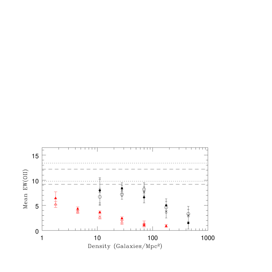
Figure 2.— Mean equivalent width of [Oii] versus projected local density. The mean EW([Oii] ) is computed over all galaxies. The high redshift points (EDisCS), described in §6.1, are shown in black as empty circles (statistical subtraction), filled circles (photo-z probable members) and crosses (photo-z within $\pm 0.1$ from $z_{clu}$). The low redshift points (SDSS), described in §6.4, are shown in red as empty triangles (density computed using only spectroscopic members) and filled triangles (full photometric catalog). Errors are computed as bootstrap standard deviations from the mean using 100 realizations. The horizontal dashed and dotted lines delimit the values found in the field and in poor groups at high redshift using mass-matched samples (see text).

                 

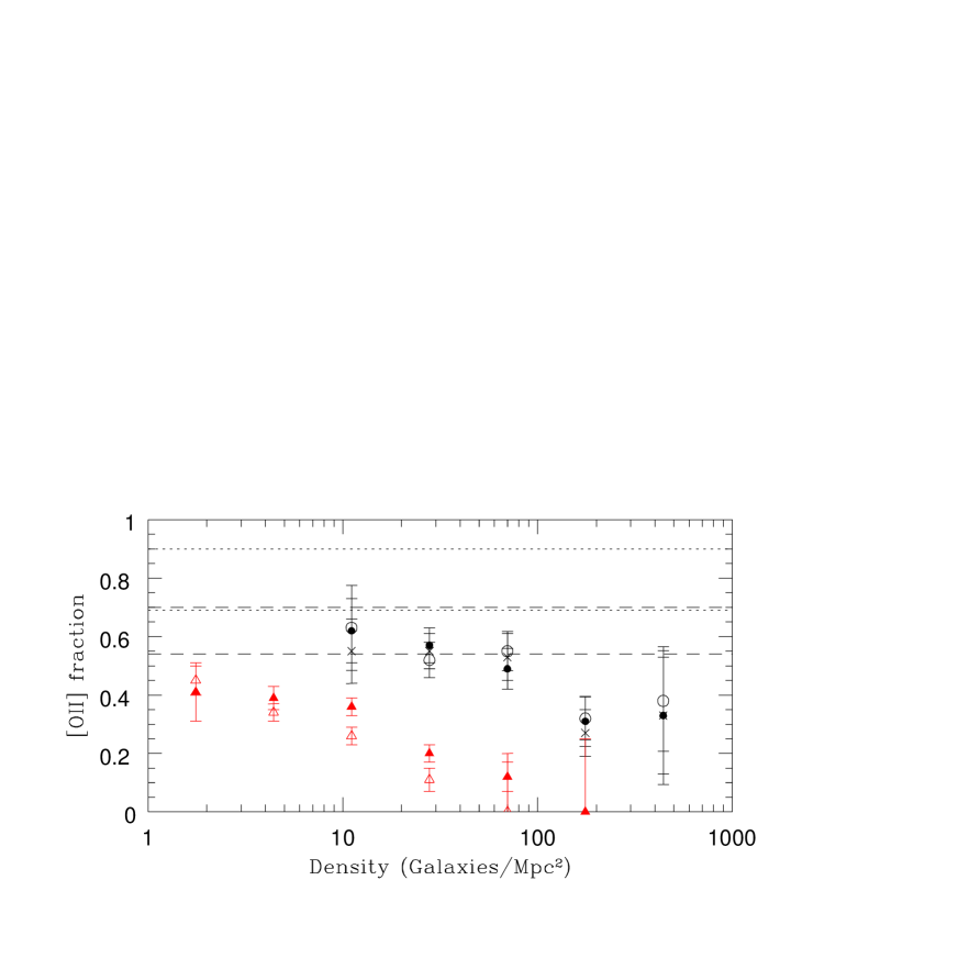
Figure 3.— Fraction of galaxies with [Oii] in emission versus local density. Symbols as in fig. 2. Black symbols (circles) are EDisCS points at $z=0.4-0.8$ (§6.1). Red symbols (triangles) are SDSS points at low redshift (§6.4). Errors on data points are computed from Poissonian statistics. The horizontal dashed and dotted lines delimit the value for field and poor group galaxies at $z=0.4-0.8$.

                 

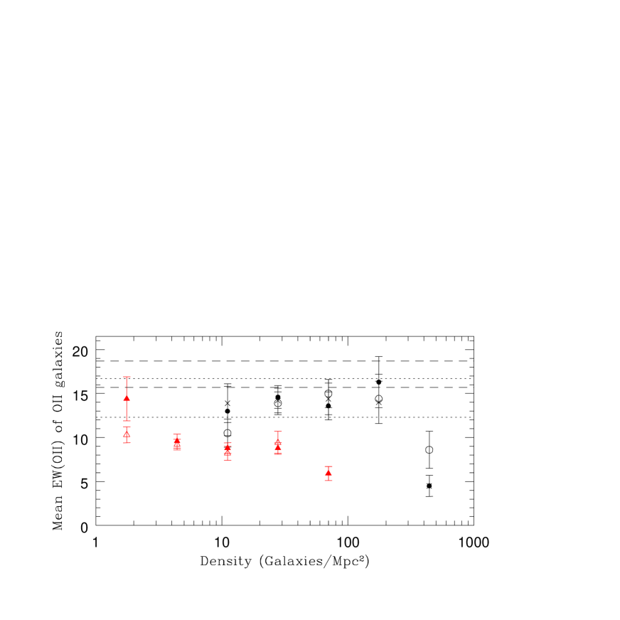
Figure 4.— The mean EW([Oii] ) only among galaxies with [Oii] in emission (EW$>3$ Å). Symbols as in fig. 2. Black symbols (circles) are EDisCS points at $z=0.4-0.8$ (§6.1). Red symbols (triangles) are SDSS points at low redshift (§6.4). Errors are computed as bootstrap standard deviations. The horizontal dashed and dotted lines delimit the value for mass-matched field and poor group galaxy samples at $z=0.4-0.8$.

                 

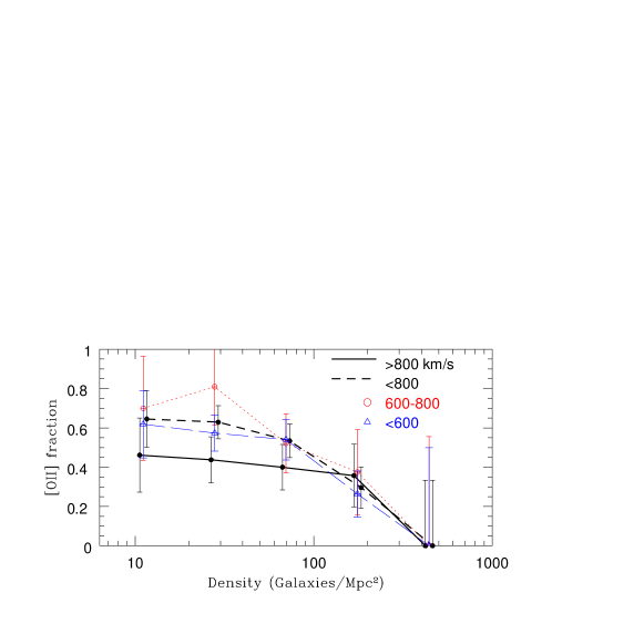
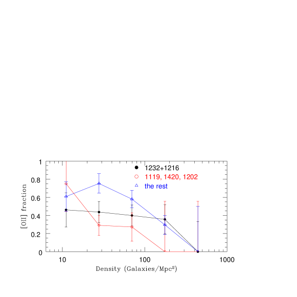
Figure 5.— Fraction of galaxies with [Oii] in emission versus local density for different subsets of our cluster sample: Left Clusters in different velocity dispersion bins: $\sigma>800\,\rm km\,s^{-1}$ (thick solid line) and $\sigma<800\,\rm km\,s^{-1}$ (thick dashed line). A small shift in density has been applied to allow a better visibility of the errors. The red dotted lines indicate clusters with $600<\sigma<800$ km s^-1 and blue, long-dashed lines respresent systems with $\sigma<600$ km s^-1. Right The two most massive clusters ($\sigma>800$ km s^-1, cl1232 and cl1216); the three outliers in the [OII]-$\sigma$ relation (cl1119, cl1420 and cl1202), and all the remaining clusters. Densities have been computed using the high-probability photometric-redshift membership (sec. 4).

                 

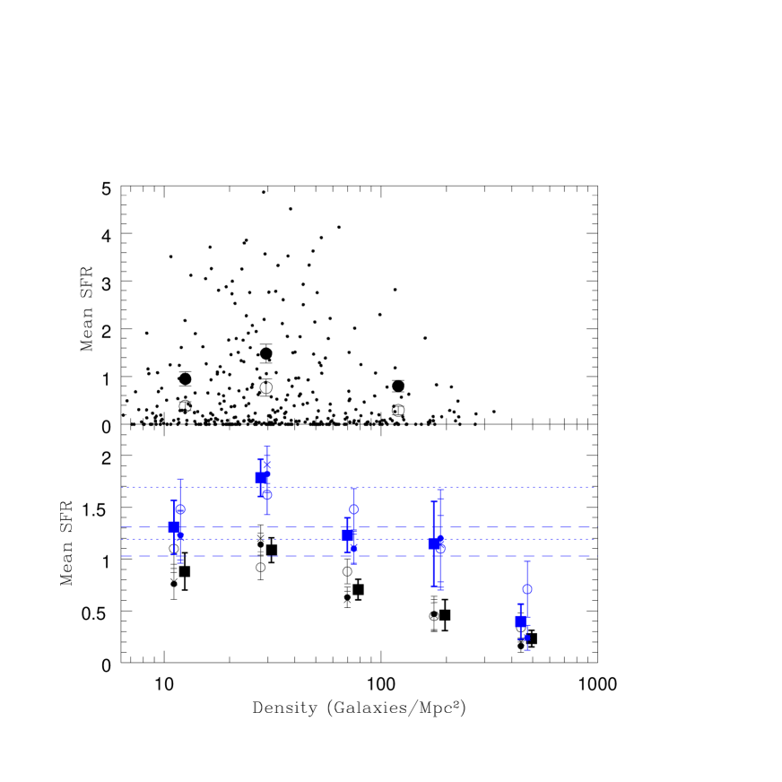
Figure 6.— Bottom Mean SFR in solar masses per year for galaxies in different density bins. All galaxies: black symbols. Only star-forming galaxies: blue symbols. Different symbols indicate the values obtained for the 3 membership criteria, as in Fig. 2. Large squares represent the average of the values for the 3 membership methods. A small shift around the center of each density bin has been applied to the different points to avoid confusion. The dashed and dotted lines delimit the 1$\sigma$ error around the value for field and group galaxies, respectively. For clarity, only the star-forming field and poor group values for the mass-matched samples are shown. Top SFR in solar masses per year for all individual galaxies. The mean (filled circles) and median (empty circles) SFR in star-forming galaxies are shown for three equally populated density bins (see text).

                 

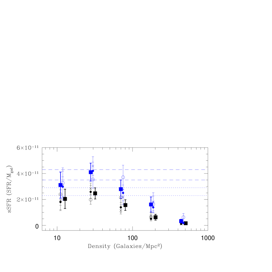
Figure 7.— Mean specific SFR (SFR/M, where M is the galaxy stellar mass) in $\rm yr^{-1}$ for galaxies in different density bins. All galaxies: black symbols. Only star-forming galaxies: blue symbols. Different symbols indicate the values obtained for the 3 membership criteria, as in Fig. 2. Large squares represent the average of the values for the 3 membership methods. A small shift around the center of each density bin has been applied to the different points to avoid confusion. The dashed and dotted lines delimit the 1$\sigma$ error around the value for field and group galaxies, respectively. For clarity, only the star-forming field and poor group values for the mass-matched samples are shown.

         

Figure 8.— Integrated cluster SFR per unit of cluster mass plotted as a function of cluster mass. The large cross identifies our lowest velocity dispersion group (Cl1119) whose SFR/Mass estimate is unreliable (see text). Left EDisCS clusters over a radius equal to $R_{200}$. Cl 1232 has not been included because observations cover only out to $=R_{200}/2$. Right EDisCS clusters (filled dots) and literature data (empty dots, see text) over a radius $=R_{200}/2$.

         

Figure 9.— Total integrated SFR as a function of cluster mass (right) and SFR/Mass versus fraction of star-forming galaxies (left). All quantities are computed within $R_{200}$. The large cross identifies our lowest velocity dispersion group (Cl1119) whose SFR/Mass estimate is unreliable (see text). Errors are computed by propagating errors on velocity dispersions and SFRs.

             

Figure 10.— Left Integrated cluster SFR versus number of star-forming cluster members (filled circles) and total number of cluster members (empty circles). The line represents the 1:1 relation, $SFR=N_{SF}$, which implies that the average SFR per star-forming galaxy is roughly equal to $1\rm\,M_{\odot}\,yr^{-1}$ in all clusters. Numbers are computed using spectroscopically-confirmed members and correcting for spectroscopic incompleteness. Error bars are omitted in this panel for clarity. All quantities are computed within $R_{200}$ to the galaxy magnitude limits adopted in this paper. Center Number of star-forming members versus cluster mass. Right Number of members within $R_{200}$ versus cluster mass. For EDisCS clusters, numbers are computed from photo-z membership (stars), statistical substraction (crosses) and from the number of spectroscopic members corrected for incompleteness (filled circles). The least squares fit for EDisCS clusters is shown as a solid line, and it is given in eqn. 1. Sloan clusters at low-z are shown as empty triangles, and the least squares fit as a dashed line (eqn. 3).

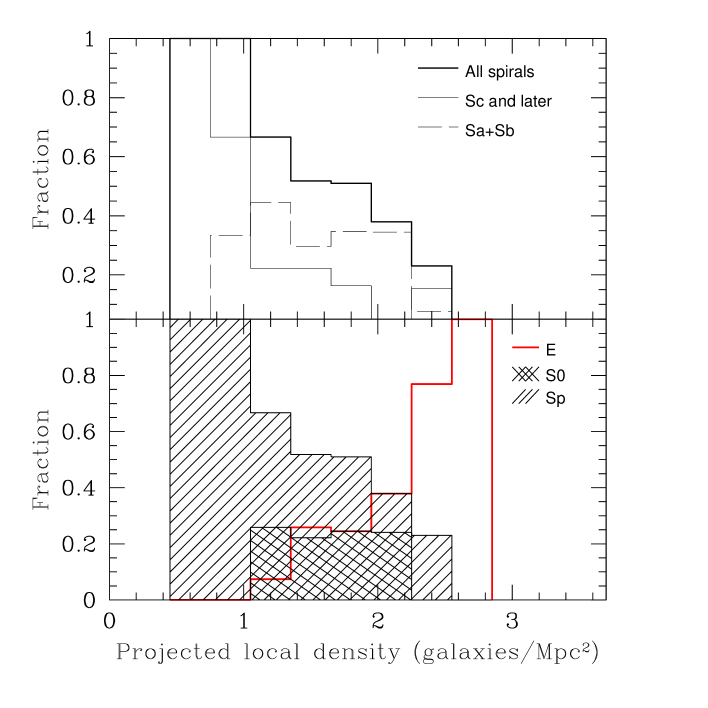
Figure 11.— Morphology-density relation for EDisCS spectroscopically-confirmed cluster members. Fraction of each morphological type in various density bins. Bottom Es: thick black histogram. S0: double shaded histogram. Spirals: single shaded histogram. Top All spirals: thick solid histogram. Early-type spirals (Sa’s and Sb’s): long-dashed histogram. Late-type spirals (Sc’s and later types): thin solid histogram. Note that the highest density bin is only populated by ellipticals.

         

Figure 12.— “Age-density” relation for galaxies of different morphological types. From left to right: SFR, [OII] equivalent width, D4000, and number of galaxies versus local density for (from bottom to top) Es, S0s, early spirals, and late spirals. The filled histogram shows the density distribution of “blue” early spirals with $D4000<1.3$.

                 

                 

Figure 13.— Fraction of star-forming galaxies (top) and mean SFR among all galaxies (bottom) with symbols as in Fig. 3 and Fig. 6. The large, solid squares represent the values expected given the morphology-density relation and the mean star-forming fraction and SFR of galaxies of each morphological class.

         

Figure 14.— Mean local density for each morphological type, from left to right: ellipticals, S0s, early spirals, and late spirals. The notation “old” and “young” here separates galaxies with red and blue D4000 ($>/<1.3$). Practically all ellipticals and S0s are old, and all late spirals are young, while early spirals are cleanly divided into two age populations with similar mean densities. Errors are bootstrap standard deviations.

References

- (1) Baldry, I.K., Balogh, M.L., Bower, R.G., Glazebrook, K., Nichol, R.C., Bamford, S.P., budavari, T., 2006, MNRAS, 373, 469
- (2) Ball, N.M., Loveday, J., Brunner, R.J, 2008, MNRAS in press (astro-ph 0610171)
- (3) Balogh, M.L., Morris, S.L., Yee, H.K.C., Carlberg, R.G., Ellingson, E., 1997, ApJ, 488, L75
- (4) Balogh, M.L., Morris, S.L., Yee, H.K.C., Carlberg, R.G., Ellingson, E., 1999, ApJ, 527, 54
- (5) Balogh, M.L., Eke, V., Miller, C., et al., 2004a, MNRAS, 348, 1355
- (6) Balogh, M.L., Baldry, I.K., Nichol, R., Miller, C., Bower, R., Glazebrook, K., 2004b, ApJ, 615, L101
- (7) Balogh, M.L., Wilman, D., Henderson, R.D.E., et al., 2007, MNRAS, 374, 1169
- (8) Bamford, S.P., Milvang-Jensen, B., Aragón-Salamanca, A., Simard, L., 2005, MNRAS, 361, 109
- (9) Bell. E., De Jong, R., 2001, ApJ, 550, 212
- (10) Blanton, M.R., Brinchmann, J., Csabai, I., Doi, M., Eisenstein, D., Fukugita, M., Gunn, J.E., Hogg, D.W., Schlegel, D.J., 2003, AJ, 125, 2348
- (11) Blanton, M.R., Eisenstein, D., Hogg, D.W., Schlegel, D.J., Brinchmann, J., 2005, ApJ, 629, 143
- (12) Bolzonella, M. Miralles, J.-M., Pelló, R., 2000, A&A, 363, 476
- (13) Brinchmann, J., Charlot, S., White, S.D.M., Tremonti, C., Kauffmann, G., Heckman, T., Brinkmann, J., 2004a, MNRAS, 351, 1151
- (14) Brinchmann et al. 2004b, astro-ph 0406220, announcement of data-release
- (15) Capak, P. et al. 2007, ApJS, 172, 284
- (16) Cassata, P. et al., 2007, ApJS, 172, 270
- (17) Clowe, D., et al., 2006, A&A, 451, 395
- (18) Cooper, M.C., Newman, J.A., Croton, J.A., et al., 2006, MNRAS, 370, 198
- (19) Cooper, M.C., Newman, J.A., Weiner, B.J., et al., 2007, MNRAS, 376, 1445
- (20) Cooper, M.C., Newman, J.A., Weiner, B.J., et al., 2008, MNRAS, in press (astro-ph 07064089)
- (21) Cucciati, O., Iovino, A., Marinoni, C., et al., 2006, A&A, 458, 39
- (22) Christlein, D., Zabludoff, A.I., 2005, ApJ, 621, 201
- (23) De Lucia, G., Poggianti, B.M., Aragón-Salamanca, A., et al., 2004, ApJ, 610, L77
- (24) De Lucia, G., Blaizot, J., 2007, MNRAS, 375, 2
- (25) De Lucia, G. et al., 2007, MNRAS, 374, 809
- (26) Desai, V., et al., 2007, ApJ, 660, 1151
- (27) Douglas, L.S., Bremer, M.N., Stanway, E., Lehnert, M., 2007, MNRAS, 376, 1393
- (28) Dressler, A. 1980, ApJ, 236, 351
- (29) Dressler, A., Oemler, A., Couch, W.J., Smail, I., Ellis, R.S., Barger, A., Butcher, H., Poggianti, B.M., Sharples, R.M., 1997, ApJ, 490, 577
- (30) Elbaz, D., Daddi, E., le Borgne, D., et al., 2007, A&A, 468, 33
- (31) Fasano, G., Poggianti, B. M., Couch, W. J., Bettoni, D., et al. 2000, ApJ, 542, 673
- (32) Feulner, G., Hopp, U., Botzler, C.S., 2006, A&A, 451, L13
- (33) Finn, R.A., Zaritsky, D., McCarthy, D.W., Poggianti, B.M., Rudnick, G., Halliday, C., Milvang-Jensen, B., Pelló, R., Simard, L., 2005, ApJ, 630, 206
- (34) Finn, R.A., Balogh, M.L., Zaritsky, D., Miller, C.J., Nichol, R.C., 2008, ApJ in press (astro-ph 0802.2282)
- (35) Finoguenov, A., et al., 2007, ApJS, 172, 182
- (36) Gao, L, Navarro, J.F., Cole, S., Frenk, C.S., White, S.D.M., Springel, V., Jenkins, A., Neto, A.F., 2008, MNRAS in press (astro-ph 0711.0746)
- (37) Geach, J.E., Smail, I., Ellis, R.S., Moran, S.M., Smith, G.P., Treu, T., Kneib, J.-P., Edge, A.C., Kodama, T., 2006, ApJ, 649, 661
- (38) Gerke, B.F. et al., 2005, ApJ, 625, 6
- (39) Gerke, B.F., Newman, J.A., Faber, S.M., et al. 2007, MNRAS, 376, 1425
- (40) Gilbank, D.G., Yee, H.K.C., Ellingson, E., Gladders, M.D., Loh, Y.-S., Barrientos, L.F., Barkhouse, W.A., 2008, ApJ, in press (astro-ph 07102351)
- (41) Gomez, P.L., Nichol, R.C., Miller, C.J., et al., 2003, ApJ, 584, 210
- (42) Gonzalez, A.H., Zaritsky, D., Dalcanton, J.J., Nelson, A., 2001, ApJS, 137, 117
- (43) Goto, T., et al., 2003, PASJ, 55, 757
- (44) Halliday, C. et al., 2004, A&A, 427, 397
- (45) Hashimoto, Y., Oemler, A., Lin, H., Tucker, D.L., 1998, ApJ, 499, 589
- (46) Hicks, A.K., Ellingson, E., Bautz, M., Cain, B., Gilbank, D.G., Gladders, M.G., Hoekstra, H., Yee, H.K.C., Garmire, G., 2008, ApJ in press (astro-ph 07105513)
- (47) Hogg, D.W., et al., 2004, ApJ, 601, L29
- (48) Homeier, N.L., et al., 2005, ApJ, 621, 651
- (49) Hubble, E., Humason, M.L., 1931, ApJ, 74, 43
- (50) Johnson, O. et al., 2006, MNRAS, 371, 1777
- (51) Kauffmann, G., White, S.D., Heckman, T.M., Menard, B., Brinchmann, J., Charlot, S., Tremonti, C., Brinkmann, J, 2004, MNRAS, 353, 713
- (52) Kewley, L.J., Geller, M.J., jansen, R.A., 2004, AJ, 127, 2002
- (53) Kodama, T., Balogh, M.L., Smail, I., Bower, R.G., Nakata, F., 2004, MNRAS, 354, 1103
- (54) Lewis, I., Balogh, M., De Propris, R. et al., 2002, MNRAS, 334, 67
- (55) Milvang-Jensen, B., Aragón-Salamanca, A., Hau, G.K.T., Jorgensen, I., Hjorth, J., 2003, MNRAS, 339, 1
- (56) Milvang-Jensen, B., et al., 2008, A&A in press (astro-ph 0802.0149)
- (57) Moran, S.M., Ellis, R.S., Treu, T., Smail, I., Dressler, A., Coil, A.L., Smith, G.P., 2005, ApJ, 634, 977
- (58) Moran, S.M., Ellis, R.S., Treu, T., Salim, S., Rich, R.M., Smith, G.P., Kneib, J.-P., 2006, ApJL, 641, L97
- (59) Moran, S.M., Ellis, R.S., Treu, T., Smith, G.P., Rich, R.M., Smail, I., 2007, ApJ, 671, 1503
- (60) Moustakas, J., Kennicutt, R., Tremonti, C.A., 2006, ApJ, 642, 775
- (61) Park, C., Choi, Y.-Y., Vogeley, M.S., Gott, R., Blanton, M.R., 2007, ApJ, 658, 898
- (62) Pimbblet, K.A., Smail, I., Kodama, T., Couch, W.J., Edge, A.C., Zabludoff, A.I., O’Hely, E., 2002, MNRAS, 331 333
- (63) Poggianti, B. M., Smail, I., Dressler, A., Couch, W. J., Barger, A. J., Butcher, H., et al. 1999, ApJ, 518, 576
- (64) Poggianti, B.M., Bridges, T.J., Mobasher, B. et al., 2001a, ApJ, 562, 689
- (65) Poggianti, B.M., Bridges, T.J., Carter, D. et al., 2001b, ApJ, 563, 118
- (66) Poggianti, B.M., Bridges, T.J., Komiyama, Y. et al., 2004, ApJ, 601, 197
- (67) Poggianti, B.M., et al., 2006, ApJ, 642, 188
- (68) Postman, M., Geller, M.J., 1984, ApJ, 281, 95
- (69) Postman, M., Lauer, T.R., Szapudi, I., Oegerle, W., 1998, ApJ, 506, 33
- (70) Postman, M. et al., 2005, ApJ, 623, 721
- (71) Rudnick, G., Franx, M., Rix, H.-W., Moorwood, A., Kuijken, K., van Starkenburg, L., van der Werf, P., Rottgering, H., Labbe’ I., 2001, AJ, 122, 2205
- (72) Rudnick, G., et al., 2003, ApJ, 599, 847
- (73) Simard, L., et al., 2008, A&A, in press
- (74) Smail, I., Edge, A.C., Ellis, R. S., Blandford, R.D., 1998, MNRAS, 293, 124
- (75) Smith, G.P., Treu. T., Ellis, R.S., Moran, S.M., Dressler, A., 2005, ApJ, 620, 78
- (76) Spitzer, L., Baade, W., a951, ApJ, 113, 413
- (77) Springel, V., White, S.D.M., Jenkins, A., et al. 2005, Nature, 435, 629
- (78) Treu, T., Ellis, R.S., Kneib, J.-P., Dressler, A., Smail, I., Czoske, O., Oemler, A., Natarajan, P., 2003, ApJ, 591, 53
- (79) van der Wel, A., 2008, ApJL, in press (astro-ph 08011995)
- (80) Whiley, I., et al., 2008, MNRAS, in press (astro-ph ???)
- (81) White, S.D.M., Clowe, D., I., Simard, L., et al. 2005, A&A, 444, 365
- (82) Wilman, D.J., Balogh, M.L., Bower, R.G., Mulchaey, J.S., Oemler, A., Carlberg, R.G., Morris, S.L., Whitaker, R.J., 2005, MNRAS, 358, 71
- (83) Wolf, C., Gray, M.E., Aragón-Salamanca, A., Lane, K.P., Meisenheimer, K, 2007, MNRAS, L1
- (84) Yan, R., Newman, J.A., Faber, S.M.,. Konidaris, N., Koo, D., Davis, M., 2006, ApJ, 648, 281