A Chebyshev criterion for Abelian integrals

Abstract

We present a criterion that provides an easy sufficient condition in order that a collection of Abelian integrals has the Chebyshev property. This condition involves the functions in the integrand of the Abelian integrals and can be checked, in many cases, in a purely algebraic way. By using this criterion, several known results are obtained in a shorter way and some new results, which could not be tackled by the known standard methods, can also be deduced.

1 Introduction and statement of the result

The second part of Hilbert’s 16th problem [15] asks about the maximum number and location of limit cycles of a planar polynomial vector fields of degree $d.$ Solving this problem, even in the case $d=2,$ seems to be out of reach at the present state of knowledge (see the works of Ilyashenko [17] and Li Jibin [20] for a survey of the recent results on the subject). Our paper is concerned with a weaker version of this problem, the so-called infinitesimal Hilbert’s 16th problem, proposed by Arnold [1]. Let $\omega$ be a real 1-form with polynomial coefficients of degree at most $d.$ Consider a real polynomial $H$ of degree $d+1$ in the plane. A closed connected component of a level curve $H=h$ is denoted by $\gamma_{h}$ and called an oval of $H.$ These ovals form continuous families (see Figure 2) and the infinitesimal Hilbert’s 16th problem is to find an upper bound $V(d)$ of the number of real zeros of the Abelian integral

(1) $$I(h)=\int_{\gamma_{h}}\omega.$$

The bound should be uniform with respect to the choice of the polynomial $H,$ the family of ovals $\{\gamma_{h}\}$ and the form $\omega.$ It should depend on the degree $d$ only. (In the literature an Abelian integral is usually the integral of a rational 1-form over a continuous family of algebraic ovals. Throughout the paper, by an abuse of language, we use the name Abelian integral also in case the functions are analytic.)

Zeros of Abelian integrals are related to limit cycles in the following way. Consider a small deformation of a Hamiltonian vector field $X_{\varepsilon}=X_{H}+\varepsilon Y,$ where

$$X_{H}=-H_{y}\partial_{x}+H_{x}\partial_{x}\,\mbox{ and }\,Y=P\partial_{x}+Q\partial_{y}.$$

Then, see [17, 20] for details, the first approximation in $\varepsilon$ of the displacement function of the Poincaré map of $X_{\varepsilon}$ is given by $(\ref{Abeliana})$ with $\omega=Pdy-Qdx.$ Hence the number of isolated zeros of $I(h),$ counted with multiplicities, provides an upper bound for the number of ovals of $H$ that generate limit cycles of $X_{\varepsilon}$ for $\varepsilon\approx 0.$ The coefficients of $P$ and $Q$ are considered as parameters of the problem and so the function $I(h)$ splits as a linear combination

$$\alpha_{0}I_{0}(h)+\alpha_{1}I_{1}(h)+\ldots+\alpha_{n-1}I_{n-1}(h),$$

where $\alpha_{k}$ depends on the initial parameters and $I_{k}(h)$ is an Abelian integral with either $\omega=x^{i}y^{j}dx$ or $\omega=x^{i}y^{j}dy$. (In fact it is easy to see, using integration by parts, that only one type of these 1-forms needs to be considered.) Therefore the problem is equivalent to find an upper bound for the number of isolated zeros of any function belonging to the vector space generated by $I_{k}(h)$ for $k=0,1,\ldots,n-1.$ This problem is strongly related to showing that the basis of the previous vector space is a Chebyshev system. In fact, the great majority of papers studying concrete problems on the subject show this kind of property.

In this paper we focus on the case in which $H$ has separated variables, i.e., $H(x,y)=\Phi(x)+\Psi(y),$ and as a byproduct we obtain a result for the case $H(x,y)=A(x)+B(x)y^{2m}$ as well. We suppose in addition that

$$I_{i}(h)=\int_{\gamma_{h}}f_{i}(x)g(y)dx,\ \mbox{ for $i=0,1,\ldots,n-1,$}$$

where $f_{0},f_{1},\ldots,f_{n-1}$ and $g$ are analytic functions. (Note that the function depending on $y$ is the same for all the 1-forms. In the problems studied in the literature, the original family of Abelian integrals can be usually reduced to a family as above.) We will show that, in this case, some Chebyshev properties on $f_{i}$ and $g$ (to be specified later on) transfer to $I_{i}$ after the integration over the ovals. To fix notation, $H$ is an analytic function in some open subset of the plane that has a local minimum at the origin. Then there exists a punctured neighbourhood $\mathcal{P}$ of the origin foliated by ovals $\gamma_{h}\subset\{H(x,y)=h\}.$ We fix that $H(0,0)=0$ and then the set of ovals $\gamma_{h}$ inside this, let us say, period annulus, can be parameterized by the energy levels $h\in(0,h_{0})$ for some $h_{0}\in(0,+\infty]$. In what follows, we shall denote the projection of $\mathcal{P}$ on the $x$-axis by $(x_{\ell},x_{r})$. Similarly, $(y_{\ell},y_{r})$ is the projection of $\mathcal{P}$ on the $y$-axis.

Theorem A is our main result and it applies in case that $H(x,y)=\Phi(x)+\Psi(y).$ It is easy to verify that, under the above assumptions, $x\Phi^{\prime}(x)>0$ for any $x\in(x_{\ell},x_{r})\setminus\{0\}$ and $y\Psi^{\prime}(y)>0$ for any $y\in(y_{\ell},y_{r})\setminus\{0\}.$ Then $\Phi$ and $\Psi$ must have even multiplicity at $0.$ Thus, there exist two analytic involutions $\sigma_{1}$ and $\sigma_{2}$ such that

$$\Phi(x)=\Phi\bigl{(}\sigma_{1}(x)\bigr{)} x\in(x_{\ell},x_{r})$$ for all

and

$$\Psi(y)=\Psi\bigl{(}\sigma_{2}(y)\bigr{)} y\in(y_{\ell},y_{r}).$$ for all

Recall that a mapping $\sigma$ is an involution if $\sigma\circ\sigma=Id$ and $\sigma\neq Id.$ Note that an involution is a diffeomorphism with a unique fixed point. In our situation we have that $\sigma_{i}(0)=0.$ In what follows, given a function $\kappa,$ we define its balance with respect to $\sigma$ as

$$\mathscr{B}_{\sigma}\!\bigl{(}\kappa\bigr{)}(x)=\kappa(x)-\kappa\bigl{(}\sigma(x)\bigr{)}.$$

For example, if $\sigma=-Id$, then the balance of a function is twice its odd part.

In the statement of Theorem A, $m$ is related with the multiplicity of $\Psi$ at $y=0.$ More concretely, we suppose that $\Psi(y)=ey^{2m}+\mbox{\rm o}(y^{2m})$ with $e>0.$ In addition, ECT-system stands for extended complete Chebyshev system in the sense of Mardešić [22], see Definition 2 for details.

Theorem A.

Let us consider the Abelian integrals

$$I_{i}(h)\,=\,\int_{\gamma_{h}}f_{i}(x)g(y)dx,\ \mbox{ $i=0,1,\ldots,n-1,$}$$

where, for each $h\in(0,h_{0}),$ $\gamma_{h}$ is the oval surrounding the origin inside the level curve $\{\Phi(x)+\Psi(y)=h\}.$ Let $\sigma_{1}$ and $\sigma_{2}$ be the involutions associated to $\Phi$ and $\Psi$, respectively. Setting $g_{0}=g,$ we define $g_{i+1}=\frac{g^{\prime}_{i}}{\Psi^{\prime}}$. Then $(I_{0},I_{1},\ldots,I_{n-1})$ is an ECT-system on $(0,h_{0})$ if the following hypothesis are satisfied:

1. $\Bigl{(}\mathscr{B}_{\sigma_{1}}\!\bigl{(}\frac{f_{0}}{\Phi^{\prime}}\bigr{)},\mathscr{B}_{\sigma_{1}}\!\bigl{(}\frac{f_{1}}{\Phi^{\prime}}\bigr{)},\ldots,\mathscr{B}_{\sigma_{1}}\!\bigl{(}\frac{f_{n-1}}{\Phi^{\prime}}\bigr{)}\Bigr{)}$ is a CT-system on $(0,x_{r}),$ and

2. $\Bigl{(}\mathscr{B}_{\sigma_{2}}\!(g_{0}),\mathscr{B}_{\sigma_{2}}\!(g_{1}),\ldots,\mathscr{B}_{\sigma_{2}}\!(g_{n-1})\Bigr{)}$ is a CT-system on $(0,y_{r})$ and $\mathscr{B}_{\sigma_{2}}\!(g_{0})(y)=\mbox{\rm o}(y^{2m(n-2)}).$

To prove the result it is necessary to compute the derivative of each Abelian integral until order $n-1$. The condition on $\mathscr{B}_{\sigma_{2}}\!(g_{0})(y)$ at $y=0$ ensures that the integral expression of this derivative is convergent, although it may be improper (see Remark 3). Let us also point out that, since $\sigma_{2}(y)=-y+\mbox{\rm o}(y),$ this condition is equivalent to require that $g(y)-g(-y)=\mbox{\rm o}(y^{2m(n-2)}).$

Our second result deals with those Abelian integrals such that

$$H(x,y)=A(x)+B(x)y^{2m}\ \mbox{ and $g(y)=y^{2s-1}$ with $s\in\mathbb{N}.$}$$

Since $H$ has a local minimum at the origin by assumption, $B(0)>0$ and $A$ has a local minimum at $x=0.$ Thus, as before, there exists an involution $\sigma$ satisfying $A(x)=A\bigl{(}\sigma(x)\bigr{)}$ for all $x\in(x_{\ell},x_{r})$.

Theorem B.

Let us consider the Abelian integrals

$$I_{i}(h)=\int_{\gamma_{h}}f_{i}(x){y^{2s-1}}dx,\ \mbox{ $i=0,1,\ldots,n-1,$}$$

where, for each $h\in(0,h_{0}),$ $\gamma_{h}$ is the oval surrounding the origin inside the level curve $\{A(x)+B(x)y^{2m}=h\}.$ Let $\sigma$ be the involution associated to $A$ and we define

$$\textstyle{\ell_{i}=\mathscr{B}_{\sigma}\!\left(\frac{f_{i}}{A^{\prime}B^{\frac{2s-1}{2m}}}\right).}$$

Then $(I_{0},I_{1},\ldots,I_{n-1})$ is an ECT-system on $(0,h_{0})$ if $s>m(n-2)$ and $\bigl{(}\ell_{0},\ell_{1},\ldots,\ell_{n-1}\bigr{)}$ is a CT-system on $(0,x_{r}).$

It is worth noting that although the condition $s>m(n-2)$ is not fulfilled in some situations, it is possible to obtain a new Abelian integral for which the corresponding $s$ is large enough to verify the inequality. The procedure to obtain this new Abelian integral follows from the application of Lemma 4.1. We refer the reader to Example 4 in which we explain in detail how to apply Lemma 4.1 to get a new Abelian integral with $s>m(n-2)$.

The applicability of our criteria comes from the fact that the hypothesis requiring some functions to be a CT-system can be verified by computing Wronskians (see Lemma 2.3). This simplifies a lot the problem of showing that a given collection of Abelian integrals has the Chebyshev property and in some cases it enables to reformulate the problem in a purely algebraic way (cf. Section 4).

In the literature there are a lot of papers dealing with zeros of Abelian integrals (see for instance [5, 6, 9, 10, 14, 23, 24] and references there in). In many cases, it is essential to show that a collection of Abelian integral has some kind of Chebyshev property. The techniques and arguments to tackle these problems are usually very long and highly non-trivial. For instance, in some papers (e.g. [4, 7, 21]) the authors study the geometrical properties of the so-called centroid curve using that it verifies a Riccati equation (which is itself deduced from a Picard-Fuchs system). In other papers (e.g. [8, 12, 13]), the authors use complex analysis and algebraic topology (analytic continuation, argument principle, monodromy, Picard-Lefschetz formula, …). Certainly, the criterion that we present here can not be applied to all the situations (since the Abelian integrals need to have a specific structure) and, even in case that it is possible to apply it, sometimes the sufficient condition that we provide is not verified. However we want to stress that, when it works, it enables to extremely simplify the solution. To illustrate this fact, in Section 4 we reprove with our criterion the main results of three different papers. We are also convinced that this criterion will be useful to obtain new results on the issue. In this direction we tackle the program posed by Gautier, Gavrilov and Iliev [8] and we prove their conjecture in four new cases (see Subsection 4.1).

In several papers dealing with zeros of Abelian integrals (see [2, 3, 4, 21] for instance), it is applied a criterion of Li and Zhang [19]. This criterion provides a sufficient condition for the monotonicity of the ratio of two Abelian integrals. In page 360 of the book of Arnold’s problems [1], the criterion given in [19] is quoted as a useful tool that “despite its seemingly artificial form, it proves to be working in many independently arising particular cases”. The translation of the result in [19] to the language of Chebyshev systems and Wronskians shows that it corresponds precisely to the case $n=2$ of our criteria. Accordingly, using our formulation, their result becomes very natural: it shows that the Chebyshev properties of the functions in the 1-form are preserved after integration. In addition, as a generalization of their result, we hope that our criteria will be useful in many cases as well. Finally we remark that, although we suppose that the functions that we deal with are analytic, our results hold true for smooth functions with minor changes.

The paper is organized as follows. Section 2 is devoted to introduce the definitions and the notation that we shall use. In particular we define the different types of Chebyshev property that we shall deal with and we establish their equivalences with the continuous and discrete Wronskians (see Lemma 2.3). Theorems A and B are proved in Section 3. The main ingredient in the proof of Theorem A is Proposition 3.3, that provides an integral expression for the Wronskian of a collection of Abelian integrals. Theorem B follows as a corollary of Theorem A. Section 4 is devoted to illustrate the application of our criteria. To this end, in Examples 4, 4 and 4 we reprove the results of Iliev and Perko [8], Zhao, Liang and Lu [24] and Peng [21], respectively. Apart from showing the simplicity in the application of the criteria, our aim with these examples is twofold. First, to show that it is not necessary to know explicitly the involutions that appear in the statements. Second, to show that it is possible to reformulate the problem in such a way it suffices to check that some polynomials do not vanish. In Section 4 we also present some new results concerning the program of Gautier, Gavrilov and Iliev [8]. Finally in the Appendix we give some details about the tools that are used in Section 4, namely, the notion of resultant between two polynomials and Sturm’s Theorem.

2 Chebyshev systems

• Let $f_{0},f_{1},\ldots,f_{n-1}$ be analytic functions on an open interval $L$ of $\mathbb{R}.$

  1. $(f_{0},f_{1},\ldots,f_{n-1})$ is a Chebyshev system $($in short, T-system$)$ on $L$ if any nontrivial linear combination

     $$\alpha_{0}f_{0}(x)+\alpha_{1}f_{1}(x)+\ldots+\alpha_{n-1}f_{n-1}(x)$$

     has at most $n-1$ isolated zeros on $L.$

  2. $(f_{0},f_{1},\ldots,f_{n-1})$ is a complete Chebyshev system $($in short, CT-system$)$ on $L$ if $(f_{0},f_{1},\ldots,f_{k-1})$ is a T-system for all $k=1,2,\ldots,n.$

  3. $(f_{0},f_{1},\ldots,f_{n-1})$ is an extended complete Chebyshev system $($in short, ECT-system$)$ on $L$ if, for all $k=1,2,\ldots,n,$ any nontrivial linear combination

     $$\alpha_{0}f_{0}(x)+\alpha_{1}f_{1}(x)+\ldots+\alpha_{k-1}f_{k-1}(x)$$

     has at most $k-1$ isolated zeros on $L$ counted with multiplicities.

  (Let us mention that, in these abbreviations, “T” stands for Tchebycheff, which in some sources is the transcription of the Russian name Chebyshev.) $\square$

It is clear that if $(f_{0},f_{1},\ldots,f_{n-1})$ is an ECT-system on $L$, then $(f_{0},f_{1},\ldots,f_{n-1})$ is a CT-system on $L$. However, the reverse implication is not true.

• Let $f_{0},f_{1},\ldots,f_{k-1}$ be analytic functions on an open interval $L$ of $\mathbb{R}.$ The continuous Wronskian of $(f_{0},f_{1},\ldots,f_{k-1})$ at $x\in L$ is

  $$W\bigl{[}f_{0},f_{1},\cdots,f_{k-1}\bigr{]}(x)=\det\left(f_{j}^{(i)}(x)\right)_{0\leqslant i,j\leqslant k-1}=\left|\begin{array}[]{ccc}f_{0}(x)&\cdots&f_{k-1}(x)\\ f^{\prime}_{0}(x)&\cdots&f^{\prime}_{k-1}(x)\\ &\vdots&\\ f^{(k-1)}_{0}(x)&\cdots&f^{(k-1)}_{k-1}(x)\\ \end{array}\right|$$

  The discrete Wronskian of $(f_{0},f_{1},\ldots,f_{k-1})$ at $(x_{0},x_{1},\ldots,x_{k-1})\in L^{k}$ is

  $$D\bigl{[}f_{0},f_{1},\cdots,f_{k-1}\bigr{]}(x_{0},x_{1},\ldots,x_{k-1})=\det\bigl{(}f_{j}(x_{i})\bigr{)}_{0\leqslant i,j\leqslant k-1}=\left|\begin{array}[]{ccc}f_{0}(x_{0})&\cdots&f_{k-1}(x_{0})\\ f_{0}(x_{1})&\cdots&f_{k-1}(x_{1})\\ &\vdots&\\ f_{0}(x_{k-1})&\cdots&f_{k-1}(x_{k-1})\\ \end{array}\right|$$

  $\square$

For the sake of shortness, given any “letter” $x$ and $k\in\mathbb{N}$ we use the notation

$$x_{0},x_{1},\ldots,x_{k-1}=\mathbf{x_{k}}.$$

Accordingly, we write

$$W\bigl{[}f_{0},f_{1},\cdots,f_{k-1}\bigr{]}(x)=W\bigl{[}\mathbf{f_{k}}\bigr{]}(x)$$

and

$$D\bigl{[}f_{0},f_{1},\cdots,f_{k-1}\bigr{]}(x_{0},x_{1},\ldots,x_{k-1})=D\bigl{[}\mathbf{f_{k}}\bigr{]}(\mathbf{x_{k}})$$

for the continuous and discrete Wronskian, respectively. The following result is well known (see [18, 22] for instance).

Lemma 2.3.

The following equivalences hold:

1. $(f_{0},f_{1},\ldots,f_{n-1})$ is a CT-system on $L$ if, and only if, for each $k=1,2,\ldots,n,$

   $$D\bigl{[}\mathbf{f_{k}}\bigr{]}(\mathbf{x_{k}})\neq 0\,\mbox{ for all $\mathbf{x_{k}}\in L^{k}$ such that $x_{i}\neq x_{j}$ for $i\neq j.$}$$

2. $(f_{0},f_{1},\ldots,f_{n-1})$ is an ECT-system on $L$ if, and only if, for each $k=1,2,\ldots,n,$

   $$W\bigl{[}\mathbf{f_{k}}\bigr{]}(x)\neq 0\mbox{ for all $x\in L.$}$$

3 Proof of the main results

The first part of this section is devoted to prove Theorem A. Thus, unless we explicitly say the contrary, we suppose that $H(x,y)=\Phi(x)+\Psi(y)$, where $\Psi(y)=ey^{2m}+\mbox{\rm o}(y^{2m})$ with $e>0$, as mentioned before. Then, there exists a diffeomorphism $\beta$ on $(y_{\ell},y_{r})$ such that

$$\textstyle{\Psi(y)=\frac{1}{2m}\,\beta(y)^{2m}.}$$

We take this diffeomorphism into account and we can write the involution associated to $\Psi$ as

$$\sigma_{2}(y)=\beta^{-1}\bigl{(}-\beta(y)\bigr{)}.$$

In what follows, for each $h\in(0,h_{0})$, we denote the projection of the oval $\gamma_{h}$ on the $x$-axis by $(x_{h}^{-},x_{h}^{+}).$ Therefore, $x_{\ell}<x_{h}^{-}<0<x_{h}^{+}<x_{r}$ and $\Phi(x_{h}^{\pm})=h.$

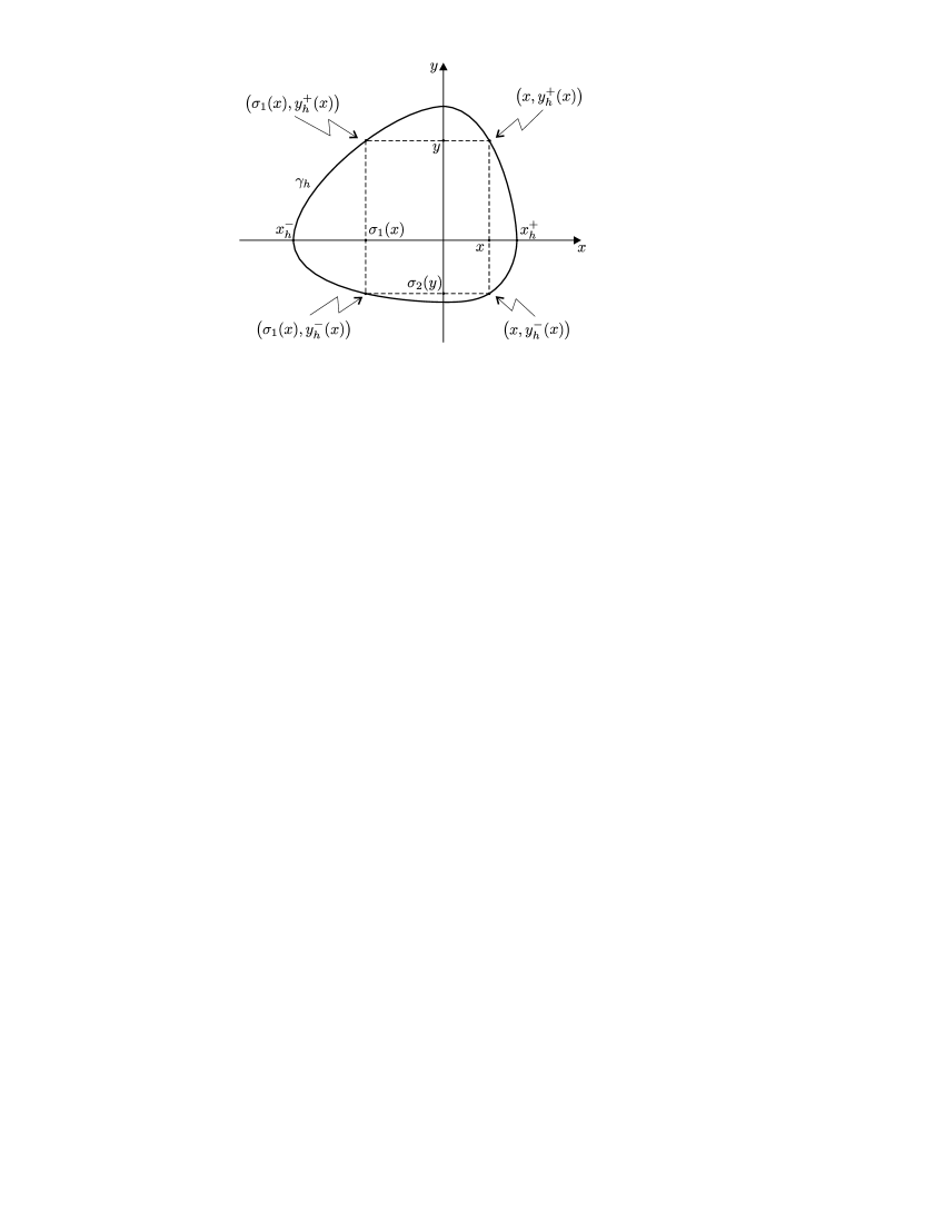
Figure 1: Notation related to the oval $\gamma_{h}$.

Moreover (see Figure 1), if $(x,y)\in\gamma_{h},$ then

$$y=y_{h}^{+}(x)\,\mbox{ for $y>0$ and }y=y_{h}^{-}(x)\,\mbox{ for $y<0,$}$$

where

$$y_{h}^{\pm}(x)\!:=\beta^{-1}\left(\pm\sqrt[2m]{2m\bigl{(}h-\Phi(x)\bigr{)}}\right).$$

We note that $y_{h}^{\pm}(x)=y_{h}^{\pm}\bigl{(}\sigma_{1}(x)\bigr{)},$ where we recall that $\sigma_{1}$ is the involution associated to $\Phi.$ We begin by the proof of the following result.

Lemma 3.1.

Let $f$ and $g$ be analytic functions on $(x_{\ell},x_{r})$ and $(y_{\ell},y_{r})$, respectively, and let us consider

$$I(h)=\int_{\gamma_{h}}f(x)g(y)dx.$$

We set $\ell(x)\!:=f(x)-f\bigl{(}\sigma_{1}(x)\bigr{)}\sigma^{\prime}_{1}(x)$ and $\xi_{k}\!:=\mathscr{B}_{\sigma_{2}}(g_{k}),$ where $g_{k}$ is recursively defined by means of $g_{k+1}=\frac{g^{\prime}_{k}}{\Psi^{\prime}}$ with $g_{0}=g.$ Then, if $\xi_{0}(y)=\mbox{\rm o}\bigl{(}y^{2m(n-2)}\bigr{)},$

$$I^{(k)}(h)=\int_{0}^{x_{h}^{+}}\ell(x)\,\xi_{k}\bigl{(}y_{h}^{+}(x)\bigr{)}dx\ \mbox{ for $k=0,1,\ldots,n-1.$}$$

• We prove the result by induction on $k.$ We take the parameterization of the oval $\gamma_{h}$ given by the mappings $x\longmapsto\bigl{(}x,y_{h}^{\pm}(x)\bigr{)}$, with the clockwise orientation, and we use $y_{h}^{-}(x)=\sigma_{2}\bigl{(}y_{h}^{+}(x)\bigr{)},$ to get that

  $$I(h)= \int_{x_{h}^{+}}^{x_{h}^{-}}f(x)g\bigl{(}y_{h}^{-}(x)\bigr{)}dx+\int_{x_{h}^{-}}^{x_{h}^{+}}f(x)g\bigl{(}y_{h}^{+}(x)\bigr{)}dx=\int_{x_{h}^{-}}^{x_{h}^{+}}f(x)\left.\bigl{(}g(y)-g(\sigma_{2}(y))\bigr{)}\right|_{y=y_{h}^{+}(x)}dx$$

  $$= \int_{x_{h}^{-}}^{0}f(x)\left.\bigl{(}g(y)-g(\sigma_{2}(y))\bigr{)}\right|_{y=y_{h}^{+}(x)}dx+\int_{0}^{x_{h}^{+}}f(x)\left.\bigl{(}g(y)-g(\sigma_{2}(y))\bigr{)}\right|_{y=y_{h}^{+}(x)}dx$$

  $$= \int_{x_{h}^{+}}^{0}f\bigl{(}\sigma_{1}(u)\bigr{)}\sigma_{1}^{\prime}(u)\left.\bigl{(}g(y)-g(\sigma_{2}(y))\bigr{)}\right|_{y=y_{h}^{+}(\sigma_{1}(u))}du+\int_{0}^{x_{h}^{+}}f(x)\left.\bigl{(}g(y)-g(\sigma_{2}(y))\bigr{)}\right|_{y=y_{h}^{+}(x)}dx,$$

  where in the last equality we performed the change of variable $x=\sigma_{1}(u).$ Thus, since $y_{h}^{+}(\sigma_{1}(u))=y_{h}^{+}(u),$ the above expression yields to

  $$I(h)=\int_{0}^{x_{h}^{+}}\bigl{(}f(x)-f(\sigma_{1}(x))\sigma_{1}^{\prime}(x)\bigr{)}\left.\bigl{(}g(y)-g(\sigma_{2}(y))\bigr{)}\right|_{y=y_{h}^{+}(x)}dx=\int_{0}^{x_{h}^{+}}\ell(x)\mathscr{B}_{\sigma_{2}}\bigl{(}g\bigr{)}\bigl{(}y_{h}^{+}(x)\bigr{)}dx.$$

  This expression proves the result for $k=0.$ We assume now that the result holds true for $k<n-1.$ On account of the hypothesis about the order of $\xi_{0}$ at $y=0,$ an easy computation shows that $\xi_{k}(y)=\mathscr{B}_{\sigma_{2}}\bigl{(}g_{k}\bigr{)}(y)=\mbox{\rm o}\bigl{(}y^{2m(n-2-k)}\bigr{)}.$ The fact that ${2m(n-2-k)}\geqslant 0$ enables us to differentiate the expression of $I^{(k)}(h)$ and we obtain

  $$I^{(k+1)}(h) =\frac{d}{dh}\int_{0}^{x_{h}^{+}}\ell(x)\xi_{k}\bigl{(}y_{h}^{+}(x)\bigr{)}dx$$

  $$=\ell\bigl{(}x_{h}^{+}\bigr{)}\xi_{k}(0)\frac{dx_{h}^{+}(x)}{dh}+\int_{0}^{x_{h}^{+}}\ell(x)\xi_{k}^{\prime}\bigl{(}y_{h}^{+}(x)\bigr{)}\frac{dy_{h}^{+}(x)}{dh}dx=\int_{0}^{x_{h}^{+}}\ell(x)\left.\frac{\xi_{k}^{\prime}(y)}{\Psi^{\prime}(y)}\right|_{y=y_{h}^{+}(x)}dx$$

  (Let us note that in the second equality we use that $y^{+}_{h}(x)=0$ at $x=x_{h}^{+}$ because $\Phi(x_{h}^{+})=h$ and $\Psi\bigl{(}y_{h}^{+}(x)\bigr{)}=h$ for all $h.)$ Finally, since

  $$\textstyle{\displaystyle\xi_{k}^{\prime}(y)=g_{k}^{\prime}(y)-g_{k}^{\prime}\bigl{(}\sigma_{2}(y)\bigl{)}\sigma^{\prime}_{2}(y)=g_{k}^{\prime}(y)-g_{k}^{\prime}\bigl{(}\sigma_{2}(y)\bigl{)}\frac{\Psi^{\prime}(y)}{\Psi^{\prime}\bigl{(}\sigma_{2}(y)\bigr{)}}=\Psi^{\prime}(y)\mathscr{B}_{\sigma_{2}}\bigl{(}\frac{g_{k}^{\prime}}{\Psi^{\prime}}\bigr{)}(y)=\Psi^{\prime}(y)\xi_{k+1}(y),}$$

  the result for $k+1$ follows and the proof is completed.  

• It is worth making some comments on the expression of the $(n-1)$ derivative of $I(h)$ given by Lemma 3.1. The condition $\mathscr{B}_{\sigma_{2}}(g_{0})(y)=\xi_{0}(y)=\mbox{\rm o}\bigl{(}y^{2m(n-2)}\bigr{)}$ guarantees that the integral

  $$I^{(n-1)}(h)=\int_{0}^{x_{h}^{+}}\ell(x)\,\xi_{n-1}\bigl{(}y_{h}^{+}(x)\bigr{)}dx,$$

  despite it may be improper, is convergent. Indeed, by this condition, the Taylor series of $\xi_{0}$ at $y=0$ begins at least with order $2m(n-2)+1,$ i.e. $\xi_{0}(y)=\Delta y^{2m(n-2)+1}+\ldots$ with $\Delta\neq 0.$ To construct $g_{k+1}(y)$, we derive $g_{k}(y)$ and divide it by $\Psi^{\prime}(y),$ which vanishes at $y=0$ with multiplicity $2m-1.$ Hence, it turns out that $\xi_{n-1}=\mathscr{B}_{\sigma_{2}}(g_{n-1})$ is not analytic at $y=0$ but meromorphic. However, due to the mentioned condition, the pole has at most order $2m-1.$ We note that $y_{h}^{+}(x)=0$ at $x=x_{h}^{+}$ because $\Phi(x_{h}^{+})=h.$ More precisely, we take $\Phi^{\prime}(x_{h}^{+})\neq 0$ also into account and it is easy to show that

  $$\lim_{x\longrightarrow x_{h}^{+}}\displaystyle\textstyle{\frac{y_{h}^{+}(x)}{\sqrt[2m]{x-x_{h}^{+}}}}\neq 0.$$

  Accordingly, although $\xi_{n-1}\bigl{(}y_{h}^{+}(x)\bigr{)}$ may tend to infinity as $x\longrightarrow x_{h}^{+},$ the derivative $I^{(n-1)}(h)$ is given by a convergent integral. $\square$

Let us consider now

$$I_{k}(h)=\int_{\gamma_{h}}f_{k}(x)g(y)dx,\,\mbox{ for $k=0,1,\ldots,n-1,$}$$

where $g$ is an analytic function on $(y_{\ell},y_{r})$ and each $f_{k}$ is an analytic function on $(x_{\ell},x_{r}).$ The next result provides an expression of the Wronskian of $(I_{0},I_{1},\ldots,I_{k-1}).$ In its statement, $\xi_{i}$ is defined as in Lemma 3.1, i.e. we set $g_{i+1}=\frac{g^{\prime}_{i}}{\Psi^{\prime}}$ with $g_{0}=g,$ and $\xi_{i}\!:=\mathscr{B}_{\sigma_{2}}(g_{i}).$ Moreover

$$\Delta_{k}(h)\!:=\bigl{\{}\mathbf{x_{k}}\in\mathbb{R}^{k}:0<x_{0}<x_{1}<\ldots<x_{k-1}<x_{h}^{+}\bigr{\}}.$$

Proposition 3.3.

Let us assume that $\mathscr{B}_{\sigma_{2}}\bigl{(}g\bigr{)}(y)=\mbox{\rm o}\bigl{(}y^{2m(n-2)}\bigr{)}.$ Then, for each $k=1,2,\ldots,n,$ the Wronskian of $(I_{0},I_{1},\ldots,I_{k-1})$ at $h\in(0,h_{0})$ is given by

$$W\bigl{[}\mathbf{I_{k}}\bigr{]}(h)=\int\cdots\int_{\Delta_{k}(h)}D\bigl{[}\mathbf{\ell_{k}}\bigr{]}(\mathbf{x_{k}})D\bigl{[}\mathbf{\xi_{k}}\bigr{]}(\mathbf{y_{k}})\,dx_{0}\,dx_{1}\cdots dx_{k-1},$$

where $y_{i}=y_{h}^{+}(x_{i})$ and $\ell_{i}(x)=f_{i}(x)-f_{i}\bigl{(}\sigma_{1}(x)\bigr{)}\sigma_{1}^{\prime}(x).$

• Fix $k\in\{1,2,\ldots,n\}$ and let $S_{k}$ be the symmetric group of $k$ elements. We take the definition of determinant into account and we apply Lemma 3.1 to show that

  $$W\bigl{[}\mathbf{I_{k}}\bigr{]}(h)= \det\left(I_{j}^{(i)}(h)\right)_{0\leqslant i,j\leqslant k-1}=\sum_{\tau\in S_{k}}\mbox{sgn}(\tau)\prod_{i=0}^{k-1}I_{\tau(i)}^{(i)}(h)$$

  $$= \sum_{\tau\in S_{k}}\mbox{sgn}(\tau)\prod_{i=0}^{k-1}\int_{0}^{x_{h}}\ell_{\tau(i)}(x)\,\xi_{i}\bigl{(}y_{h}^{+}(x)\bigr{)}dx$$

  $$= \sum_{\tau\in S_{k}}\mbox{sgn}(\tau)\prod_{i=0}^{k-1}\int_{0}^{x_{h}}\ell_{\tau(i)}(x_{i})\,\xi_{i}\bigl{(}y_{h}^{+}(x_{i})\bigr{)}dx_{i}$$

  $$= \int\cdots\int_{[0,x_{h}^{+}]^{k}}\left[\sum_{\tau\in S_{k}}\mbox{sgn}(\tau)\prod_{i=0}^{k-1}\ell_{\tau(i)}(x_{i})\right]\prod_{i=0}^{k-1}\xi_{i}(y_{i})\,dx_{0}\,dx_{1}\cdots dx_{k-1}$$

  $$= \int\cdots\int_{[0,x_{h}^{+}]^{k}}D\bigl{[}\mathbf{\ell_{k}}\bigr{]}(\mathbf{x_{k}})\prod_{i=0}^{k-1}\xi_{i}(y_{i})\,dx_{0}\,dx_{1}\cdots dx_{k-1}.$$

  At this point, for each permutation $\tau\in S_{k}$ we define ${\psi_{\tau}}\!:{\mathbb{R}^{k}}\longrightarrow{\mathbb{R}^{k}}$ as

  $$\psi_{\tau}(x_{0},x_{1},\ldots,x_{k-1})=(x_{\tau(0)},x_{\tau(1)},\cdots,x_{\tau(k-1)}),$$

  which is clearly an invertible mapping. We note that

  $$[0,x_{h}^{+}]^{k}\setminus\mathcal{R}=\bigcup_{\tau\in S_{k}}\psi_{\tau}\bigl{(}\Delta_{k}(h)\bigr{)},$$

  where $\mathcal{R}$ is a subset of $\mathbb{R}^{k}$ with Lebesgue measure equal to zero. Accordingly

  $$W\bigl{[}\mathbf{I_{k}}\bigr{]}(h)= \int\cdots\int_{[0,x_{h}^{+}]^{k}}D\bigl{[}\mathbf{\ell_{k}}\bigr{]}(\mathbf{x_{k}})\prod_{i=0}^{k-1}\xi_{i}(y_{i})\,dx_{0}\,dx_{1}\cdots dx_{k-1}$$

  $$= \sum_{\tau\in S_{k}}\int\cdots\int_{\psi_{\tau}\left(\Delta_{k}(h)\right)}D\bigl{[}\mathbf{\ell_{k}}\bigr{]}(\mathbf{x_{k}})\prod_{i=0}^{k-1}\xi_{i}(y_{i})\,dx_{0}\,dx_{1}\cdots dx_{k-1}.$$

  Next, in each integral of the above summation we perform the coordinate transformation $\mathbf{x_{k}}=\psi_{\tau}(\mathbf{u_{k}})$ (i.e., $x_{i}=u_{\tau(i)}$ for $i=0,1,\ldots,k-1$), so that

  $$W\bigl{[}\mathbf{I_{k}}\bigr{]}(h)=\sum_{\tau\in S_{k}}\int\cdots\int_{\Delta_{k}(h)}D\bigl{[}\mathbf{\ell_{k}}\bigr{]}\bigl{(}\psi_{\tau}(\mathbf{u_{k}})\bigr{)}\prod_{i=0}^{k-1}\xi_{i}\bigl{(}v_{\tau(i)}\bigr{)}\,du_{0}\,du_{1}\cdots du_{k-1},$$

  where $v_{i}=y_{h}^{+}(u_{i}).$ (Here we use that the absolute value of the determinant of the Jacobian of $\psi_{\tau}$ is identically one.) Finally, we remark that $D\bigl{[}\mathbf{\ell_{k}}\bigr{]}\bigl{(}\psi_{\tau}(\mathbf{u_{k}})\bigr{)}\,=\,\mbox{sgn}(\tau)D\bigl{[}\mathbf{\ell_{k}}\bigr{]}(\mathbf{u_{k}})$ and we take the properties of the determinant into account to prove that

  $$W\bigl{[}\mathbf{I_{k}}\bigr{]}(h) =\sum_{\tau\in S_{k}}\int\cdots\int_{\Delta_{k}(h)}\mbox{sgn}(\tau)D\bigl{[}\mathbf{\ell_{k}}\bigr{]}(\mathbf{u_{k}})\prod_{i=0}^{k-1}\xi_{i}\bigl{(}v_{\tau(i)}\bigr{)}\,du_{0}\,du_{1}\cdots du_{k-1}$$

  $$=\int\cdots\int_{\Delta_{k}(h)}D\bigl{[}\mathbf{\ell_{k}}\bigr{]}(\mathbf{u_{k}})\left(\sum_{\tau\in S_{k}}\mbox{sgn}(\tau)\prod_{i=0}^{k-1}\xi_{i}\bigl{(}v_{\tau(i)}\bigr{)}\right)du_{0}\,du_{1}\cdots du_{k-1}$$

  $$=\int\cdots\int_{\Delta_{k}(h)}D\bigl{[}\mathbf{\ell_{k}}\bigr{]}(\mathbf{u_{k}})D[\mathbf{\xi_{k}}](\mathbf{v_{k}})\,du_{0}\,du_{1}\cdots du_{k-1},$$

  and this last identity proves the result.  

• We claim that the assumptions $(a)$ and $(b)$ imply that the Wronskians $W\bigl{[}\mathbf{I_{k}}\bigr{]}(h)$ for $k=1,2,\ldots,n$ are different from zero at any $h\in(0,h_{0}).$ On account of $(b)$ in Lemma 2.3, this fact will prove that $(I_{0},I_{1},\ldots,I_{n-1})$ is an ECT-system on $(0,h_{0}).$

  From Proposition 3.3,

  $$W\bigl{[}\mathbf{I_{k}}\bigr{]}(h)=\int\cdots\int_{\Delta_{k}(h)}D\bigl{[}\mathbf{\ell_{k}}\bigr{]}(\mathbf{x_{k}})D\bigl{[}\mathbf{\xi_{k}}\bigr{]}(\mathbf{y_{k}})\,dx_{0}\,dx_{1}\cdots dx_{k-1},$$

  where recall that $y_{i}=y_{h}^{+}(x_{i})=\beta^{-1}\left(\sqrt[2m]{2m(h-\Phi(x_{i}))}\right)$. On the other hand, $x\longmapsto\beta^{-1}\left(\sqrt[2m]{2m(h-\Phi(x_{i}))}\right)$ is decreasing on $(0,x_{r})$ and, therefore, in the above integral we have that

  $$0<x_{0}<x_{1}<\ldots<x_{k-1}<x_{h}^{+}\mbox{ and }0<y_{k-1}<y_{k-2}<\ldots<y_{0}<y_{h}^{+}.$$

  We note at this point that $\ell_{i}(x)=\Phi^{\prime}(x)\mathscr{B}_{\sigma_{1}}\!\bigl{(}\frac{f_{i}}{\Phi^{\prime}}\bigr{)}(x)$ because

  $$\textstyle{\ell_{i}(x)=f_{i}(x)-f_{i}\bigl{(}\sigma_{1}(x)\bigr{)}\sigma_{1}^{\prime}(x)=f_{i}(x)-f_{i}\bigl{(}\sigma_{1}(x)\bigr{)}\frac{\Phi^{\prime}(x)}{\Phi^{\prime}\bigl{(}\sigma_{1}^{\prime}(x)\bigr{)}}=\Phi^{\prime}(x)\left(\bigl{(}\frac{f_{i}}{\Phi^{\prime}}\bigr{)}(x)-\bigl{(}\frac{f_{i}}{\Phi^{\prime}}\bigr{)}\bigl{(}\sigma_{1}(x)\bigr{)}\right)}.$$

  Since $\Phi^{\prime}(x)\neq 0$ for any $x\in(x_{\ell},x_{r})$ and, by assumption, $\Bigl{(}\mathscr{B}_{\sigma_{1}}\!\bigl{(}\frac{f_{0}}{\Phi^{\prime}}\bigr{)},\mathscr{B}_{\sigma_{1}}\!\bigl{(}\frac{f_{1}}{\Phi^{\prime}}\bigr{)},\ldots,\mathscr{B}_{\sigma_{1}}\!\bigl{(}\frac{f_{n-1}}{\Phi^{\prime}}\bigr{)}\Bigr{)}$ is a CT-system on $(0,x_{r}),$ so it is $(\ell_{0},\ell_{1},\ldots,\ell_{n-1}).$ The second assumption ensures that $(\xi_{0},\xi_{1},\ldots,\xi_{n-1})$ is a CT-system on $(0,y_{r})$ because, by definition, $\xi_{i}=\mathscr{B}_{\sigma_{2}}(g_{i}).$ Therefore, we apply statement $(a)$ in Lemma 2.3 and it turns out that

  $$D\bigl{[}\mathbf{\ell_{k}}\bigr{]}(\mathbf{x_{k}})D\bigl{[}\mathbf{\xi_{k}}\bigr{]}(\mathbf{y_{k}})\neq 0\mbox{ for all $\mathbf{x_{k}}\in\Delta_{k}(h).$}$$

  Since $\Delta_{k}(h)$ is connected, we have shown that $W\bigl{[}\mathbf{I_{k}}\bigr{]}(h)\neq 0$ and the result follows.  

• This result is in fact a corollary of Theorem A. We note that $B(x)>0$ for $x\in(x_{\ell},x_{r})$. Thus the coordinate transformation $(u,v)=\chi(x,y)\!:=\bigl{(}x,\sqrt[2m]{2mB(x)}\,y\bigr{)}$ is well defined and verifies $e_{h}\!:=\chi^{-1}(\gamma_{h})\subset\bigl{\{}A(u)+\frac{1}{2m}v^{2m}=h\bigr{\}}.$ Accordingly

  $$I_{i}(h)=\int_{\gamma_{h}}f_{i}(x)y^{2s-1}dx=(2m)^{\frac{1-2s}{2m}}\int_{e_{h}}\displaystyle\textstyle{\left(\frac{f_{i}}{B^{\frac{2s-1}{2m}}}\right)}\!(u)\,v^{2s-1}du.$$

  Following the obvious notation, we can apply Theorem A with

  $$\textstyle{\widehat{f}_{i}=\frac{f_{i}}{B^{\frac{2s-1}{2m}}},\quad\widehat{g}(v)=v^{2s-1},\quad\Phi=A,\quad\Psi(v)=\frac{1}{2m}\,v^{2m},\quad\sigma_{1}=\sigma\;\mbox{ and }\;\sigma_{2}=-Id.}$$

  Clearly the hypothesis $(a)$ in Theorem A is guaranteed by the assumption on $\ell_{i}=\mathscr{B}_{\sigma_{1}}\!\left(\frac{\widehat{f}_{i}}{\Phi^{\prime}}\right).$ Let us turn now to the hypothesis $(b).$ We take $\sigma_{2}=-Id$ and $\Psi^{\prime}(v)=v^{2m-1}$ into account and one can easily show that $\widehat{g}_{i}(v)=c_{i}v^{2(s-im)-1}$ for some positive constant $c_{i},$ so that $\mathscr{B}_{\sigma_{2}}(\widehat{g}_{i})(v)=2c_{i}v^{2(s-im)-1}.$ Hence, $\Bigl{(}\mathscr{B}_{\sigma_{2}}\!(\widehat{g}_{0}),\mathscr{B}_{\sigma_{2}}\!(\widehat{g}_{1}),\ldots,\mathscr{B}_{\sigma_{2}}\!(\widehat{g}_{n-1})\Bigr{)}$ is clearly a CT-system on $(0,+\infty).$ Since the condition $s>m(n-2)$ implies that $\mathscr{B}_{\sigma_{2}}(\widehat{g})(v)=2v^{2s-1}=\mbox{\rm o}(v^{2m(n-2)}),$ the hypothesis $(b)$ in Theorem A is satisfied as well. Therefore, we apply Theorem A and we can assert that $(I_{0},I_{1},\ldots,I_{n-1})$ is an ECT-system on $(0,h_{0})$ as desired.  

4 Applications

The following lemma establishes a formula to write the integrand of an Abelian integral so as to be suitable to apply our results.

Lemma 4.1.

Let $\gamma_{h}$ be an oval inside the level curve $\{A(x)+B(x)y^{2}=h\}$ and we consider a function $F$ such that $F/A^{\prime}$ is analytic at $x=0.$ Then, for any $k\in\mathbb{N},$

$$\int_{\gamma_{h}}F(x)y^{k-2}dx=\int_{\gamma_{h}}G(x)y^{k}dx$$

where $G(x)=\frac{2}{k}\bigl{(}\frac{BF}{A^{\prime}}\bigr{)}^{\prime}\!(x)-\bigl{(}\frac{B^{\prime}F}{A^{\prime}}\bigr{)}(x).$

• If $(x,y)\in\gamma_{h}\subset\{A(x)+B(x)y^{2}=h\}$ then $\frac{dy}{dx}=-\frac{A^{\prime}(x)+B^{\prime}(x)y^{2}}{2B(x)y},$ and accordingly

  $$d\bigl{(}g(x)y^{k}\bigr{)}= g^{\prime}(x)y^{k}dx+kg(x)y^{k-1}dy$$

  $$= \displaystyle\textstyle{\left(g^{\prime}(x)-\frac{k}{2}\bigl{(}\frac{A^{\prime}g}{B}\bigr{)}(x)\right)y^{k}dx-\frac{k}{2}\bigl{(}\frac{A^{\prime}g}{B}\bigr{)}(x)\,y^{k-2}dx.}$$

  We take $F(x)=\frac{k}{2}\bigl{(}\frac{A^{\prime}g}{B}\bigr{)}(x)$ in the above equality, we use that $\int_{\gamma_{h}}d\bigl{(}g(x)y^{k}\bigr{)}=0$ and the result follows.  

From now on we shall often compute the resultant between two polynomials and we shall apply Sturm’s Theorem to study the number of roots of a polynomial in an interval. The interested reader is referred to the Appendix for details.

• Iliev and Perko study in [11] symmetric Hamiltonian systems perturbed asymmetrically. More concretely, systems of the form

  $$\left\{\begin{array}[]{l}\dot{x}=y,\\[4.0pt] \dot{y}=\pm(x\pm x^{3})+\lambda_{1}y+\lambda_{2}x^{2}+\lambda_{3}xy+\lambda_{4}x^{2}y,\end{array}\right.$$

  where $\lambda_{j}(\varepsilon)=O(\varepsilon),$ and they prove that at most two limit cycles bifurcate for small $\varepsilon\neq 0$ from any period annulus of the unperturbed system. There are three different cases to consider depending on the phase portrait of the unperturbed system: the global center, the truncated pendulum and the Duffing oscillator. This latter case gives rise to two different types of period annuli (see Figure 2).

  

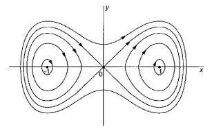
  Figure 2: The period annuli in the Duffing oscillator.

  In this example we study the so-called interior Duffing oscillator. Theorem 1.3 in [11] shows that at most two limit cycles bifurcate from either one of the interior period annuli.

  If we perform a translation to bring the center on the right half-plane to the origin, the Hamiltonian function of the unperturbed system becomes

  $$H(x,y)=A(x)+B(x)y^{2}\,\mbox{ with $A(x)=x^{2}+\frac{1}{4}x^{4}+x^{3}$ and $B(x)=\frac{1}{2}.$}$$

  The projection of the period annulus of this center is $\bigl{(}-1,\sqrt{2}-1\bigr{)}$ and $h_{0}=A(-1)=1/4.$

  From Theorem 2.1 in [11], it follows that the first non-identically zero Melnikov function is a linear combination of $\widetilde{I}_{i}(h)=\int_{\gamma_{h}}x^{i}ydx$ for $i=0,1,2.$ Thus, Theorem 1.3 in [11] will follow if we prove that $\bigl{\{}\widetilde{I}_{0},\widetilde{I}_{1},\widetilde{I}_{2}\bigr{\}}$ is an ECT-system. Additionally, this fact implies that there are values of the parameters for which exactly $0$, $1$ or $2$ limit cycles bifurcate from the period annulus. To this end we will apply Theorem B, but we note that in this case $m=1,$ $n=3$ and $s=1,$ so that the hypothesis $s>m(n-2)$ is not satisfied. This is easy to overcome because

  $$\widetilde{I}_{0}(h)=\int_{\gamma_{h}}ydx=\frac{1}{h}\int_{\gamma_{h}}\bigl{(}A(x)+B(x)y^{2}\bigr{)}ydx=\frac{1}{h}\int_{\gamma_{h}}A(x)ydx+\frac{1}{h}\int_{\gamma_{h}}B(x)y^{3}dx,$$

  and then, we apply Lemma 4.1 with $k=3$ and $F=A$ to the first integral above, to get

  $$\widetilde{I}_{0}(h)=\frac{1}{h}\int_{\gamma_{h}}\frac{x^{2}+2x+2}{12(x+1)^{2}}\,y^{3}dx+\frac{1}{h}\int_{\gamma_{h}}\frac{1}{2}\,y^{3}dx=\frac{1}{h}\int_{\gamma_{h}}f_{0}(x)y^{3}dx\,\mbox{ with }f_{0}(x)\!:=\frac{7x^{2}+14x+8}{12(x+1)^{2}}.$$

  (It is not possible to apply Lemma 4.1 directly to $\widetilde{I}_{0}$ because then we must take $F\equiv 1,$ and in this case $F/A^{\prime}$ is not analytic at $x=0.)$ Exactly in the same way we obtain

  $$\begin{array}[]{ll}\displaystyle\widetilde{I}_{1}(h)=\frac{1}{h}\int_{\gamma_{h}}f_{1}(x)y^{3}dx&\,\mbox{ with }\displaystyle f_{1}(x)\!:=\frac{x(8x^{2}+17x+10)}{12(x+1)^{2}},\\[15.0pt] \displaystyle\widetilde{I}_{2}(h)=\frac{1}{h}\int_{\gamma_{h}}f_{2}(x)y^{3}dx&\,\mbox{ with }\displaystyle f_{2}(x)\!:=\frac{x^{2}(9x^{2}+20x+12)}{12(x+1)^{2}}.\end{array}$$

  We set $I_{i}(h)=\int_{\gamma_{h}}f_{i}(x)y^{3}dx$ and it is clear that $\bigl{\{}\widetilde{I}_{0},\widetilde{I}_{1},\widetilde{I}_{2}\bigr{\}}$ is an ECT-system on $(0,h_{0})$ if and only if so it is $\{I_{0},I_{1},I_{2}\}.$ We can now apply Theorem B because $s=2$ and the condition $s>m(n-2)$ holds. Thus, setting

  $$\textstyle{\ell_{i}(x)=\left(\frac{f_{i}}{A^{\prime}}\right)\!(x)-\left(\frac{f_{i}}{A^{\prime}}\right)\!\bigl{(}\sigma(x)\bigr{)}},$$

  we have to check that $\{\ell_{0},\ell_{1},\ell_{2}\}$ is a CT-system on $\bigl{(}0,\sqrt{2}-1\bigr{)}.$ Here $\sigma$ is the involution associated to $A$ and we used that $B$ is constant. (In this example we can compute the involution explicitly but we do not use it because we want to show that it is not necessary to apply our result.) As a matter of fact we will show that $\{\ell_{0},\ell_{1},\ell_{2}\}$ is an ECT-system because a continuous Wronskian is easy to study. In order to compute the three Wronskians, we write $\ell_{i}(x)=L_{i}\bigl{(}x,\sigma(x)\bigr{)}$ with $L_{i}(x,z)=\bigl{(}\frac{f_{i}}{A^{\prime}}\bigr{)}(x)-\bigl{(}\frac{f_{i}}{A^{\prime}}\bigr{)}(z).$ Moreover, due to

  $$\textstyle{A(x)-A(z)=\frac{1}{4}(x-z)(x+2+z)(x^{2}+2x+2z+z^{2})},$$

  it turns out that $z=\sigma(x)$ is defined by means of $q(x,z)\!:=x^{2}+2x+2z+z^{2}=0.$ Accordingly, since $\sigma^{\prime}(x)=-\frac{x+1}{z+1},$ we have that $W[\mathbf{\ell_{i}}](x)=\omega_{i}\bigl{(}x,\sigma(x)\bigr{)}$ with $\omega_{i}(x,z)$ being a rational function for $i=1,2,3.$ The resultant with respect to $z$ between $q(x,z)$ and the numerator of $\omega_{3}(x,z)$ is $r_{3}(x)=64x^{16}(x+2)^{16}p_{3}(x)$ with

  $$p_{3}(x)= \,441\,{x}^{20}+8820\,{x}^{19}+79380\,{x}^{18}+423360\,{x}^{17}+1481685\,{x}^{16}+3555024\,{x}^{15}+5918640\,{x}^{14}$$

  $$+6740160\,{x}^{13}+4976155\,{x}^{12}+1881540\,{x}^{11}-892716\,{x}^{10}-3303200\,{x}^{9}-4779945\,{x}^{8}$$

  $$-3240840\,{x}^{7}+601960\,{x}^{6}+2523360\,{x}^{5}+1158080\,{x}^{4}-414400\,{x}^{3}-414400\,{x}^{2}+44800,$$

  and by applying Sturm’s Theorem we can assert that $p_{3}(x)\neq 0$ for all $x\in\bigl{(}0,\sqrt{2}-1\bigr{)}.$ Thus, $\omega_{3}(x,z)=0$ and $q(x,z)=0$ have no common roots, and this fact implies that $W[\mathbf{\ell_{3}}](x)\neq 0$ for all $x\in\bigl{(}0,\sqrt{2}-1\bigr{)}.$ The resultant with respect to $z$ between $q(x,z)$ and the numerator of $\omega_{2}(x,z)$ is $r_{2}(x)=32x^{7}(x+2)^{7}p_{2}(x)$ with

  $$p_{2}(x)= \,49\,{x}^{12}+588\,{x}^{11}+2940\,{x}^{10}+7840\,{x}^{9}+11650\,{x}^{8}+8528\,{x}^{7}$$

  $$+496\,{x}^{6}-3520\,{x}^{5}-1915\,{x}^{4}-620\,{x}^{3}-620\,{x}^{2}+360,$$

  and using Sturm’s Theorem it follows that $p_{2}$ does not vanish on $(0,\sqrt{2}-1).$ Exactly as before, this fact shows that $W[\mathbf{\ell_{2}}](x)\neq 0$ for all $x\in\bigl{(}0,\sqrt{2}-1\bigr{)}.$ Finally, the resultant with respect to $z$ between $q(x,z)$ and the numerator of $\omega_{1}(x,z)$ is

  $$r_{1}(x)=2\,{x}^{3}\left(x+2\right)^{3}\left(49\,{x}^{8}+392\,{x}^{7}+1176\,{x}^{6}+1568\,{x}^{5}+659\,{x}^{4}-500\,{x}^{3}-500\,{x}^{2}+80\right)$$

  and, thanks to Sturm’s Theorem again, we can assert that it does not vanish on $(0,\sqrt{2}-1).$ This proves that $W[\mathbf{\ell_{1}}](x)=\ell_{0}(x)\neq 0$ for all $x\in(0,\sqrt{2}-1).$ Consequently $\{\ell_{0},\ell_{1},\ell_{2}\}$ is an ECT-system on $(0,\sqrt{2}-1)$ and by applying Theorem B, $\{I_{0},I_{1},I_{2}\}$ is an ECT-system on $(0,1/4).$ Therefore, the first Melnikov function has at most two zeros counting multiplicities. $\square$

• Zhao, Liang and Lu study in [24] the system of planar differential equations

  $$\left\{\begin{array}[]{l}\dot{x}=2xy+\varepsilon\Bigl{(}\displaystyle\sum_{i+j\leqslant 2}a_{ij}(\varepsilon)x^{i}y^{j}\Bigr{)},\\[12.0pt] \dot{y}=6x-6x^{2}-y^{2}+\varepsilon\Bigl{(}\displaystyle\sum_{i+j\leqslant 2}b_{ij}(\varepsilon)x^{i}y^{j}\Bigr{)}.\end{array}\right.$$

  The unperturbed system (i.e., with $\varepsilon=0$) has a center at $(1,0)$ whose period annulus is bounded by a cuspidal loop and they prove (see Theorem 1.2 in [24]) that the maximum number of limit cycles emerging from its period annulus for $\varepsilon\approx 0$ is two.

  Our goal is to reobtain this result by applying Theorem B. To this end, we bring the center to the origin by means of a translation, so that the unperturbed system is Hamiltonian with

  $$H(x,y)=A(x)+B(x)y^{2},\,\mbox{ where $A(x)=x^{2}(3+2x)$ and $B(x)=x+1.$}$$

  The projection of the period annulus is now $(-1,1/2)$ and the energy level of the polycycle in its outer boundary is $h_{0}=A(-1)=1.$ By Theorem 3 in [16], the upper bound for the number of limit cycles is equal to the maximum number of zeros for $h\in(0,1),$ counted with multiplicities, of any non-trivial linear combination of

  $$\widetilde{I}_{i}(h)=\int_{\gamma_{h}}(x+1)^{i-1}ydx\,\mbox{ for $i=0,1,2.$}$$

  Accordingly, the result in [24] will follow once we show that $\bigl{\{}\widetilde{I}_{0},\widetilde{I}_{1},\widetilde{I}_{2}\bigr{\}}$ is an ECT-system on $(0,1).$ By applying Lemma 4.1, the same straightforward manipulation as before shows that $\widetilde{I}_{i}(h)=\frac{1}{18h}I_{i}(h)$ where

  $$I_{i}(h)=\int_{\gamma_{h}}f_{i}(x)y^{3}dx$$

  with

  $$f_{0}(x)=\frac{16x^{2}+35x+24}{(x+1)^{2}}\,,\ \mbox{ }f_{1}(x)=\frac{20x^{2}+41x+24}{x+1}\,\ \mbox{ and }\ f_{2}(x)=24x^{2}+47x+24.$$

  It is clear that $\bigl{\{}\widetilde{I}_{0},\widetilde{I}_{1},\widetilde{I}_{2}\bigr{\}}$ is an ECT-system on the interval $(0,1)$ if, and only if, so it is $\{I_{0},I_{1},I_{2}\}.$ On account of Theorem B, this will follow once we check that $\{\ell_{0},\ell_{1},\ell_{2}\}$ is an ECT-system on $(0,1/2),$ where $\ell_{i}=\mathscr{B}_{\sigma}\!\left(\frac{f_{i}}{A^{\prime}B^{3/2}}\right).$ Note that $A(x)-A(z)=(x-z)(2x^{2}+2zx+3x+2z^{2}+3z),$ so that $z=\sigma(x)$ is implicitly defined by means of $q(x,z)\!:=2x^{2}+2zx+3x+2z^{2}+3z=0.$ Thus

  $$\sigma^{\prime}(x)=\frac{dz}{dx}=-\frac{4x+2z+3}{4z+2x+3}.$$

  Taking this into account, some computations show that, for $i=1,2,3,$ $W[\,\mathbf{\ell_{i}}](x)=\omega_{i}\bigl{(}x,\sigma(x)\bigr{)}$ with $\omega_{i}(x,z)$ being a rational function of $u=\sqrt{x+1}$ and $v=\sqrt{z+1},$ say $R_{i}(u,v).$ Note that $x\longmapsto\sqrt{x+1}$ maps $(0,1/2)$ to $(1,\sqrt{3/2}).$ The resultant with respect to $v$ between the numerator of $R_{i}(u,v)$ and $q(u^{2}-1,v^{2}-1)$ is a polynomial $r_{i}(u)$ that, by applying Sturm’s Theorem, has no roots on $(1,\sqrt{3/2}).$ (For the sake of shortness we do not give here the expression of these polynomials.) Hence, it is proved that $W[\,\mathbf{\ell_{i}}]$ does not vanish on $(0,1/2)$ for $i=1,2,3.$ By Theorem B, this reasoning proves the mentioned result of Zhao, Liang and Lu. $\square$

• Peng studies in [21] the system of planar differential equations

  $$\left\{\begin{array}[]{l}\dot{x}=-y-3x^{2}-y^{2}+\varepsilon(\mu_{1}x+\mu_{2}xy),\\[5.0pt] \dot{y}=x(1-2y)+\varepsilon\mu_{3}x^{2}.\end{array}\right.$$

  The unperturbed system (i.e. when $\varepsilon=0$) has a center at the origin and the author proves (see Theorem A in [21]) that two is the maximal number of limit cycles which bifurcate from its period annulus for $\varepsilon\approx 0$ and that there are perturbations with exactly $0$, $1$ or $2$ limit cycles. To this end, he first shows that by means of the projective coordinate transformation $(x,y)\mapsto(\frac{y}{x+2},\frac{x}{2(x+2)})$ and a non-constant rescaling of time the above system reads for

  $$\left\{\begin{array}[]{l}\dot{x}=2(x+2)y+\varepsilon\mu_{3}(x+2)y^{2},\\[5.0pt] \dot{y}=-x-\frac{3}{4}x^{2}-y^{2}+\varepsilon\bigl{(}\mu_{1}(x+2)+\frac{\mu_{2}}{2}x+\mu_{3}y^{2}\bigr{)}.\end{array}\right.$$

  The unperturbed system is now Hamiltonian with a center at the origin whose period annulus is bounded by a saddle loop. We have written the transformations so as to directly apply Theorem B. The Hamiltonian function of the unperturbed system is

  $$H(x,y)=A(x)+B(x)y^{2}\,\mbox{ with $A(x)=\frac{1}{4}x^{2}(x+2)$ and $B(x)=x+2.$}$$

  The projection of the period annulus is $(-4/3,2/3)$ and the polycycle at its outer boundary has energy level $h_{0}=A(2/3)=8/27.$ It is very easy to show that the first Melnikov function is a linear combination of

  $$\widetilde{I}_{i}(h)=\int_{\gamma_{h}}(x+2)^{i}ydx\,\mbox{ for $i=0,1,2.$}$$

  Hence, the aforementioned result will follow once we check that $\bigl{\{}\widetilde{I}_{0},\widetilde{I}_{1},\widetilde{I}_{2}\}$ is an ECT-system on $(0,h_{0}).$ By using Lemma 4.1 exactly as before, $\widetilde{I}_{i}(h)=\frac{1}{h}I_{i}(h)$ where

  $$I_{i}(h)=\int_{\gamma_{h}}f_{i}(x)y^{3}dx$$

  with $f_{0}(x)=\frac{2(x+2)(15{x}^{2}+42x+32)}{3(3x+4)^{2}},$ $f_{1}(x)=\frac{4(x+2)^{2}(9{x}^{2}+23x+16)}{3(3x+4)^{2}}$ and $f_{2}(x)=\frac{2(x+2)^{3}(21{x}^{2}+50x+32)}{3(3x+4)^{2}}.$ Once again, $\bigl{\{}\widetilde{I}_{0},\widetilde{I}_{1},\widetilde{I}_{2}\bigr{\}}$ is an ECT-system on $(0,h_{0})$ if, and only if, so it is $\{I_{0},I_{1},I_{2}\}.$ The involution associated to $A$ is $z=\sigma(x)$ given by $q(x,z)\!:=x^{2}+xz+2x+z^{2}+2z=0$ because $A(x)-A(z)=\frac{1}{4}(x-z)q(x,z).$ Thus

  $$\sigma^{\prime}(x)=\frac{dz}{dx}=-\frac{z+2x+2}{x+2z+2}$$

  and, setting $\ell_{i}=\mathscr{B}_{\sigma}\!\left(\frac{f_{i}}{A^{\prime}B^{3/2}}\right),$ we have to verify that $W[\mathbf{\ell_{i}}]$ does not vanish on $(0,2/3)$ for $i=1,2,3.$ It can be shown that, for $i=1,2,3,$ $W[\mathbf{\ell_{i}}](x)=\omega_{i}\bigl{(}x,\sigma(x)\bigr{)}$ with $\omega_{i}(x,z)$ being a rational function of $u=\sqrt{x+2}$ and $v=\sqrt{z+2},$ say $R_{i}(u,v).$ We note that $x\longmapsto\sqrt{x+2}$ maps $(0,2/3)$ to $(\sqrt{2},\sqrt{8/3}).$ The resultant with respect to $v$ between the numerator of $R_{i}(u,v)$ and $q(u^{2}-2,v^{2}-2)$ is a polynomial $r_{i}(u)$ that, by applying Sturm’s Theorem, has no roots on $(\sqrt{2},\sqrt{8/3}).$ Therefore, $W[\,\mathbf{\ell_{i}}]$ does not vanish on $(0,2/3)$ for $i=1,2,3.$ By Theorem B, we have proved the result of Peng in [21]. $\square$

4.1 Results on the program of Gautier, Gavrilov and Iliev

Our last examples of application come from the paper of Gautier, Gavrilov and Iliev [8], where a program for finding the cyclicity of the period annuli of quadratic systems with centers of genus one is presented. They give a list of the essential perturbations of these centers (i.e., the one-parameter perturbations that produce the maximal number of limit cycles), together with the corresponding generating function of limit cycles (i.e., the Poincaré-Pontryagin-Melnikov function). Since some cases have been already solved in the literature about the problem, this list includes only the open cases, a total of 26. They conjecture that the cyclicity of these period annuli is two, except for some particular cases in which it is three (cf. Conjecture 1 in page 12 and Conjecture 2 in page 17). In their Theorem 3, two quadratic reversible systems with a center are considered, denoted by (r11) and (r18) in the list, and they show that, in both cases, the upper bound of the number of limit cycles produced by the period annulus under quadratic perturbations is equal to two. We are going to reobtain this result for the case (r11) by using our criterion. Moreover, we prove their conjecture in four new cases in their list, namely (r7-r14), (r15), (r17) and (rlv3). In fact, Theorem B is likely to be applied in many of their cases but we have only been able to directly show that the functions on the integrand satisfy the Chebyshev condition in the five mentioned cases. We remark that our criterion gives a sufficient condition for the Abelian integrals to be an ECT-system.

Case (r11) We translate the center to the origin, so that the first integral of the unperturbed system is

$$H(x,y)=A(x)+B(x)y^{2}\,\mbox{ with $A(x)=\frac{x^{2}(x+3)}{6(x+1)^{3}}$ and $B(x)=\frac{1}{2(x+1)^{3}}.$}$$

They show that the cyclicity of the period annulus under quadratic perturbations is two. This will follow once we show that $\bigl{\{}\widetilde{I}_{0},\widetilde{I}_{1},\widetilde{I}_{2}\bigr{\}}$ is an ECT-system on $(0,1/6),$ where

$$\widetilde{I}_{i}(h)=\int_{\gamma_{h}}(x+1)^{i-2}ydx.$$

The projection of the period annulus of the center at the origin is $(-1/3,+\infty).$ By applying Lemma 4.1 once again, $\widetilde{I}_{i}(h)=\frac{1}{36h}I_{i}(h)$ where $I_{i}(h)=\int_{\gamma_{h}}f_{i}(x)y^{3}dx$ with

$$f_{0}(x)=\frac{5{x}^{2}+13x+24}{(x+1)^{5}},\;f_{1}(x)=\frac{7{x}^{2}+19x+24}{(x+1)^{4}}\,\mbox{ and }f_{2}(x)=\frac{9{x}^{2}+25x+24}{(x+1)^{3}}.$$

It is clear then that it suffices to show that $\{I_{0},I_{1},I_{2}\}$ is an ECT-system on $(0,1/6).$ With this aim in view, let us note that $A(x)-A(z)=\frac{(x-z)q(x,z)}{6(x+1)^{3}(z+1)^{3}}$ with $q(x,z)\!:=3x^{2}z+x^{2}+10xz+3x+3xz^{2}+z^{2}+3z,$ so that the involution $z=\sigma(x)$ associated to $A$ satisfies $q\bigl{(}x,\sigma(x)\bigr{)}=0.$ Taking this into account, we get that

$$\sigma^{\prime}(x)=\frac{dz}{dx}=-\frac{x(z+1)^{4}}{z(x+1)^{4}}.$$

As before we must compute the Wronskians $W[\,\mathbf{\ell_{i}}](x)$ for $i=1,2,3,$ where $\ell_{i}=\mathscr{B}_{\sigma}\!\left(\frac{f_{i}}{A^{\prime}B^{3/2}}\right),$ and then show that they do not vanish for $x\in(0,+\infty).$ In this case $W[\mathbf{\ell_{i}}](x)=\omega_{i}\bigl{(}x,\sigma(x)\bigr{)}$ with $\omega_{i}(x,z)$ being a rational function of $u=\sqrt{x+1}$ and $v=\sqrt{z+1},$ say $R_{i}(u,v).$ The resultant with respect to $v$ between the numerator of $R_{i}(u,v)$ and $q(u^{2}-1,v^{2}-1)$ is a polynomial $r_{i}(u).$ Since the mapping $x\longmapsto\sqrt{x+1}$ sends $(0,+\infty)$ to $(1,+\infty),$ the result will follow once we show that these polynomials $r_{i}(u)$ do not vanish on $(1,+\infty)$. This latter fact is deduced from the application of Sturm’s Theorem.$\square$

Let us mention that we have studied the case (r18) as well (the other case that contemplates Theorem 3 in [8]), but it seems that it cannot be solved by using the criterion given by our Theorem B. Of course, the success in the application of this criterion depends on the particular problem studied, but we want to stress that, when it works, it enables to extremely simplify the solution. For instance, the proof of Theorem 3 takes eight pages of highly nontrivial arguments. From now on, for the sake of brevity in the exposition, we omit many of the explanations on the way to apply our criterion since they are a verbatim repetition of the previous examples.

Cases (r7-r14) and (r15) The first integral is shared by the two cases and, after we translate the center at the origin, it reads for

$$H(x,y)=\frac{y^{2}}{2}+\frac{x^{2}(3x^{2}+8x+6)}{12}.$$

The cyclicity of the period annulus, whose projection on the $x$-axis is the interval $(-1,1/3)$, is two if we prove that $\bigl{\{}\widetilde{I}_{0},\widetilde{I}_{1},\widetilde{I}_{2}\bigr{\}}$ is an ECT-system for $h\in(0,1/12),$ where

$$\begin{array}[]{l}\displaystyle\widetilde{I}_{i}(h)\,=\,\int_{\gamma_{h}}(x+1)^{i-2}ydx\ \ \mbox{for the case (r7-r14)},\vspace{0.2cm}\\ \displaystyle\widetilde{I}_{i}(h)\,=\,\int_{\gamma_{h}}(x+1)^{i-4}ydx\ \ \mbox{for the case (r15)}.\end{array}$$

We apply Lemma 4.1 to the Abelian integrals given by $I_{i}(h)=h\,\widetilde{I}_{i}(h)$ in order to write them in the form $I_{i}(h)=\int_{\gamma_{h}}f_{i}(x)y^{3}dx$. We have that:

$$\begin{array}[]{l}\displaystyle\int_{\gamma_{h}}H(x,y)ydx\,=\,\int_{\gamma_{h}}\frac{21x^{3}+63x^{2}+64x+24}{36(x+1)^{3}}\,y^{3}dx,\\[10.0pt] \displaystyle\int_{\gamma_{h}}H(x,y)\,\frac{ydx}{x+1}=\int_{\gamma_{h}}\frac{(2x+3)(9x^{2}+14x+8)}{36(x+1)^{4}}\,y^{3}dx,\\[10.0pt] \displaystyle\int_{\gamma_{h}}H(x,y)\,\frac{ydx}{(x+1)^{2}}=\int_{\gamma_{h}}\frac{15x^{3}+47x^{2}+52x+24}{36(x+1)^{5}}\,y^{3}dx,\\[10.0pt] \displaystyle\int_{\gamma_{h}}H(x,y)\,\frac{ydx}{(x+1)^{3}}=\int_{\gamma_{h}}\frac{12x^{3}+39x^{2}+46x+24}{36(x+1)^{6}}\,y^{3}dx,\\[10.0pt] \displaystyle\int_{\gamma_{h}}H(x,y)\,\frac{ydx}{(x+1)^{4}}=\int_{\gamma_{h}}\frac{9x^{3}+31x^{2}+40x+24}{36(x+1)^{7}}\,y^{3}dx.\end{array}$$

Some computations show that the involution $\sigma$ defined by $A(x)\!:=H(x,0)$ satisfies $q\bigl{(}x,\sigma(x)\bigr{)}=0$ with $q(x,z)\!:=3z^{3}+3xz^{2}+8z^{2}+3x^{2}z+8xz+6z+3x^{3}+8x^{2}+6x$. We use resultants and Sturm’s Theorem in order to check that the corresponding Wronskians have no zeros on the interval $(0,1/3)$.$\square$

Case (r17) Once the center is translated to the origin, the first integral reads for

$$H(x,y)=\frac{y^{2}}{2}+\frac{(2x+3)x^{2}}{6}.$$

Setting $\widetilde{I}_{i}(h)=\int_{\gamma_{h}}(x+1)^{i-3}ydx,$ the cyclicity of its period annulus is two if we prove that $\bigl{\{}\widetilde{I}_{0},\widetilde{I}_{1},\widetilde{I}_{2}\bigr{\}}$ is an ECT-system on $(0,1/6).$ By Lemma 4.1, we have that $\widetilde{I}_{i}(h)=\frac{1}{18h}\int_{\gamma_{h}}f_{i}(x)y^{3}dx,$ with

$$f_{0}(x)=\frac{5x^{2}+13x+12}{(x+1)^{5}},\ f_{1}(x)=\frac{7x^{2}+16x+12}{(x+1)^{4}}\ \mbox{and}\ f_{2}(x)=\frac{9x^{2}+19x+12}{(x+1)^{3}}.$$

In this case, the involution $\sigma$ defined by $A(x)\!:=H(x,0)$ satisfies $q\bigl{(}x,\sigma(x)\bigr{)}=0$ where $q(x,z)\!:=2z^{2}+2xz+3z+2x^{2}+3x$. The projection of the period annulus on the $x$-axis is $(-1,1/2)$ and, thus, we are done if we show that the functions $\ell_{i}=\mathscr{B}_{\sigma}\!\left(\frac{f_{i}}{A^{\prime}B^{3/2}}\right)$ form an ECT-system in $(0,1/2)$. Once again, the involution can be explicitly written, but we prefer to use resultants and Sturm’s Theorem because it provides an algebraic procedure to check that the Wronskians $W[\,\mathbf{\ell_{i}}]$ do not vanish on $(0,1/2)$ for $i=1,2,3.$ The proof of this fact is omitted for the sake of shortness.$\square$

Case (rlv3) After the center is translated to the origin, the first integral becomes

$$H(x,y)=x^{2}(2-x^{2})+\frac{1}{2}(1+x)^{2}y^{2}.$$

Since $A(x)\!:=H(x,0)$ is an even function, we have that $\sigma(x)=-x$ and this simplifies a lot the computations. The projection of the period annulus on the $x$-axis is $(-1,1)$. In order to prove that its cyclicity under quadratic perturbations is two, we are lead to show that $\bigl{\{}I_{0},I_{1},I_{2}\bigr{\}}$ form an ECT-system for $h\in(0,1),$ where $I_{i}(h)=\int_{\gamma_{h}}f_{i}(x)y^{3}dx$ with $f_{0}(x)=\frac{(5x^{4}-2x^{3}-9x^{2}+4x+8)(x+1)}{2(x-1)^{4}},$ $f_{1}(x)=\frac{(7x^{4}-13x^{2}+8)(x+1)}{(x-1)^{2}}$ and $f_{2}(x)=\frac{6x^{4}+x^{3}-11x^{2}-2x+8}{(x-1)^{2}}.$ To this end, by applying Theorem B and taking $\sigma(x)=-x$ into account, it suffices to show that the functions

$$\ell_{0}(x)=\frac{5x^{6}-8x^{4}+7x^{2}+8}{2x(x-1)^{5}(x+1)^{5}},\ \ \ell_{1}(x)=\frac{7x^{4}-13x^{2}+8}{x(x-1)^{3}(x+1)^{3}}\ \mbox{ and }\ \ell_{2}(x)=\frac{5x^{4}-9x^{2}+8}{x(x-1)^{4}(x+1)^{4}}$$

form an ECT-system on $(0,1).$ It is easy to see that $\ell_{2}$ does not vanish on $(0,1)$. The Wronskian associated to $\ell_{1}$ and $\ell_{2}$ is the rational function

$$W[\ell_{1},\ell_{2}](x)=\frac{96-240x^{2}+243x^{4}-126x^{6}+35x^{8}}{18x(x-1)^{8}(x+1)^{8}},$$

which has no zero on $(0,1)$ by virtue of Sturm’s Theorem. Finally

$$W[\ell_{0},\ell_{1},\ell_{2}](x)=\frac{2(512-1632x^{2}+2200x^{4}-1617x^{6}+693x^{8}-175x^{10}+35x^{12})}{9(x-1)^{15}(x+1)^{15}},$$

which neither vanishes on $(0,1)$, again by using Sturm’s Theorem. As desired, this shows that $(\ell_{2},\ell_{1},\ell_{0})$ is an ECT-system on $(0,1).$$\square$

5 Appendix

5.1 Resultant of two polynomials

Given two polynomials $p,q\in\mathbb{C}[x,y],$ say

$$p(x)=a_{0}x^{m}+a_{1}x^{m-1}+\ldots+a_{m},\,\mbox{ with $a_{0}\neq 0,$}$$

$$q(x)=b_{0}x^{n}+b_{1}x^{n-1}+\ldots+b_{n},\,\mbox{ with $b_{0}\neq 0,$}$$

where $a_{i},b_{i}\in\mathbb{C}[y]$, the resultant of $p$ and $q$ with respect to $x$, denoted by $\mbox{Res}(p,q,x)$ is the $(m+n)\!\times\!(m+n)$ determinant

$$\mbox{Res}(p,q,x)\,=\,\det\left(\begin{array}[]{cccccccc}a_{0}&&&&b_{0}&&&\\ a_{1}&a_{0}&&&b_{1}&b_{0}&&\\ a_{2}&a_{1}&\ddots&&b_{2}&b_{1}&\ddots&\\ \vdots&a_{2}&\ddots&a_{0}&\vdots&\ddots&&b_{0}\\ a_{m}&\vdots&\ddots&a_{1}&b_{n}&\vdots&\ddots&b_{1}\\ &a_{m}&&a_{2}&&b_{n}&&b_{2}\\ &&\ddots&\vdots&&&\ddots&\vdots\\ &&&a_{m}&&&&b_{n}\\ \end{array}\right)$$

where the blank spaces are filled with zeros. The three basic properties of the resultant are:

1. $\mbox{Res}(p,q,x)$ is an integer polynomial in the coefficients of $p$ and $q$.

2. $\mbox{Res}(p,q,x)=0$ if, and only if, $p$ and $q$ have a nontrivial common factor in $\mathbb{C}[x,y]$.

3. There are polynomials $A,B\in\mathbb{C}[x,y]$ such that $Ap+Bq=\mbox{Res}(p,q,x).$ Moreover the coefficients of $A$ and $B$ are integer polynomials in the coefficients of $p$ and $q$.

Resultants can be used to eliminate variables from systems of polynomial equations. As an example, let us suppose that we want to study the following system of two polynomial equations with two variables:

$$\left\{\begin{array}[]{l}xy-1=0,\\[2.0pt] x^{2}+y^{2}-4=0.\end{array}\right.$$

Here we have two variables to work with, but if we regard $p(x,y)\!:=xy-1$ and $q(x,y)\!:=x^{2}+y^{2}-4$ as polynomials in $x$ whose coefficients are polynomials in $y,$ we can compute the resultant with respect to $x$ to obtain $\mbox{Res}(p,q,x)=y^{4}-4y^{2}+1.$ By the third property above, there are polynomials $A,B\in\mathbb{C}[x,y]$ such that $A(x,y)p(x,y)+B(x,y)q(x,y)=y^{4}-4y^{2}+1.$ Accordingly, $y^{4}-4y^{2}+1$ vanishes at any common solution of $p=q=0.$ Thus, we can solve $y^{4}-4y^{2}+1=0$ and find the $y$-coordinates of these solutions.

5.2 Sturm’s Theorem

A sequence $\{f_{0},f_{1},\ldots,f_{m}\}$ of continuous real functions on $[a,b]$ is called a Sturm’s sequence for $f=f_{0}$ on $[a,b]$ if the following is verified:

1. $f_{0}$ is differentiable on $[a,b].$

2. $f_{m}$ does not vanish on $[a,b].$

3. If $f(x_{0})=0$ with $x_{0}\in[a,b]$ then $f_{1}(x_{0})f_{0}^{\prime}(x_{0})>0.$

4. If $f_{i}(x_{0})=0$ with $x_{0}\in[a,b]$ then $f_{i+1}(x_{0})f_{i-1}(x_{0})<0.$

• Let $\{f_{0},f_{1},\ldots,f_{m}\}$ be a Sturm’s sequence for $f=f_{0}$ on $[a,b]$ with $f(a)f(b)\neq 0.$ Then the number of roots of $f$ on $(a,b)$ is equal to $V(a)-V(b),$ where $V(c)$ is the number of changes of sign in the sequence $\{f_{0}(c),f_{1}(c),\ldots,f_{m}(c)\}.$

There is a simple procedure to construct a Sturm’s sequence in case that $f$ is polynomial. Indeed, if $p(x)$ is a polynomial of degree $n$, we define the sequence $\{p_{0},p_{1},\ldots,p_{m}\}$ with $m\leqslant n$ in the following way. We set $p_{0}=p,$ $p_{1}=p^{\prime}$ and

$$p_{i-1}(x)=q_{i}(x)p_{i}(x)-p_{i+1}(x),\,\mbox{ for $i=1,2,\ldots,m-1,$}$$

$$p_{m-1}(x)=q_{m}(x)p_{m}(x),$$

where $q_{i}(x)$ and $p_{i+1}(x)$ are the quotient and the remainder (the latter with the sign changed) of the division of $p_{i-1}(x)$ by $p_{i}(x)$, respectively. The construction of this sequence ends when the remainder is zero, i.e., $p_{m+1}=0.$ In this case, since this is essentially Euclides’ algorithm, $p_{m}$ is the greatest common divisor of $p_{0}$ and $p_{1}.$ If all the zeros of $p$ are simple then $p_{m}$ does not vanish and it is easy to show that $\{p_{0},p_{1},\ldots,p_{m}\}$ is a Sturm’s sequence for $p$ on any interval. If $p$ has zeros with multiplicity then $p_{m}$ vanishes. Since $p_{m}$ divides $p_{0}$ and $p_{1},$ it also divides $p_{i}$ for $i=2,3,\ldots,m$. In this case, we set $\bar{p}_{i}=p_{i}/p_{m}$ and it follows that $\{\bar{p}_{0},\bar{p}_{1},\ldots,\bar{p}_{m}\}$ is a Sturm’s sequence for $p$ on any interval.

References

- [1] V.I. Arnold, “Arnold’s problems”, Springer-Verlag, Berlin, 2004.
- [2] F. Dumortier and Chengzhi Li, Perturbations from an elliptic Hamiltonian of degree four. I. Saddle loop and two saddle cycle, J. Differential Equations 176 (2001) 114–157.
- [3] F. Dumortier and Chengzhi Li, Perturbations from an elliptic Hamiltonian of degree four. II. Cuspidal loop, J. Differential Equations 175 (2001) 209–243.
- [4] F. Dumortier, Chengzhi Li and Zifen Zhang, Unfolding of a quadratic integrable system with two centers and two unbounded heteroclinic loops, J. Differential Equations 139 (1997) 146–193.
- [5] F. Dumortier and R. Roussarie, Abelian integrals and limit cycles, J. Differential Equations 227 (2006) 116–165.
- [6] Maoan Han, Existence of at most 1, 2, or 3 zeros of a Melnikov function and limit cycles, J. Differential Equations 170 (2001) 325–343.
- [7] E. Horozov and I. Iliev, On the number of limit cycles in perturbations of quadratic Hamiltonian systems, Proc. London Math. Soc. 69 (1994) 198–224.
- [8] S. Gautier, L. Gavrilov and I. Iliev, Perturbations of quadratic centers of genus one, preprint (2008) arXiv:0705.1609v2 [math.DS].
- [9] A. Gasull, Weigu Li, J. Llibre and Zhifen Zhang, Chebyshev property of complete elliptic integrals and its application to Abelian integrals, Pacific J. Math. 202 (2002) 341–361.
- [10] F. Girard, Une propriété de Chebychev pour certaines intégrales abéliennes généralisées, C. R. Acad. Sci. Paris Sér. I Math. 326 (1998) 471–476.
- [11] I. Iliev and L. Perko, Higher oder bifurcations of limit cycles, J. Differential Equations 154 (1999) 339–363.
- [12] L. Gavrilov, The infinitesimal 16th Hilbert problem in the quadratic case, Invent. Math. 143 (2001) 449–497.
- [13] L. Gavrilov and I. Iliev, Bifurcations of limit cycles from infinity in quadratic systems, Canad. J. Math. 54 (2002) 1038–1064.
- [14] L. Gavrilov and I. Iliev, Two-dimensional Fuchsian systems and the Chebyshev property, J. Differential Equations 191 (2003) 105–120.
- [15] D. Hilbert, Mathematische Problem lecture, Second Internat. Congress Math. Paris 1900, Nachr. Ges. Wiss. Göttingen Math.-Phys. Kl. 1900, 253–297.
- [16] I. Iliev, Perturbations of quadratic centers, Bull. Sci. Math. 122 (1998) 107–161.
- [17] Yu. Ilyashenko, Centennial history of Hilbert’s 16th problem, Bull. Amer. Math. Soc. (N.S.) 39 (2002) 301–354.
- [18] S. Karlin and W. Studden, “Tchebycheff systems: with applications in analysis and statistics”, Interscience Publishers, 1966.
- [19] Chengzhi Li and Zifen Zhang, A criterion for determining the monotonicity of the ratio of two Abelian integrals, J. Differential Equations 127 (1996) 407- 424.
- [20] Jibin Li, Hilbert’s 16th problem and bifurcations of planar polynomial vector fields. Internat. J. Bifur. Chaos Appl. Sci. Engrg. 13 (2003) 47–106.
- [21] Lin Ping Peng, Unfolding of a quadratic integrable system with a homoclinic loop, Acta Mathematica Sinica 18 (2002) 737 -754.
- [22] P. Mardešić, “Chebyshev systems and the versal unfolding of the cusp of order ”, Travaux en cours, vol. 57, Hermann, Paris, 1998.
- [23] G. Petrov, The Chebyshev property of elliptic integrals, Funct. Anal. Appl. 22 (1988) 72–73.
- [24] Yulin Zhao, Zhaojun Liang and Gang Lu, The cyclicity of the period annulus of the quadratic Hamiltonian systems with non-Morsean point, J. Differential Equations 162 (2000) 199–223.