Electromagnetic Circuits

Abstract

The electromagnetic analog of an elastic spring-mass network is constructed. These electromagnetic circuits offer the promise of manipulating electromagnetic fields in new ways, and linear electrical circuits correspond to a subclass of them. They consist of thin triangular magnetic components joined at the edges by cylindrical dielectric components. (There are also dual electromagnetic circuits consisting of thin triangular dielectric components joined at the edges by cylindrical magnetic components.) Some of the edges can be terminal edges to which electric fields are applied. The response is measured in terms of the real or virtual free currents that are associated with the terminal edges. The relation between the terminal electric fields and the terminal free currents is governed by a symmetric complex matrix ${\bf W}$. In the case where all the terminal edges are disjoint, and the frequency is fixed, a complete characterization is obtained of all possible response matrices ${\bf W}$ both in the lossless and lossy cases. This is done by introducing a subclass of electromagnetic circuits, called electromagnetic ladder networks. It is shown that an electromagnetic ladder network, structured as a cubic network, can have a macroscopic electromagnetic continuum response which is non-Maxwellian, and novel.

Keywords: Electromagnetism, Circuits, Networks, Metamaterials

1 Introduction

In this paper we introduce a new type of electrical circuit, called an electromagnetic circuit, which has the potential at a fixed frequency for providing new and easily analyzable ways of manipulating electromagnetic fields beyond those provided by electrical circuits, photonic circuits, optical lenses, waveguides, photonic crystals, and transformation optics. To construct the electromagnetic circuit we draw upon analogs between electromagnetism, elastodynamics and acoustics. Analogs between electromagnetism and elastodynamics have a long history [see, e.g. ?) and references therein] and can be understood from the viewpoint of differential geometry ([Oziewicz (1994]). It is easy to see the connection from the underlying partial differential equations when they are written in a form which emphasizes the similarity. Considering for simplicity a locally isotropic medium, Maxwell’s equations at fixed frequency $\omega$ take the form

$${\bf D}=\varepsilon{\bf E},\quad{\bf B}=\mu{\bf H},\quad\nabla\times{\bf E}=i\omega{\bf B},\quad\nabla\times{\bf H}={\bf j}-i\omega{\bf D},$$ (1.1)

where ${\bf D}({\bf x})$, ${\bf E}({\bf x})$, ${\bf B}({\bf x})$, ${\bf H}({\bf x})$, and ${\bf j}({\bf x})$ are the complex electric displacement field, electric field, magnetic induction, magnetic field, and free current (the physical fields are the real parts of $e^{-i\omega t}{\bf D}$, $e^{-i\omega t}{\bf E}$, $e^{-i\omega t}{\bf B}$, $e^{-i\omega t}{\bf H}$, and $e^{-i\omega t}{\bf j}$ where $t$ is time) and $\varepsilon({\bf x},\omega)$ and $\mu({\bf x},\omega)$ are the complex electric permittivity and complex magnetic permeability. Here the free current ${\bf j}({\bf x})$ may represent a single frequency component of a time varying ion beam current, or a time varying current generated by an electrochemical potential. It does not include conduction currents $\sigma{\bf E}$, where $\sigma$ is the conductivity, that instead are included in the term ${\bf D}=\varepsilon{\bf E}$, through the imaginary part of $\varepsilon({\bf x},\omega)$. (It is difficult, if not impossible, to distinguish oscillating displacement currents from oscillating conduction currents.) The elimination of ${\bf D}$, ${\bf B}$ and ${\bf H}$ leads to the form ([Milton, Briane, and Willis (2006]),

$$\frac{\partial}{\partial x_{p}}\left(C_{pqrs}\frac{\partial E_{s}}{\partial x_{r}}\right)+i\omega j_{q}=-\omega^{2}\varepsilon E_{q},$$ (1.2)

where

$$C_{pqrs}=e_{pqm}e_{rsm}/\mu,$$ (1.3)

and $e_{pqm}=1$ $(-1)$ if $(p,q,m)$ is an even (odd) permutation of (1,2,3) and is zero otherwise]. This is clearly similar to the form of the equations of continuum elastodynamics

$$\frac{\partial}{\partial x_{p}}\left(C_{pqrs}\frac{\partial u_{s}}{\partial x_{r}}\right)+f_{q}=-\omega^{2}\rho u_{q},$$ (1.4)

in which ${\bf u}({\bf x})$ and ${\bf f}({\bf x})$ are the complex displacement field, and body force (the physical fields are $\widetilde{{\bf u}}=(e^{-i\omega t}{\bf u})^{\prime}$ and $\widetilde{{\bf f}}=(e^{-i\omega t}{\bf f})^{\prime}$ where the prime denotes the real part) and ${\bf C}({\bf x},\omega)$ is the complex elasticity tensor (incorporating viscosity terms through its imaginary part) and $\rho({\bf x},\omega)$ is the density [which, when it is the effective density tensor of an isotropic composite material can be complex and has the same properties as a function of $\omega$ as $\varepsilon({\bf x},\omega)$: see ?) and references therein.] At low frequencies, one often has the approximation that ${\bf C}({\bf x},\omega)\approx{\bf C}^{\prime}({\bf x})-i\omega\mbox{\boldmath${\nu}$}({\bf x})$ where ${\bf C}^{\prime}({\bf x})$ is the real component of the elasticity tensor, and $\mbox{\boldmath${\nu}$}({\bf x})$ is the viscosity tensor, incorporating both bulk and shear viscosities. Then, upon introducing the velocity $\widetilde{v}={\partial\widetilde{u}}/{\partial t}$, (1.4) reduces to

$$\frac{\partial}{\partial x_{q}}(C^{\prime}_{pqrs}\frac{\partial\widetilde{u}_{s}}{\partial x_{r}}+\nu_{pqrs}\frac{\partial\widetilde{v}_{s}}{\partial x_{r}})+\widetilde{f}_{p}=\rho\frac{\partial\tilde{v}_{p}}{\partial t}$$ (1.5)

which may be more familiar to readers acquainted with the Kelvin-Voigt model of viscoelasticity.

As these analogies have been known for a long time it is rather amazing that no electromagnetic analog of a spring network with masses at the nodes has been constructed. Our electromagnetic circuits are this analog. In elastic networks, as modeled by the continuum construction of figure 1, the density is concentrated at the nodes, while the elasticity is concentrated along the edges. Everything is surrounded by void with ${\bf C}=0$ and $\mbox{\boldmath${\rho}$}=0$.

Figure 1: Sketch of a two-terminal discrete elastic network, where the terminal nodes are represented by the black circles, and the three internal nodes are represented by the white circles. In the idealized model these nodes have some mass and are infinitely stiff. They are are attached by connecting rods (which act as springs) having no mass and non-zero stiffness. Ideally the nodes should have infinitely small diameter and the connecting rods should be infinitely thin, although in practice one then has to worry about buckling which is a non-linear effect.

Besides the interest of electromagnetic circuits for providing a new way of manipulating electromagnetic fields there is also a fundamental reason for studying them. It is becoming increasingly clear that the usual continuum equations of physics do not apply to composite materials built from high contrast constituents and having exotic microstructures. Thus, one can obtain materials with macroscopic non-Ohmic, possibly non-local, conducting behavior, even though they conform to Ohm’s law at the microscale ([Khruslov (1978]; [Briane (1998]; [Briane and Mazliak (1998]; [Briane (2002], [Camar-Eddine and Seppecher (2002]; [Cherednichenko, Smyshlyaev, and Zhikov (2006]), materials with a macroscopic higher order gradient or non-local elastic response even though they are governed by usual linear elasticity equations at the microscale ([Pideri and Seppecher (1997]; [Bouchitté and Bellieud (2002]; [Alibert, dell’Isola, and Seppecher (2003]; [Camar-Eddine and Seppecher (2003]), materials with macroscopic behavior outside that of continuum elastodynamics even though they are governed by continuum elastodynamics at the microscale ([Milton (2007]), and materials with non-Maxwellian macroscopic electromagnetic behavior ([Shin, Shen, and Fan (2007]), even though they conform to Maxwell’s equations at the microscale [see also ?) where other non-Maxwellian macroscopic equations are proposed].

One would really like to be able to characterize the possible macroscopic continuum equations that govern the behavior of materials, including materials with exotic microstructures. A program for doing this was developed by Camar-Eddine and Seppecher (?, ?), and successfully applied to the conductivity and elastic equations in the three-dimensional static case, assuming the macroscopic behavior was governed by a single potential or displacement field. The program, in essence, consists of four steps: first to show that discrete networks can be modeled by a continuum construction; second to characterize all possible responses of discrete networks allowing for part of the network to be hidden; third to find the possible continuum limits of these discrete networks; and fourth to show that these possible continuum behaviors is all that there can be, even when one allows for other, non-network based, microstructures. For the dynamic case, at fixed frequency, a complete characterization has been obtained of the possible response matrices of multiterminal electrical, acoustic, and elastodynamic networks, both in two and three dimensions, thus meeting the second goal of the program in these cases ([Milton and Seppecher (2008]). For Maxwell’s equations at fixed frequency our electromagnetic circuits accomplish, in a formal way, the first goal of the program, and we also make progress towards the second goal. At this time it is unclear if our electromagnetic circuits are sufficiently rich in construction that their continuum limits can model the macroscopic behavior of all other, non-network based, microstructures, and in particular the question remains open as to whether the Maxwell equations themselves can be recovered as a continuum behavior of our electromagnetic circuits. It seems clear, however, that many non-Maxwellian continuum behaviors can be achieved (see the concluding paragraph of the paper).

We emphasize that, besides similarities, there are also important differences between Maxwell’s equations and the elasticity equations. For Maxwell’s equations the null space of ${\bf C}$ contains all symmetric matrices, while for elasticity the null space of ${\bf C}$ contains antisymmetric matrices, which is a space of lower dimension. This manifests itself in the different boundary conditions: at an interface ${\bf u}$ is required to be continuous, while only the tangential component of ${\bf E}$ is required to be continuous. In this respect Maxwell’s equations have some similarity with the acoustic equations, which (see (2.5)) take also a form analogous to (1.2) or (1.4), with

$$C_{pqrs}=\kappa\delta_{pq}\delta_{rs},$$ (1.6)

and the null space of ${\bf C}$ contains all matrices which have zero trace, and only the normal component of ${\bf u}$ is required to be continuous at an interface.

There are also linguistic differences when one discusses elasticity compared to electromagnetism. When one wants to study equation (1.2) in a bounded domain, boundary conditions are needed. A natural condition is to fix the value of ${\bf n}\cdot{\bf C}\partial{\bf E}/\partial{\bf x}$ where ${\bf n}$ is the external unit normal to the boundary of the domain. The analog boundary condition in the elastodynamic case is well known and called the surface force ${\bf F}$ applied to the medium. Thus we will call the applied surface free current the value of $(i\omega)^{-1}{\bf n}\cdot{\bf C}\partial{\bf E}/\partial{\bf x}$ on the boundary and denote it ${\bf J}$. (The additional factor of $(i\omega)^{-1}$ is introduced because $i\omega{\bf j}$ in (1.2) plays the role of ${\bf f}$ in (1.4).) This is not a usual way of speaking in the electromagnetic framework as the value of $(i\omega)^{-1}{\bf n}\cdot{\bf C}\partial{\bf E}/\partial{\bf x}$ is nothing else than the tangential part of the magnetic field ${\bf H}$ at the boundary. The interest of such a vocabulary appears later.

When one wants to study equation (1.2) in a domain $\Omega$ which is divided in two subdomains $\Omega_{1}$, $\Omega_{2}$, one has to write jump conditions on the dividing surface. This condition is the continuity of the tangential part of ${\bf H}$ (the analog of which is the continuity of the normal part of the stress in elastodynamic framework). Alternatively one says in the elastodynamics framework that $\Omega_{2}$ exerts on $\Omega_{1}$ a surface force ${\bf F}$ while $\Omega_{1}$ exerts on $\Omega_{2}$ the opposite surface force $-{\bf F}$. This action-reaction law makes the link with the separate study of both subdomains as it fixes the needed boundary conditions for these studies.

In a similar way we can say that $\Omega_{2}$ exerts on $\Omega_{1}$ a surface free current ${\bf J}$ while $\Omega_{1}$ exerts on $\Omega_{2}$ the opposite surface free current $-{\bf J}$. This way of thinking needs some practice to become natural and the reader should be aware that this formulation does not mean, in any way, that there exist actual free currents in the material (just like action-reaction law does not imply the existence of actual surface forces inside the domain). However the surface force ${\bf F}$ that $\Omega_{2}$ exerts on $\Omega_{1}$ has an equivalent effect on $\Omega_{1}$ as a body force ${\bf f}$ concentrated at the boundary replacing the stress field in $\Omega_{2}$, and similarly the applied surface free current ${\bf J}$ that $\Omega_{2}$ exerts on $\Omega_{1}$ has an equivalent effect on $\Omega_{1}$ as a free current ${\bf j}$ concentrated at the boundary replacing the ${\bf H}$ field in $\Omega_{2}$.

It is well known that when ${\bf j}=0$ the Maxwell system of equations remains unchanged when one interchanges the roles of ${\bf E}$ and ${\bf H}$ and of $\varepsilon$ and $\mu$. Therefore for each electromagnetic circuit discussed here, there is a dual magnetoelectric circuit (ME-circuit) obtained by making these replacements. Instead of speaking about applied free surface electric currents, we could speak about applied free surface magnetic monopole currents. These are then truly unphysical, but their introduction is again just a device for keeping track of boundary conditions.

Throughout the paper we use infinite or zero values of various moduli. From a physical viewpoint one should think of such moduli as just being positive and real and extremely large or extremely small. From a mathematical viewpoint one should think of taking the limit as these moduli approach infinity or approach zero. Generally values of the permittivity and permeability near zero or infinity are difficult to achieve. However, using resonance effects ([Schelkunoff and Friis (1952]; [Pendry, Holden, Robbins, and Stewart (1999]) very small or very large values which are almost real and positive may be achieved over a narrow frequency range. The importance of this was recognized by ?) and ?) who realized one could build nanoscale equivalents of electrical circuits using such materials: a material with $\varepsilon$ near zero electrically insulates the circuit, while a material with $\varepsilon$ near infinity provides the necessary electrical connections.

From a physical viewpoint perhaps the greatest barrier to the construction of electromagnetic circuits is the use of a matrix, which is the electrodynamic equivalent of a void in elasticity, and has an extremely large value of the magnetic permeability $\mu$, and (although it is not clear it is necessary) an extremely small value of the electric permittivity $\varepsilon$. (In the case of the dual circuits, one would need the reverse). In fact it is not necessary that the circuit be embedded in a body with these properties, only that a material with these properties clads the circuit. Also note that the Maxwell equations (1.2) remain valid if one divides $\mu({\bf x})$ everywhere by a constant $k$ and correspondingly multiplies ${\bf j}({\bf x})$ and $\varepsilon({\bf x})$ by $k$. Therefore it should be possible to renormalize the moduli in the EM-circuit in such a way, that the moduli in the matrix take more realistic values, perhaps even that of empty space with $\varepsilon=\mu=1$. This is similar to the way a spring-mass network can still function when embedded in an elastic material provided the springs are appropriately stiff, the forces sufficiently strong, and the masses are sufficiently heavy.

The objective of this paper is to introduce the concept of EM-circuits and their basic properties. The approach is formal, but will hopefully motivate future analytical and numerical work to place the treatment given here on a firm foundation.

2 Transverse electric EM-circuits

We are interested in the Helmholtz equation

$$\nabla\cdot(1/\mu\nabla E)=-\varepsilon\omega^{2}E,$$ (2.1)

describing three-dimensional TE electromagnetic wave propagation, where $\omega$ is the (fixed) frequency of oscillation, ${\bf E}({\bf x})=(0,0,E)$ is the electric field, $\varepsilon({\bf x})$ is the electrical permittivity, $\mu({\bf x})$ is the magnetic permeability, and all of these quantities do not depend on $x_{3}$. Given the electric field component $E$ the associated in-plane magnetic field is

$${\bf H}=-[i/(\mu\omega)]{\bf R}_{\perp}\nabla E,$$ (2.2)

where

$${\bf R}_{\perp}=\pmatrix{0&-1\cr 1&0\cr}$$ (2.3)

is the matrix for an anticlockwise rotation by $90^{\circ}$ in the plane. When in some subregion $\Omega$, the moduli are real, positive, and do not depend on frequency, the electromagnetic energy stored in $\Omega$ is

$$W(\Omega)=\int_{\Omega}[\mu|{\bf H}|^{2}+\varepsilon|E|^{2}]/4.$$ (2.4)

We are only interested in solutions such that $W(\Omega)$ remains bounded in all subregions $\Omega$ where the moduli tend to zero or infinity, remaining real and positive in this process.

The Helmholtz equation (2.1) is mathematically analogous to the acoustic equation which in two-dimensions reads as

$$\nabla\cdot(1/\rho\nabla P)=-(1/\kappa)\omega^{2}P,$$ (2.5)

where $P({\bf x})$ is the pressure, $\kappa({\bf x})$ is the bulk modulus, and $\rho({\bf x})$ is the density. Given the pressure field $P({\bf x})$ the associated velocity field of the fluid is

$${\bf v}=-[i/(\rho\omega)]\nabla P,$$ (2.6)

and when in some subregion $\Omega$ the moduli are real, positive, and do not depend on frequency the time averaged elastokinetic energy in $\Omega$ is

$$W(\Omega)=\int_{\Omega}[\rho|{\bf v}|^{2}+|P|^{2}/\kappa]/4.$$ (2.7)

(The extra factor of $2$ arises because the physical velocity and pressure is the real part of $e^{-i\omega t}{\bf v}$ and $e^{-i\omega t}P$).

To conceive TE electromagnetic circuits we just have to understand how discrete acoustic networks are made and transcribe their structure in terms of electrodynamic quantities. As illustrated in figure 2 we consider a network of channels connected by junctions. Each channel has parallel sides and contains a segment of incompressible, non-viscous, fluid with some constant density $\rho$ possibly varying from channel to channel, moving in a time harmonic oscillatory manner in response to time harmonic pressures at the junctions. We define the entire cavity associated with a junction to be the cavity at the junction, plus the remaining region in the channels not occupied by the incompressible fluid. If the junction is a terminal so that there is an open channel leading to it, we insert a segment of massless incompressible fluid in that channel to keep track of the response of the acoustic network.

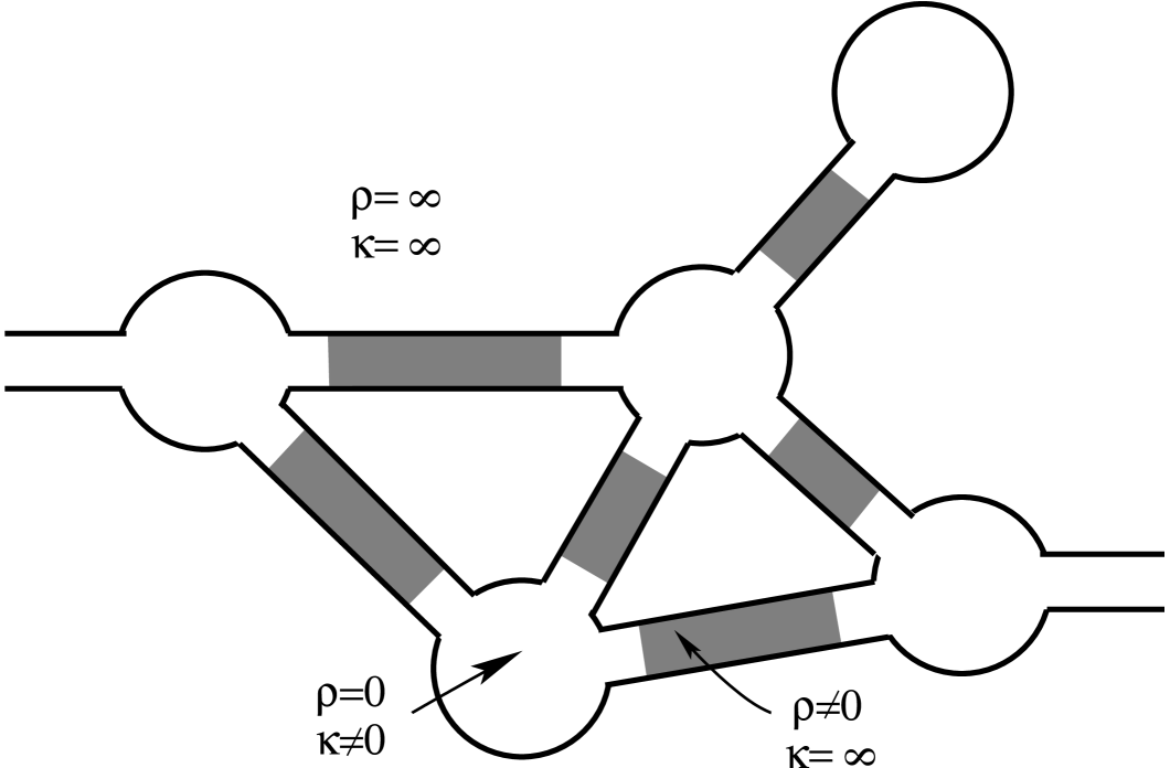
Figure 2: A two-terminal discrete acoustic network. In the idealized model the four cavities contain compressible massless fluid, while the grey shaded fluid plugs in the five tubes contain incompessible fluid with some mass.

Each entire cavity contains a compressible, non-viscous, massless fluid with compressibility possibly varying from cavity to cavity. In this model the compressibility is localized in the cavities and the mass is localized in the channels between cavities. The surfaces between the compressible and incompressible fluids are assumed to be flat and perpendicular to the channel. When one conceives an acoustic network, the area outside the network is assumed to be occupied by a rigid boby (or cladded by rigid tubes). However we can, in a equivalent way, assume that this area $\Omega_{0}$ is filled by an incompressible fluid having infinite density, i.e. with $\kappa=\rho=\infty$. Indeed, the infinite density, and the boundedness of $W(\Omega_{0})$ ensures that the velocity ${\bf v}$ (as one might physically expect) will be zero outside the network and consequently that the walls of the network remain fixed. The incompressibility ensures that both sides of (2.5) are zero in the matrix, without requiring that $P=0$ in the matrix. Hence the acoustic equation (2.5) desribes the system in the whole space.

In each entire cavity, $\Omega_{j}$, where $1/\rho$ is infinite (or more precisely is real positive and approaches infinity), $\nabla P$ must be zero, since otherwise $\rho|{\bf v}|^{2}=|\nabla P|^{2}/(\rho\omega^{2})$ would be infinite and $W(\Omega_{j})$ would be unbounded. Thus, as expected, the pressure is constant in each junction region. Within each segment of incompressible fluid of constant density, both sides of (2.5) must vanish, which implies $\nabla^{2}P=0$ in each such segment. From the boundary conditions (that $P$ is constant at the ends of the fluid segment, and at the sides ${\bf n}\cdot\nabla P=0$, since ${\bf n}\cdot{\bf v}=0$) it follows that the pressure $P$ will be constant in each cross section normal to the channel, and will vary linearly along the fluid segment. The fluid velocity ${\bf v}$ will therefore be constant in the segment, and directed parallel to the fluid channel. From (2.6) we see that in a channel joining cavity $i$ and cavity $j$ the fluid velocity in the direction of the channel, from $j$ to $k$ will be

$$v_{jk}=-[i/(\rho_{jk}\omega\ell_{jk})](P_{k}-P_{j}),$$ (2.8)

where $\ell_{jk}$ is the length of the fluid segment, $\rho_{jk}$ is its density and $P_{j}$ and $P_{k}$ are the complex pressures at junctions $j$ and $k$ respectively. This is basically Newton’s second law, relating the acceleration of the fluid segment, $-i\omega{\bf v}_{i,j}$, to its mass and the force acting on it.

In entire cavity $j$, (2.5) and (2.6) imply

$$\nabla\cdot{\bf v}=(i/\kappa)\omega P_{j},$$ (2.9)

which when integrated over the entire cavity implies, by the divergence theorem,

$$\sum_{k=1}^{m}hv_{jk}=a_{j}(i/\kappa_{j})\omega P_{j},$$ (2.10)

where $a_{j}$ is the area of the entire cavity, $\kappa_{i}$ is the bulk modulus of the fluid within it, and we have assumed that $m$ channels enter the cavity, each with width $h$ and carrying a fluid segment with velocity $v_{jk}$. This is essentially Hooke’s law, applied to the compressible fluid occupying the entire cavity. If the cavity is a terminal and there is an open channel carrying a current $I_{j}$ into it, then the relation (2.10) takes the modified form

$$I_{j}+\sum_{k=1}^{h}hv_{jk}=a_{j}(i/\kappa_{j})\omega P_{j}.$$ (2.11)

Given the pressures $P_{j}$ at the terminal cavities, the equations (2.8) and (2.10) provide a discrete set of equations, which can be solved for the pressures in the other cavities, the velocities of the fluid plugs in the channels, and the currents $I_{j}$ flowing into the terminal cavities. Assuming that the cavities are numbered in such a way that the first $n$ are terminals, and the remaining ones are not, the response of the network is expressed in terms of the linear relation

$${\bf I}={\bf M}{\bf P}$$ (2.12)

between the set of pressures ${\bf P}=\{P_{1},P_{2},\ldots,P_{n}\}$ at the terminals and the currents ${\bf I}=\{I_{1},I_{2},\ldots,I_{n}\}$ flowing into them.

Everything carries through to the electromagnetic case where the fields are transverse electric (TE). By comparing (2.5) and (2.6) with (2.1) and (2.2) we see that $\mu$ and $\varepsilon$ play the role of $\rho$ and $1/\kappa$; $E$ plays the role of $P$ and ${\bf H}$ plays the role of ${\bf R}_{\perp}{\bf v}$ (and is therefore perpendicular to the channel walls). The channels themselves are now thin plates containing a material with $\varepsilon=0$ and $\mu\neq 0$. The cavities are now aligned dielectric cylinders with $\varepsilon\neq 0$ and $\mu=0$. The electric field is constant in each cylinder, which also can be seen directly from the result of ?) who show that, for the dual transverse magnetic (TM) problem, cylinders having $\mu\neq 0$ and $\varepsilon=0$ have a constant magnetic field in them. It follows that ${\bf H}=0$ in the matrix by direct analogy with the acoustic case where ${\bf v}=0$ in the matrix. (Although magnetic fields tend to be concentrated inside a material with positive and very large permeability, this concentration refers to the ${\bf B}$ field and not to the ${\bf H}$ field).

We call such a circuit a transverse electric EM-circuit (see figure 3). Each equation we discussed has its analog. For example (2.11) becomes

$$I_{j}+\sum_{k=1}^{m}hH_{jk}=a_{j}i\omega\varepsilon_{j}E_{j},$$ (2.13)

where $H_{jk}$ is the value of ${\bf H}$ in the direction perpendicular to the walls of the plate $jk$, $I_{j}$ is the line integral of ${\bf H}$ across the open channel, $\varepsilon_{j}$ is the dielectric constant of cylinder $j$ while $E_{j}$ is the electric field in the cylinder $j$. So the left hand side of (2.13) is the line integral of ${\bf H}$ around the terminal dielectric cylinder, while the right hand side of (2.13) is the total displacement current flowing through the cylinder. Thus (2.13) is nothing but Ampere’s circuital law (with Maxwell’s correction). Notice that instead of having an open channel one could have a free current $-I_{j}$ flowing next to the terminal dielectric cylinder.

The analog of (2.8) is

$$H_{jk}=-[i/(\mu_{jk}\omega\ell_{jk})](E_{k}-E_{j}),$$ (2.14)

where $\mu_{jk}$ is the permeability of the plate $jk$. This is Faraday’s law of induction, relating the time derivative of flux of ${\bf B}$ through any rectangle with two opposite sides along the dielectric cylinders $j$ and $k$, to the line integral of ${\bf E}$ around this rectangle. Since ${\bf H}$ is constant and perpendicular to the plate walls, it follows from (2.2) that ${\bf E}$ in the plate depends linearly on $x_{1}$ and $x_{2}$ in such a way that it is constant perpendicular to the plate.

In the particular case when the cylinder $j$ has zero dielectric constant, i.e. $\varepsilon_{j}=0$, (so that the junction is the analog of a cavity filled with incompressible fluid) (2.13) becomes

$$I_{j}+\sum_{k=1}^{m}hH_{jk}=0,$$ (2.15)

where $I_{j}=0$ if the cylinder is not a terminal cylinder. If all cylinders have zero dielectric constant, then we call the circuit a transverse electric magnetic circuit (M-circuit).

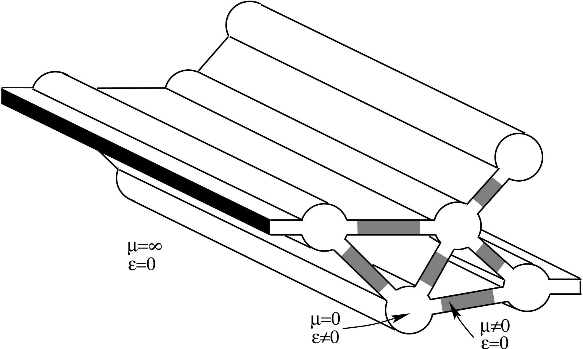
Figure 3: A two-terminal transverse electric EM-circuit which is the exact analog of the discrete acoustic network of Figure 1

It is now important to understand how can these circuits be used and in particular how they can interact with ordinary materials. The problem is analogous for connecting an acoustic discrete network to an ordinary acoustic three-dimensional domain. Assume that the matrix with $\mu=\infty$ and $\varepsilon=0$ only has finite extent, and is surrounded by space with $\mu=\varepsilon=1$, in which there are TE fields. Also suppose each terminal edge is connected to the exterior by an open channel, of width h, containing material with $\varepsilon=\mu=0$. The external field $E$ (which is the anolog of the pressure) will fix the mean value of $E_{j}$ at every open channel mouth $j$. Then the response of the transverse EM circuit will determine the values $I_{j}$, that is of ${\bf H}$ (which is analog to the velocity) at the open channel mouths. Let $\Omega_{0}$ denote the region occupied by the circuit plus the remaining matrix. On the part of the boundary of $\Omega_{0}$ which corresponds to the matrix we have ${\bf H}=0$. Hence the $E$-to-tangential value of ${\bf H}$ map (which is equivalent to the Dirichlet to Neumann map) of $\Omega_{0}$ will be governed by the response of the circuit. It will be completely different from a pure matrix (for which the tangential value of ${\bf H}$ vanishes on $\partial\Omega_{0}$) or from void where $\varepsilon=\mu=1$.

Note that the external field $E$ will fix the value of the electrical field at each open channel mouth in a efficient way if $h$ is large enough. If $h$ is too small this connection will be weak, and $E$ near each mouth will be strongly affected by flux of ${\bf R}_{\perp}{\bf H}$ (which is analogous to current in the acoustic setting) through the narrow channel openings. (In a region near but not too close to each mouth the $E$ field will be like that generated from a line source.) However this problem can be corrected by adding at each open channel mouth a material with $\varepsilon=\mu=0$ (see figure 4). Hence the value of $E$ at each mouth will be fixed by the value of $E$ on the ’relatively large’ cap boundary, and the flux of ${\bf R}_{\perp}{\bf H}$ through the channel will be transferred to the outside of the cap. This is similar to the way ?) has, for the dual TM problem, suggested the use of materials with $\varepsilon=0$ for transfering energy through narrow openings.

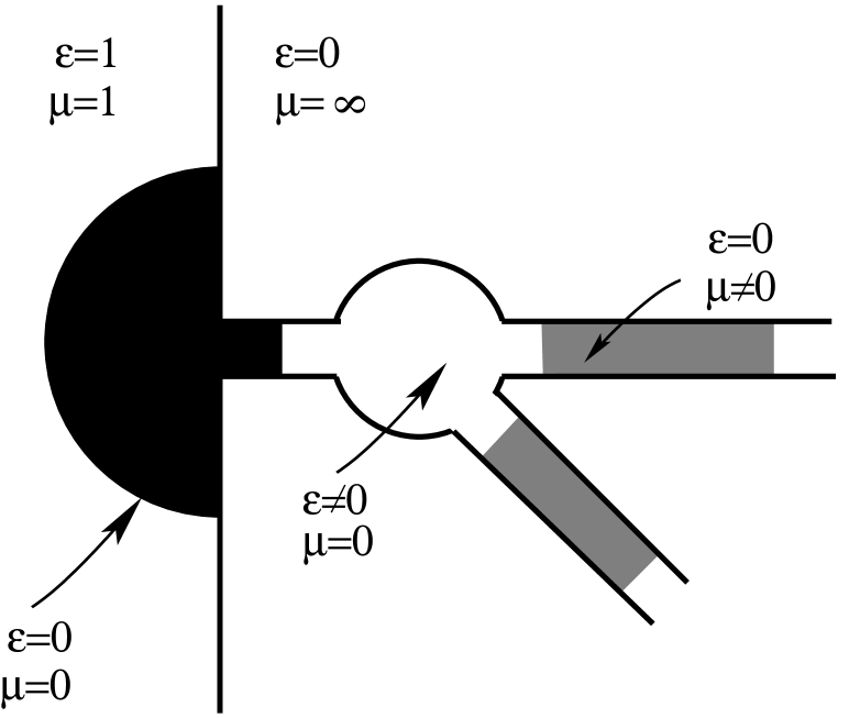
Figure 4: A semicircular plug of material with $\varepsilon=\mu=0$ can serve to couple the open channels of an transverse electric EM-circuit with exterior TE fields, allowing the ${\bf H}$ field to be transfered to the exterior with negligable drop in $E$.

3 Electromagnetic circuits in the general case

We need to generalize the EM-circuits to allow for fields that are not transverse electric. Like in the transverse electric case the circuit will be composed of plates of material having $\varepsilon=0$ and $\mu\neq 0$, joined by cylinders of dielectric material having $\varepsilon\neq 0$ and $\mu=0$, embedded in a matrix having $\mu=\infty$ and $\varepsilon=0$, so that the matrix is the electrodynamic equivalent of a void in elasticity according to (1.2)-(1.4).

The plates and the dielectric cylinders play the physical role in our circuits that springs and masses play in an elastic network, despite the fact that they are completely different geometrical objects. The assumption that the electromagnetic energy density in the matrix remains bounded as $\mu\to\infty$ and $\varepsilon\to 0$ when the moduli $\mu$ and $\varepsilon$ are positive and independent of frequency, again implies that ${\bf H}={\bf D}=0$ in the matrix. (Note that if ${\bf H}=0$ in the matrix then necessarily ${\bf D}=i\nabla\times{\bf H}/\omega$ is also zero).

We emphasize that when $\varepsilon$ and $\mu$ are real and positive in the matrix and $\mu$ is very large, while $\varepsilon$ is very small then there certainly exist (high energy) solutions where ${\bf H}$ in the matrix is not small: after all an electromagnetic wave could propagate there, and its amplitude scaled as one desires. However, we believe (and this needs to be rigorously verified) that the solutions in the matrix almost decouple from the solutions in the electromagnetic circuit when $\mu$ is very large and $\varepsilon$ is very small. This should be similar to the way electromagnetic fields almost decouple at a planar interface between two non-absorbing media, 1 and 2, for which there is a large mismatch in the electromagnetic impedances $\eta_{1}=\mu_{1}/\varepsilon_{1}$ and $\eta_{2}=\mu_{2}/\varepsilon_{2}$: when $\eta_{1}/\eta_{2}$ is very large then a plane electromagnetic wave incident from either side of the interface will have only a tiny portion of its energy transmitted.

Alternatively, and as kindly suggested to us by a referee, one may assume that in the matrix the product $\varepsilon\mu$ is large and negative. Then electromagnetic fields in the matrix will be confined within a small skin depth of the surface which tends to zero as $\varepsilon\mu\to-\infty$, again implying that ${\bf H}={\bf D}=0$ in the limit as $\mu\to\infty$ and $\varepsilon\to 0$ in such a way that $\varepsilon\mu\to-\infty$.

Let us now analyze in detail the response of each plate. The plate could be polygonal in shape, but for simplicity we use a basic element which is a very thin triangular prism, of uniform height $h$ containing a material having $\varepsilon=0$ and $\mu\neq 0$, the top and bottom faces of which are surrounded by the matrix, as illustrated in figure 5. We call this element a magnetic element.

Figure 5: A triangular prism containing material with $\varepsilon=0$ and $\mu\neq 0$ is one basic element of a magnetic or electromagnetic circuit. Here the arrows denote direction of the magnetic field ${\bf H}$ within the prism.

Let us choose our coordinate system so the bottom surface of the prism is at $x_{3}=0$ and the top surface at $x_{3}=h$. The triangle at the bottom of the prism has vertices $q$, $r$ and $s$, labeled in an anticlockwise order when viewed from above, and edges $qr$, $rs$ and $sq$. Let $\mu_{qrs}$ denote the constant value of $\mu$ within the prism. Since $\nabla\cdot{\bf H}=0$ and $\nabla\times{\bf H}=0$ in the prism it follows that ${\bf H}=\nabla\psi$ where $\Delta\psi=0$. Also since the tangential component of ${\bf H}=\nabla\psi$ is zero at the top and bottom surfaces of the prism, it follows that $\psi$ is constant on the top and bottom plates: $\psi$ is like the potential between two closely spaced capacitor plates. Hence ${\bf H}$ is essentially constant within the prism and normal to the top and bottom surfaces, i.e. ${\bf H}=(0,0,H_{3})$ where $H_{3}$ cannot depend on $x_{3}$ since $\nabla\cdot{\bf H}=0$ within the prism. (In fact ${\bf H}$ will only be approximately constant due to fringing fields which, however, should become negligible away from the edges, in the limit as the prism becomes very thin.)

Let ${\bf x}^{\prime}=(x_{1},x_{2})$ denote coordinates in the plane. Assuming the point $r$ is at $x_{1}=x_{2}=0$, the three edges of the triangle lie along the three lines

$${\bf x}^{\prime}=\alpha{\bf t}_{qr},\quad{\bf x}^{\prime}=\alpha{\bf t}_{rs},\quad{\bf x}^{\prime}={\bf x}^{\prime}_{0}+\alpha{\bf t}_{sq},$$ (3.1)

each parameterized by $\alpha$ where ${\bf t}_{mn}$ is the unit vector directed from vertex $m$ to vertex $n$, and ${\bf x}^{\prime}_{0}$ is a point along the edge $sq$. In electromagnetic circuits we constrain the tangential component of the electric field to take constant values $E_{qr}{\bf t}_{qr}$, $E_{rs}{\bf t}_{rs}$, and $E_{sq}{\bf t}_{sq}$ along the three sides $qr$, $rs$ and $sq$ of the triangle. (As we will see later the presence of dielectric cylinders along these edges will allow this constraint to be satisfied). Let $\ell_{qr}$, $\ell_{rs}$ and $\ell_{sq}$ denote the lengths of the edges $qr$, $rs$ and $sq$. Then Faraday’s law of induction applied to a circuit around the triangle implies

$$\ell_{qr}E_{qr}+\ell_{rs}E_{rs}+\ell_{sq}E_{sq}=ca_{qrs},$$ (3.2)

where $c=i\omega\mu_{qrs}H_{3}$ and $a_{qrs}$ is the area of the triangle.

To find an explicit expression for the electric field in the prism, although it is not clear we need it, let us assume that $\varepsilon$ in the prism is arbitrarily small, but non-zero (and many factors greater than the $\varepsilon$ in the matrix which we treat as being zero), so that in the prism $\nabla\cdot{\bf D}=0$ implies $\nabla\cdot{\bf E}=0$. Since ${\bf D}=0$ in the matrix and $\nabla\cdot{\bf D}=0$ it follows that ${\bf D}$ and hence ${\bf E}$ are tangential to the top and bottom surfaces of the prism.

Having a material with zero permittivity outside the prism allows us to have a non-zero ${\bf E}$ field there. Then the tangential components of ${\bf E}$ can be continuous across the top and bottom surfaces of the prism. It is not clear that this zero permittivity in the matrix is necessary. One could instead have $\varepsilon\neq 0$ and ${\bf E}=0$ outside the prism, with a concentrated surface ${\bf B}$ current to compensate for the jump in the tangential component of ${\bf E}$ across the surface. Such a concentrated surface ${\bf B}$ current should be allowed since $\mu=\infty$ in the matrix. (Similarly in an elastic network, it is not necessary that the surrounding material have density $\rho=0$, although that is the case when the surrounding material is void. If $\rho$ is non-zero and ${\bf C}$ is close to zero then only a small boundary layer near the elastic network will move.)

Since $\nabla\times{\bf E}=i\omega\mu{\bf H}$, we infer that

$${\bf E}=(-cx_{2}/2,cx_{1}/2,0)+\nabla\phi,$$ (3.3)

where $\Delta\phi=0$ and without loss of generality one can assume that $\phi=0$ at the origin. The potential $\phi$ satisfies the Neuman boundary conditions that ${\bf n}\cdot\nabla\phi=0$ on the top and bottom surfaces of the prism, and Dirichlet boundary conditions on the sides of the prism (specifying the tangential value of $\nabla\phi$ around the sides, and the value $\phi=0$ at the origin determines the value of $\phi$ along the sides). Thus $\phi$ is uniquely determined and a simple calculation using (3.1), the identity

$$\ell_{qr}{\bf t}_{qr}+\ell_{rs}{\bf t}_{rs}+\ell_{sq}{\bf t}_{sq}=0,$$ (3.4)

(as follows from the fact that the edges form a triangle) and the fact that $a_{qrs}=\ell_{sq}{\bf t}_{sq}\cdot{\bf R}_{\perp}{\bf x}_{0}/2$ is the area of the triangle (as can be easily seen by choosing ${\bf x}^{\prime}_{0}$ to be perpendicular to ${\bf t}_{sq}$ ) shows that the boundary conditions are satisfied with $\nabla\phi=(a_{1},a_{2},0)$ where ${\bf a}=(a_{1},a_{2})$ is constant and determined by

$${\bf t}_{qr}\cdot{\bf a}=E_{qr},\quad{\bf t}_{rs}\cdot{\bf a}=E_{rs}.$$ (3.5)

(The condition (3.2) ensures that ${\bf E}\cdot{\bf t}_{sq}=E_{sq}$ along the edge $sq$).

It is natural to introduce three new variables

$$V_{qr}=\ell_{qr}E_{qr},\quad V_{rs}=\ell_{rs}E_{rs},\quad V_{sq}=\ell_{sq}E_{sq},$$ (3.6)

which when $H_{3}=0$ would represent the potential drops along the three edges. Then (3.2) implies that $H_{3}$ depends on $V_{qr}$, $V_{rs}$, and $V_{sq}$ only through the sum $V_{qr}+V_{rs}+V_{sq}$.

In keeping with the vocabulary introduced in the introduction, the material surrounding the edges of the basic element exerts total applied surface free currents $J_{qr}^{s}$, $J_{rs}^{q}$ and $J_{sq}^{r}$ along the edges $qr$, $rs$ and $sq$, flowing in directions ${\bf t}_{qr}$, ${\bf t}_{rs}$, and ${\bf t}_{sq}$, where the superscript is kept to signify that the currents are associated with the triangle $qrs$. (Here total signifies that these are the applied surface free currents integrated over the width of each edge, but from now on this will be assumed so we will drop the word total). In other words, the boundary conditions on the edges of the basic element are essentially the same as if we completely surrounded the basic element by matrix material with $\varepsilon=0$ and $\mu\neq 0$ having ${\bf H}=0$ and inserted these surface free currents along the edges.

These currents are all equal, and from Ampere’s circuital law applied to a circuit around each edge take the value $hH_{3}$, by virtue of the fact that ${\bf H}$ is constant within the triangular prism. It may seem superfluous to keep track of the three currents $J_{qr}^{s}$, $J_{rs}^{q}$ and $J_{sq}^{r}$ when they are all equal. However, consider the analogous elastodynamic framework: to write the balance of forces at each node, one introduces the forces that each spring exerts on each node even though the forces exerted by a spring on its two extremity nodes are equal and opposite. Without introducing $J_{qr}^{s}$, $J_{rs}^{q}$ and $J_{sq}^{r}$ it would be difficult to derive an expression for the response matrix of an general electromagnetic circuit, as we do in section 5.

Thus we have the relation

$$\pmatrix{T_{qr}^{s}\cr T_{rs}^{q}\cr T_{sq}^{r}}\equiv\pmatrix{i\omega J_{qr}^{s}\cr i\omega J_{rs}^{q}\cr i\omega J_{sq}^{r}}=k_{qrs}\pmatrix{1&1&1\cr 1&1&1\cr 1&1&1\cr}\pmatrix{V_{qr}\cr V_{rs}\cr V_{sq}},$$ (3.7)

where $k_{qrs}=h/(a_{qrs}\mu_{qrs})$. We use the quantities $T$ rather than the free currents $J$ so that the matrix entering the above relation is real and so that the parallel with elastodynamics is maintained, since $i\omega{\bf j}$ in (1.2) plays the role of the body force ${\bf f}$ in (1.4).

Also our introduction of the variables $V$ rather than the variables $E$ ensures that the matrix is symmetric which is desirable since this property will then extend to the matrix describing the response of electromagnetic circuits with many elements. (Again, this is why it is important to introduce the three currents $J_{qr}^{s}$, $J_{rs}^{q}$ and $J_{sq}^{r}$ rather than just a single current.) This relation (3.7), which is essentially Faraday’s law of induction, is the analog of Hooke’s law,

$$\pmatrix{{\bf F}_{r}^{s}\cr{\bf F}_{s}^{r}}=k_{rs}\pmatrix{{\bf t}_{rs}\otimes{\bf t}_{rs}&-{\bf t}_{rs}\otimes{\bf t}_{rs}\cr-{\bf t}_{rs}\otimes{\bf t}_{rs}&{\bf t}_{rs}\otimes{\bf t}_{rs}\cr}\pmatrix{{\bf u}_{r}\cr{\bf u}_{s}},$$ (3.8)

describing the response of a spring, where ${\bf F}_{r}^{s}$ and ${\bf F}_{s}^{r}=-{\bf F}_{r}^{s}$ are the forces node $r$ and node $s$, respectively, exert on the spring joining these nodes, [which is the opposite of the definition given in ?)], ${\bf u}_{r}$ and ${\bf u}_{s}$ are the displacements at these two nodes, ${\bf t}_{rs}$ is the unit vector pointing from node $r$ to node $s$, and $k_{rs}$ is the spring constant. Note that the matrix entering both relations (3.7) and (3.8) is real, symmetric, degenerate and positive semidefinite. Also $i\omega J$ is playing the role of a force, and $1/\mu_{qrs}$ is playing the role of the elastic spring constant (to within a proportionality factor) as might be expected by comparing (1.2) and (1.4).

Figure 6: A magnetic circuit (M-circuit) is obtained by joining together a collection of triangular prisms, of the type illustrated in figure 5. At each edge there is a small diameter cylinder, not illustrated, having $\varepsilon=\mu=0$. Here the terminal edges are marked by thicker lines. An EM-circuit is obtained when a selection of the cylinders along the edges are assigned are a dielectric constant $\varepsilon\neq 0$.

A magnetic circuit (the analog of a elastic network with springs but no masses), as illustrated in figure 6, is a collection of such triangular prisms, joined at common edges by cylinders having $\mu=\varepsilon=0$ and with a constant diameter $d$ of the order of $h$. In fact it is desirable to take $\varepsilon$ in these cylinders arbitrarily small but non zero, since then ${\bf E}$ will be constant along the cylinder because ${\bf D}$ is (essentially) constant. Edges in such a magnetic circuit (M-circuit) play the role of nodes in an elastic network, and just as applied forces are confined to the terminal nodes in an elastic network, so too can applied free currents be confined to a subset of the edges in a magnetic circuit. We call these the terminal edges, and we call the others internal edges. If a magnetic circuit contains an internal edge $qr$ which is connected to only one triangle $qrs$, then $T_{qr}^{s}=T_{rs}^{q}=T_{sq}^{r}=0$ and the triangle $qrs$ can be removed without effecting the response of the network. (Analogously, if a spring network contains an internal node with only one spring and no mass attached to it then that spring can be removed without affecting the response of the network). Thus we can restrict attention to magnetic circuits where all internal edges are connected to at least two triangles.

Consider an internal edge $qr$ where $m$ triangles meet at a cylinder. Since $T_{qr}^{s}/(i\omega h)$ is the value of the constant magnetic field ${\bf H}$ within the triangular prism $qrs$, at an internal edge $qr$ where $m$ triangles meet at a cylinder, we have

$$\sum_{s=1}^{m}T_{qr}^{s}=0,$$ (3.9)

as follows from Ampere’s circuital law that the line integral of ${\bf H}$ around the cylinder is zero. Equation (3.9) is analogous to the balance of forces at a node in a spring network: the sum of all free currents must be zero if there is no net free current. At a terminal edge $qr$, Ampere’s circuital law implies

$$\sum_{s=1}^{m}T_{qr}^{s}=A_{qr},$$ (3.10)

where $A_{qr}/(i\omega)$ is the free current applied to that edge.

We label the edges in the network so that no edge is repeated twice, i.e. if $qr$ labels an edge in our list, then the label $rq$ does not appear in the list. This essentially assigns an arrow (from $q$ to $r$) to each edge, and it may be impossible to assign arrows so that no two arrows point to the same vertex in every triangle in the circuit. Accordingly, for example, we may want the relation (3.7) to involve $T^{q}_{sr}$ and $V_{sr}$ rather than $T^{q}_{rs}$ and $V_{rs}$ when the label $rs$ does not occur in the list. To eliminate the unwanted variables in (3.7) we can then use the relations

$$T^{q}_{rs}=-T^{q}_{sr},\quad V_{rs}=-V_{sr},$$ (3.11)

which hold for all $r$, $s$ and $q$. Thus (3.7) becomes

$$\pmatrix{T_{qr}^{s}\cr T_{sr}^{q}\cr T_{sq}^{r}}\equiv\pmatrix{i\omega J_{qr}^{s}\cr i\omega J_{rs}^{q}\cr i\omega J_{sq}^{r}}=k_{qrs}\pmatrix{1&-1&1\cr-1&1&-1\cr 1&-1&1\cr}\pmatrix{V_{qr}\cr V_{sr}\cr V_{sq}},$$ (3.12)

and still involves a real, symmetric, degenerate, positive semi-definite matrix.

To obtain an electromagnetic circuit from a magnetic circuit (including those magnetic circuits where some internal edges are only connected to one triangle) we assign a non-zero value to the dielectric constant (to some or all) of the cylinders, of diameter $d$, at the junctions of the triangles. (This is analogous to adding mass to the nodes of a spring network) An example is illustrated in figure 7. At any vertex where two or more dielectric cylinders meet we need to make sure there is a good electrical connection between the dielectric cylinders to allow displacement current to flow between the cylinders.

Figure 7: An electromagnetic circuit (EM-circuit) has small diameter dielectric cylinders with $\varepsilon\neq 0$ and $\mu=0$ along a selection of edges including possibly the terminal edges. Here there are three terminal edges are marked by thicker lines. The dielectric cylinders should be much thinner than drawn here. One internal edge, marked by the thin line, has a cylinder with $\varepsilon=\mu=0$ attached to it.

Now at an internal edge $qr$ where $m$ triangles meet at a dielectric cylinder the junction locally looks similar to the junction in a transverse electric EM circuit where $m$ plates meet at a dielectric cylinder, and so one expects an equation similar to (2.13) to hold. Ampere’s circuital law (with Maxwell’s correction) taken around a circuit surrounding the cylinder $qr$ implies

$$\sum_{s=1}^{m}T_{qr}^{s}=\omega^{2}g_{qr}V_{qr},$$ (3.13)

where $g_{qr}=\pi d^{2}\varepsilon_{qr}/(4\ell_{qr})$, in which $\varepsilon_{qr}$ is the dielectric constant of the cylinder. The term on the right arises from the fact that $-i(\pi d^{2}/4)\omega\varepsilon_{qr}E_{qr}$ is the total displacement current flowing through the dielectric cylinder. Inside the cylinder ${\bf D}=\nabla\chi$ (since $\nabla\cdot{\bf D}=0$ and $\nabla\times{\bf E}=0$) where ${\bf n}\cdot\nabla\chi=0$ at the cylinder walls (since ${\bf D}=0$ in the matrix and in the triangular elements). At the cylinder ends one has some flux of ${\bf D}$. From the solution to this Neumann problem ${\bf D}$ will be essentially constant inside the small diameter cylinder away from the ends. This justifies our assumption that the electric field takes constant values along the edges of a magnetic triangular element, at least when there are dielectric cylinders along each of these edges.

The equation (3.13) which is essentially the same as (2.13) when $I_{j}=0$, is the analog in an elastic network of Newton’s law,

$$\sum_{s=1}^{m}{\bf F}_{r}^{s}=\omega^{2}m_{r}{\bf u}_{r},$$ (3.14)

describing the motion of a mass $m_{r}$ at a node $r$ where $m$ springs meet. At a terminal edge (3.13) generalizes to

$$\sum_{s=1}^{m}T_{qr}^{s}=A_{qr}+\omega^{2}g_{qr}V_{qr}$$ (3.15)

where again $A_{qr}/(i\omega)$ is the free current applied to that edge. The equations (3.7), (3.13), and (3.15) hold for each triangle and each edge, and provide a system of equations which can be solved to determine the response of an arbitrary electromagnetic circuit. This will be done in section 5.

The mathematical idealization of an electromagnetic circuit is obtained by taking the limits $h\to 0$ and $d\to 0$, while say keeping the ratio $d/h$ fixed. The moduli of the constituent materials need to be scaled in such a way that the parameters entering the final equations, such as $k_{qrs}$ and $g_{qr}$, remain fixed. Thus one should take $\mu_{qrs}$ proportional to $h$ (and thus very small) and $\varepsilon_{qr}$ proportional to $1/d^{2}$ (and thus very large).

4 Acting upon an electromagnetic circuit and creating virtual free currents

One might ask how one could conceivably act on an EM-circuit, and measure its response. A possible scenario, as sketched in figure 8, might be to be to have electromagnetic fields incident on a body, say a cube, of material with $\mu=\infty$ and $\varepsilon=0$ containing an EM-circuit, with no two terminal edges sharing a common vertex, positioned in such a way that only the terminal edges are exposed at the surface of the cube. Let us suppose that there are no dielectric cylinders attached to the terminal edges. Then the electric field will not be constant along each terminal edge. If $qr$ is a terminal edge between points $q$ and $r$ both on the same face of the cube, then Faraday’s law of induction implies that the line integral of ${\bf E}$ along that terminal edge will play the role of the quantity $V_{qr}$ in the electromagnetic circuit so that (3.7) remains satisfied.

Figure 8: A cube of material with $\mu=\infty$ and $\varepsilon=0$ containing an EM-circuit with four terminal edges exposed on the faces of the cube. From the outside it will look as if there are free currents flowing along the terminal edges (although in reality they do not exist) with the endpoints acting as sources and sinks for the displacement current field outside the cube. These virtual free currents will be generated according to the values of the line integrals of ${\bf E}$ along the terminal edges, and according to the response matrix of the EM-circuit. In the dual setting, it will look like a ME-circuit generates virtual magnetic monopole currents.

The EM-circuit causes the magnetic field ${\bf H}$ outside the body to be altered in such a way that Ampere’s circuital law (with Maxwell’s corrections) holds around each terminal edge. If one was not aware of the existence of the EM-circuit, from outside the body it would look as if the magnetic field ${\bf H}$ near the terminal edge $qr$ was generated by a free-current $-A_{qr}/(i\omega)$ flowing from $q$ to $r$. In other words, if one incorrectly assumes that ${\bf H}=0$ throughout the cube, then Ampere’s circuital law would falsely imply the existence of this free current, which we call a virtual free current, flowing along the terminal edge. It is nothing else but the surface free current which the EM-circuit exerts on the surrounding material at the terminal edge $qr$. (In a similar fashion one can insert a mass-spring network into a cavity in an elastic body, with only the terminal nodes attached to the boundary of the cavity. If one is not aware of the existence of the spring mass network from outside the cavity, it would look like the stress field in the body was altered by concentrated forces acting at the positions of the terminal nodes.)

Now the internal edges will carry some displacement current $A_{qr}/(i\omega)$ out of the vicinity of the point $q$ and a displacement current $A_{qr}/(i\omega)$ into the vicinity of $r$. If one is not aware of the existence of the electromagnetic circuit it would look like the point $p$ is a current source and the point $r$ is a current sink: it would look like the ends of the virtual free-current $-A_{qr}/(i\omega)$ along the terminal edge, act as sources and sinks for the displacement current outside the body.

If the thickness $h$ of each terminal edge is very small, then the coupling between the electromagnetic circuit and the fields in the exterior will be weak. As in the case of transverse electric EM-circuits, small virtual free-currents along the terminal edges will cause the field ${\bf E}({\bf x})$ to be modified in the near vicinity of each terminal edge. One suggestion to enhance the coupling is cap each terminal edge $qr$ with a $\varepsilon=\mu=0$ semicircular cylinder of length $\ell_{qr}$ and diameter $d_{0}$, where $d_{0}$ is not small. At the two ends of this cylinder one could attach $\varepsilon=\infty$, $\mu=0$ quarter spheres of diameter $d_{0}$, to allow the displacement current to enter and exit the points $q$ and $r$ with little resistance. In these quarter spheres ${\bf E}=0$. Faraday’s law of induction then implies that the line integral of ${\bf E}$ along the outer surface of the semicircular cylinder will equal the line integral of ${\bf E}$ along the terminal edge.

5 A formula for the response matrix of an EM-circuit, and the properties of this response matrix

In a magnetic or electromagnetic circuit with $n$ terminal edges let us suppose these edges have been numbered from $1$ to $n$. Then the response of the network is governed by the linear relation

$${\bf A}={\bf W}{\bf V}$$ (5.1)

between the terminal variables ${\bf A}=(A_{1},A_{2},\ldots,A_{n})$ which measure the real or virtual free currents at these edges, and the variables ${\bf V}=(V_{1},V_{2},\ldots,V_{n})$ which measure the line integral of the electric field along these edges. When all the edges in the circuit are terminal edges the response matrix ${\bf W}$ equals a symmetric matrix ${\bf W}^{0}$ with an especially simple form. From (3.7) and (3.15) the diagonal elements of ${\bf W}^{0}$ are given by

$$W^{0}_{qr,qr}=-\omega^{2}g_{qr}+\sum_{s}k_{qrs},$$ (5.2)

where the sum is over vertices $s$ such that $qrs$ is a triangle in the circuit, while the off-diagonal elements $W^{0}_{qr,st}$ are zero when $qr$ and $st$ are not two edges of some triangle in the circuit, and the remaining off diagonal elements are each given by one of the formulas

$$W^{0}_{qr,rs}=W^{0}_{qr,sq}=k_{qrs},\quad W^{0}_{qr,sr}=W^{0}_{qr,qs}=-k_{qrs},$$ (5.3)

according to what edge labels are in our list, where $qrs$ is a triangle in our circuit. Suppose we divide these edges into two groups, and order the edges so that one group comes first. Then the matrix relation (5.1) takes the block form

$$\pmatrix{{\bf A}_{1}\cr{\bf A}_{2}}=\pmatrix{{\bf W}^{0}_{11}&{\bf W}^{0}_{12}\cr({\bf W}^{0}_{12})^{T}&{\bf W}^{0}_{22}}\pmatrix{{\bf V}_{1}\cr{\bf V}_{2}},$$ (5.4)

where ${\bf A}_{1}$ and ${\bf V}_{1}$ are the set of variables associated with the first group and ${\bf A}_{2}$ and ${\bf V}_{2}$ are the set of variables associated with the second group. Now consider the case where the first group are terminal edges, while the second group are internal edges. Then ${\bf A}_{2}=0$ and (5.4) implies ${\bf A}_{1}={\bf W}{\bf V}_{1}$ with the response matrix ${\bf W}$ of the circuit being the Schur complement

$${\bf W}={\bf W}^{0}_{11}-{\bf W}^{0}_{12}({\bf W}^{0}_{22})^{-1}({\bf W}^{0}_{12})^{T}.$$ (5.5)

This is our formula for the response matrix of an arbitrary electromagnetic circuit. In particular it shows that the response matrix is always symmetric. It may be that the matrix ${\bf W}^{0}_{22}$ is singular, in which case if ${\bf A}_{1}$ is finite there are generally restrictions on the possible values that ${\bf V}_{1}$ can take.

Also recall that the matrix entering the relation (3.7) is positive semidefinite. Therefore if $\mu_{qrs}$ has a non-negative imaginary part, and hence $k_{qrs}$ has a non-positive imaginary part, for each triangle $qrs$ in the circuit and $\varepsilon_{qr}$, and hence $g_{qr}$, have a non-negative imaginary part for each edge $qr$ in the circuit, the imaginary part of ${\bf W}^{0}$ will be negative semidefinite, being a sum of negative semidefinite matrices. It follows that the quantity

$$S={\bf A}^{\prime}\cdot{\bf V}^{\prime\prime}-{\bf A}^{\prime\prime}\cdot{\bf V}^{\prime}=-{\bf V}^{\prime}\cdot({\bf W}^{0})^{\prime\prime}{\bf V}^{\prime}-{\bf V}^{\prime\prime}\cdot({\bf W}^{0})^{\prime\prime}{\bf V}^{\prime\prime}$$ (5.6)

will be non-negative, where the primes denote real parts, and the double primes imaginary parts. In particular if ${\bf A}_{2}$ in (5.4) is zero, the left hand side of the above equation reduces to

$$S={\bf A}_{1}^{\prime}\cdot{\bf V}_{1}^{\prime\prime}-{\bf A}_{1}^{\prime\prime}\cdot{\bf V}_{1}^{\prime}=-{\bf V}_{1}^{\prime}\cdot{\bf W}^{\prime\prime}{\bf V}_{1}^{\prime}-{\bf V}_{1}^{\prime\prime}\cdot{\bf W}^{\prime\prime}{\bf V}_{1}^{\prime\prime},$$ (5.7)

and since this is non-negative for all values of ${\bf V}_{1}$ we deduce that ${\bf W}^{\prime\prime}$, like $({\bf W}^{0})^{\prime\prime}$, is negative semidefinite.

6 The energy stored and dissipated in an electromagnetic circuit

To obtain a formula for the time averaged energy stored in an electromagnetic circuit let us assume the moduli in the electromagnetic circuit are real and do not depend on frequency. Recall that the physical electric and magnetic fields are the real part of ${\bf E}e^{-i\omega t}$ and ${\bf H}e^{-i\omega t}$. Locally the time averaged electric and magnetic field energy densities will therefore be $\varepsilon|{\bf E}|^{2}/4$ and $\mu|{\bf H}|^{2}/4$. In the magnetic element $qrs$ discussed at the beginning of section 3 the time averaged stored magnetic energy will be

$$ha_{qrs}\mu_{qrs}|H_{3}|^{2}/4=|T_{qr}^{s}|^{2}/(4\omega^{2}k_{qrs}),$$ (6.1)

while in the dielectric cylinder $qr$ the time averaged stored electrical energy will be

$$(\pi\ell_{qr}d^{2}/4)\varepsilon_{qr}|E_{qr}|^{2}/4=|V_{qr}|^{2}g_{qr}/4.$$ (6.2)

The total electromagnetic energy stored in the electromagnetic circuit will be a sum of such expressions taken over all magnetic elements and dielectric cylinders in the circuit. An appealing feature is that the resultant expression only depends on $\omega$ and the parameters $T$, $V$, $k$ and $g$ characterizing the electromagnetic circuit, and not on the parameters $a_{qrs}$, $h$, $\ell_{qr}$, and $d$.

Now let us consider how much electromagnetic energy is dissipated into heat within the electromagnetic circuit when the moduli are complex and depend on frequency. Locally the time averaged electrical and magnetic power dissipated into heat per unit volume will be $\omega\varepsilon^{\prime\prime}|{\bf E}|^{2}/2$ and $\omega\mu^{\prime\prime}|{\bf H}|^{2}/2$, respectively. Within the magnetic element $qrs$ this will integrate to

$$\omega ha_{qrs}\mu_{qrs}^{\prime\prime}|H_{3}|^{2}/2 = (1/k_{qrs})^{\prime\prime}|T_{qr}^{s}|^{2}/(2\omega)$$ (6.3)

$$= [(T_{qr}^{s})^{\prime}(T_{qr}^{s}/k_{qrs})^{\prime\prime}-(T_{qr}^{s})^{\prime\prime}(T_{qr}^{s}/k_{qrs})^{\prime}]/(2\omega).$$

Now we can substitute (3.7) into this, and associate a portion of the resultant expression to each edge, where the portion assigned to edge $qr$ is

$$[(T_{qr}^{s})^{\prime}V_{qr}^{\prime\prime}-(T_{qr}^{s})^{\prime\prime}V_{qr}^{\prime}]/(2\omega).$$ (6.4)

In the dielectric cylinder $qr$ the time averaged electrical power dissipated into heat is

$$(\pi\ell_{qr}d^{2}/4)\omega\varepsilon_{qr}^{\prime\prime}|E_{qr}|^{2}/2 = \omega|V_{qr}|^{2}g_{qr}^{\prime\prime}/2$$ (6.5)

$$= [(-\omega^{2}g_{qr}V_{qr})^{\prime}V_{qr}^{\prime\prime}-(-\omega^{2}g_{qr}V_{qr})^{\prime\prime}V_{qr}^{\prime}]/(2\omega).$$

Adding up all the contributions (6.4) and (6.5) associated with edge $qr$ and using the relation (3.15) we see that the total contribution associated with edge $qr$ is zero for an internal edge and

$$[A_{qr}^{\prime}V_{qr}^{\prime\prime}-A_{qr}^{\prime\prime}V_{qr}^{\prime}]/(2\omega)$$ (6.6)

for a terminal edge. By summing this expression over all terminal edges we see that the quantity $S/(2\omega)$, where $S$ is given by (5.7), is the time averaged electromagnetic energy converted into heat in the circuit.

This is consistent with Poynting’s theorem. Suppose we attached to the edge $qr$ a rectangular plate of thickness $h$ and width $\ell_{qr}$ in which there is a magnetic field ${\bf H}$ with component $H_{qr}=-A_{qr}/(i\omega h)$ perpendicular to the plate (and

surrounded by material with $\mu=\infty$ and $\varepsilon=0$) so that Ampere’s circuital law (with Maxwell’s corrections) is satisfied around the terminal edge. At any instant in time the flux of energy into the terminal $qr$ will be $h\ell_{qr}(E_{qr}e^{-i\omega t})^{\prime}(H_{qr}e^{-i\omega t})^{\prime}$, so the time averaged energy flux is

$$h\ell_{qr}(E_{qr}^{\prime}H_{qr}^{\prime}+E_{qr}^{\prime\prime}H_{qr}^{\prime\prime})/2=(-V_{qr}^{\prime}A_{qr}^{\prime\prime}+V_{qr}^{\prime\prime}A_{qr}^{\prime})/(2\omega).$$ (6.7)

Thus the quantity (6.6) has the physical interpretation as this time averaged energy flux, and it is then natural that its sum over all terminal edges should be the time averaged electromagnetic energy converted into heat in the circuit.

7 A correspondence between electrical circuits and a subclass of electromagnetic circuits

At fixed frequency, linear electrical circuits correspond to a subclass of EM-circuits, namely those where there are a sufficient number of magnetic elements and these all have $\mu_{qrs}=0$. Let us consider, for simplicity, an $n$-terminal planar electrical network with terminal nodes at the vertices of a polygon and with the remainder of the circuit lying with the polygon. If $J_{qr}$ is the complex current flowing from node $q$ to node $r$ and these nodes have complex voltages $V_{q}$ and $V_{r}$, then we have

$$J_{qr}=Y_{qr}(V_{q}-V_{r}),$$ (7.1)

where $Y_{qr}$ is the complex admittance (having non-negative real part) of the circuit element joining these two nodes.

Figure 9: Construction of an EM-circuit corresponding to the planar electrical 4-terminal network (a). The first step in (b) is to triangulate the network, and place appropriately valued dielectric cylinders (not shown) along the edges, and magnetic triangles with $k=\infty$ in each triangle. Then one adds a vertex below the network, and magnetic triangles with $k=\infty$ on the four triangular sides. The four new edges, marked by thicker lines, are the terminal edges of the EM-circuit.

For example, one may consider the four terminal network of figure 9(a) which has two internal nodes. To build an associated EM-circuit, the first step is to triangulate the network by adding additional edges with zero admittance, as illustrated in 9(b). To each triangle formed by this triangulation (not containing any nodes) with vertices $q$, $r$ and $s$ we assign a constant $k_{qrs}=\infty$. In the limit as $k_{qrs}\to\infty$ the equation (3.7) reduces to

$$T_{qr}^{s}=T_{rs}^{q}=T_{sq}^{r},\quad V_{qr}+V_{rs}+V_{sq}=0.$$ (7.2)

Following the ideas of ?) and ?) we attach to each edge $qr$ a dielectric cylinder with constant $g_{qr}=iY_{qr}/\omega$, which therefore will have non-negative imaginary part. [If the circuit element is a capacitor, then this will correspond to taking a value of the dielectric constant $g_{qr}$ which is real and positive; if the circuit element is a resistor, then this will correspond to taking $g_{qr}$ with zero real part and positive imaginary part; if the circuit element is an inductor, then this will correspond to taking $g_{qr}$ almost real and negative.]

The equation (3.13) then becomes

$$J_{qr}=Y_{qr}V_{qr},\quad{\rm where}~{}J_{qr}=\frac{1}{i\omega}\sum_{s=1}^{m}T^{s}_{qr}=\sum_{s=1}^{m}J^{s}_{qr},$$ (7.3)

in which $m=1$ or $2$ is the number of triangles sharing the edge $qr$, and $s$ indexes each of these triangles.

We next introduce an additional node 0 below the network, and for each pair $t$ and $u$ of neighboring terminal nodes around the polygon we construct the triangle $tu0$ with constant $k_{tu0}=\infty$. As illustrated in figure 9(c). This implies we have

$$T_{tu}^{0}=T_{u0}^{t}=T_{0t}^{u},\quad V_{tu}+V_{u0}+V_{0t}=0.$$ (7.4)

The edges $u0$, with $u=1,2,\ldots n$ are taken as the terminal edges of the electrodynamic circuit, and no dielectric cylinders are attached to them. The second equations in (7.2) and (7.4) imply that we can assign a voltage $V_{q}$ to each node such that

$$V_{qr}=V_{q}-V_{r},\quad V_{0}=0,\quad V_{u0}=V_{u}.$$ (7.5)

Thus (7.3) reduces to (7.1). Also the first equations in (7.2) and (7.4) ensure that the total current is a sum of loop currents. Therefore Kirchoff’s law that the sum of currents flowing into a node equals the sum of currents flowing out of that node is automatically satisfied. Thus the standard electrical circuit equations are satisfied.

Now the terminal edge variables $V_{u0}$, $u=1,2,\ldots n$, are the voltages at the terminal nodes of the electrical circuit. Also it is easy to see that the terminal edge variable $J_{u0}=A_{u0}/(i\omega)$ is the net current flowing out of the electrical circuit from node $u$ to node $0$. Thus the map ${\bf W}/(i\omega)$ is the Dirichlet to Neumann map of the electrical circuit.

If the electrical circuit is non-planar, then we modify the circuit so that all the terminal nodes are at the vertices of a (not necessarily convex) polygon lying on a plane below the circuit. Then the circuit above the plane is appropriately triangulated by adding additional nodes if necessary. A magnetic element with $k=\infty$ is inserted in each triangle and appropriately valued dielectric cylinders are attached to the edges. Each pair of neighboring terminal nodes on the polygon are then attached with a magnetic element having $k=\infty$ to an additional ground node situated below the plane. Each edge between a terminal node and the ground node is a terminal edge of the resulting EM-circuit.

8 Electromagnetic ladder networks, a characterization of their possible response matrices, and a material with non-Maxwellian macroscopic behavior

Electromagnetic circuits can have many different topologies and seems very difficult to characterize their possible macroscopic matrices ${\bf W}$, i.e. classify (for a given topology of terminal edge connections?) which matrices are realizable as the Schur complement of a matrix ${\bf W}^{0}$ with elements (5.2) and (5.3), and which ones not. Here we restrict our attention to an important subclass of electromagnetic circuits, called electromagnetic ladder networks (EM ladder networks), for which such a characterization is possible. Consider, as illustrated in the simple EM-circuit consisting of two magnetic triangles $qrs$ and $rst$ joined by a cylinder with $\varepsilon=\mu=0$ along the internal edge $rs$. Assume they have the same constant $k_{qrs}=k_{rst}=k$. Then (3.7) implies

$$T_{qr}^{s} = T_{rs}^{q}=T_{sq}^{r}=k(V_{qr}+V_{rs}+V_{sq}),$$

$$T_{rs}^{t} = T_{st}^{r}=T_{tr}^{s}=k(V_{rs}+V_{st}+V_{tr}).$$ (8.1)

The edges $sq$ and $tr$, labeled 1 and 2, are taken to be the terminal edges. They are without dielectric cylinders, so (3.15) and (3.13) imply

$$T_{sq}^{r}=A_{sq}\equiv-I_{12},\quad T_{tr}^{s}=A_{tr}\equiv-I_{21},\quad T_{rs}^{q}+T_{rs}^{t}=0.$$ (8.2)

Suppose there are dielectric cylinders along the internal edges $qr$ and $st$ with the same constants $g_{qr}=g_{st}=g$. At these edges (3.13) implies

$$T_{qr}^{s}=\omega^{2}gV_{qr},\quad T_{st}^{r}=\omega^{2}gV_{st}.$$ (8.3)

Solving these equations for $I_{12}$ and $I_{21}$ in terms of $V_{1}\equiv V_{sq}$ and $V_{2}\equiv V_{tr}$ gives

$$I_{12}=-I_{21}=k_{12}(V_{2}-V_{1}),$$ (8.4)

where

$$k_{12}=\frac{1}{2}[1/k-1/(\omega^{2}g)]^{-1}$$ (8.5)

has non-positive imaginary part, because $k$ has non-positive imaginary part and $g$ has non-negative imaginary part. From now on we ignore the internal edges of this simple EM-circuit, treating the simple EM-circuit itself as a basic ladder network element.

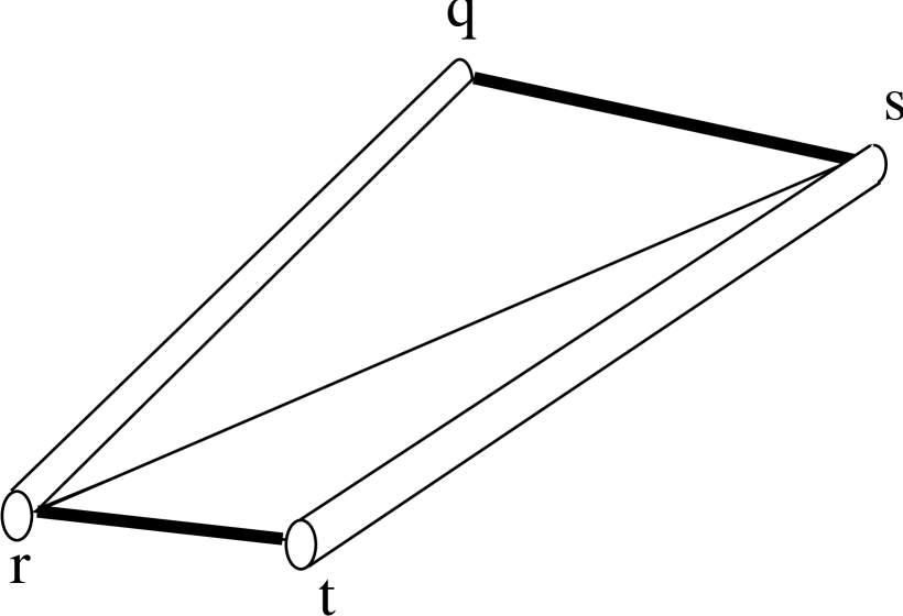
Figure 10: A simple EM-circuit which is the basic element for constructing EM ladder networks. The triangles $qrs$ and $rst$ are magnetic elements, and dielectric cylinders are attached to the edges $qr$ and $st$. A cylinder, not shown, with $\varepsilon=\mu=0$ is attached to the edge $rs$ to join the two magnetic elements. The edges $rt$ and $qs$ (which need not be coplanar) are terminal edges.

The relation (8.4) is similar to that associated with an element in an electrical circuit, although the physical interpretation of the variables is completely different. In the setting of an electrical circuit, using the notation of ?), 1 and 2 label two nodes, $V_{1}$ and $V_{2}$ are the potentials at these nodes, $iI_{12}/\omega$ is the current flowing from node 1 to node 2, while $iI_{21}/\omega$ is the current flowing from node 2 to node 1, and $k_{12}=1/L$ for an inductor, $k_{12}=-\omega^{2}C$ for a capacitor, and $k_{12}=-i\omega/R$ for a resistor, where $L$ is the inductance, $C$ the capacitance, and $R$ the resistance.

Building upon this analogy we can join a set of these simple EM circuits together, to obtain what we call an EM ladder network, as illustrated in figure 11(a). An $n$-terminal EM ladder network consists of $n+m$ edges $Q_{\alpha}$ indexed by $\alpha=1,2,\ldots,n+m$, having no vertex in common. Each pair of edges $(Q_{\alpha},Q_{\beta})$ may have a simple EM-circuit (of the type just discussed) joining them, and from (8.4), we have the relation

$$I_{\alpha\beta}=-I_{\beta\alpha}=k_{\alpha\beta}(V_{\beta}-V_{\alpha}),$$ (8.6)

where $k_{\alpha\beta}$ is the constant associated with the simple EM-circuit, and $k_{\alpha\beta}=0$ if there is no simple EM-circuit joining the edges. The first $n$ edges $Q_{\alpha}$ are the terminal edges of the EM ladder network (not to be confused with the terminal edges of the simple EM-circuits, which are all the edges $Q_{\alpha}$), and the remaining $m$ edges are internal edges.

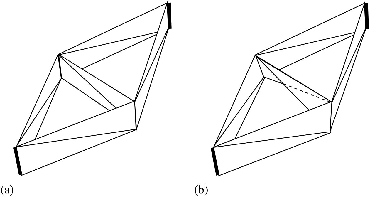
Figure 11: Figure (a) shows an EM ladder network which is the analog of the classical Wheatstone bridge, although its physical behavior is completely different. The two terminal edges are marked by the thicker lines, and for simplicity the dielectric cylinders along the edges of each basic ladder network element are not shown. Dielectric cylinders could be inserted along the edges between neighboring basic ladder network elements, in which case the EM ladder network becomes equivalent of a Wheatstone bridge with each node connected by a capacitor to ground. In figure (b) we have twisted the central bridge element so that it has a response governed by (8.9)

Each pair of edges $(Q_{\alpha},Q_{\beta})$ may have an elementary EM-circuit of the type just discussed joining them. Each edge $Q_{\alpha}$, may have a dielectric cylinder, with constant $g_{\alpha}$ attached to it. If this edge is an internal edge of the EM ladder network then from (3.13) we have

$$\sum_{\beta=1}^{n+m}I_{\alpha\beta}=-\omega^{2}g_{\alpha}V_{\alpha},$$ (8.7)

(in which we set $I_{\alpha\alpha}=0$) while if this edge is a terminal edge of the EM ladder network then from (3.15) we have,

$$A_{\alpha}+\sum_{\beta=1}^{n+m}I_{\alpha\beta}=-\omega^{2}g_{\alpha}V_{\alpha}.$$ (8.8)

The response of the EM ladder network is then governed by the relation ${\bf A}={\bf W}{\bf V}$ between the terminal variables ${\bf A}=(A_{1},A_{2},\ldots,A_{n})$ which measure the free currents at these edges, and the variables ${\bf V}=(V_{1},V_{2},\ldots,V_{n})$ which measure the tangential electric field at these edges.

Equations (8.6)-(8.8) are the same as those for electrical circuit in which the nodes may be connected to ground by a capacitor. It then follows directly from the results of ?) that for any fixed real frequency $\omega$ any real symmetric matrix ${\bf W}$ may be realized by an EM ladder network having real positive values of the constants $k_{\alpha\beta}$ and $g_{\alpha}$, and any complex symmetric matrix ${\bf W}$ with ${\rm Im}{\bf W}\geq 0$ can be realized by an EM ladder network having real positive values of the constants $k_{\alpha\beta}$ and complex values of the constants $g_{\alpha}$ having non-negative real and imaginary parts. Thus at fixed frequency we have a complete characterization of the possible response matrices ${\bf W}$ of EM ladder networks, both in the lossless case, and in the lossy case. We also have a complete characterization of the possible response matrices ${\bf W}$ associated with the class of electromagnetic circuits where no two terminal edges are connected, since an EM ladder network can be constructed having these edges as its terminals, and having the desired response matrix ${\bf W}$.

We can introduce another basic ladder network element of an EM ladder network. Just by reversing the roles of the vertices $t$ and $r$ in the original basic ladder network element and using (3.11), we obtain a basic ladder network element with the response

$$I_{12}=I_{21}=-k_{12}(V_{1}+V_{2}).$$ (8.9)

Of course utilizing such basic ladder network elements, as done in the example of figure 11(b), does not enlarge the class of possible response matrices ${\bf W}$ of EM ladder networks at fixed frequency (which is already as large as possible without the introduction of such elements).

Let us now sketch how one could get a material with non-Maxwellian macroscopic behavior using electromagnetic ladder networks. In the same way that one can build a cubic network of resistors so too can one build a cubic EM ladder network of basic network elements with the response (8.6) joined at edges $Q_{\alpha}$, with no dielectric cylinders attached to these edges (so that all $g_{\alpha}=0$ and it corresponds to the cubic network of resistors). Just as the cubic network of resistors responds macroscopically as a material with some effective conductivity, so too will the cubic EM ladder network respond macroscopically in a way which is definitely non-Maxwellian. Without being too specific, for a periodic ladder network one will have some relation of the form ${\bf K}=\mbox{\boldmath${\Sigma}$}\nabla V$, where $V({\bf x})$ is a suitably scaled local average of the variables $V_{\alpha}$, ${\Sigma}$ is the matrix governing the effective response, and $K_{i}({\bf x})$, $i=1,2,3$, is a suitably scaled local average of the variables $I_{\alpha\beta}$ taken over the subset of basic ladder network elements which are “aligned” parallel to the $x_{i}$-axis. If such a cubic EM ladder network is embedded in a large cube having $\mu=\infty$ and $\varepsilon=0$ with the terminal edges exposed at the boundary of the cube, then the interface conditions between the electromagnetic fields outside the cube, and the fields ${\bf K}({\bf x})$ and $V({\bf x})$ inside the cube will presumably depend on the geometric microconfiguration of the terminal edges of the EM ladder network at the cube faces. Obviously there is much to explore here.

References

- 1
- Alibert, dell’Isola, and Seppecher (2003 Alibert, J.-J., F. dell’Isola, and P. Seppecher 2003. Truss modular beams with deformation energy depending on higher displacement gradients. Mathematics and Mechanics of Solids 8(1):51–74.
- Bouchitté and Bellieud (2002 Bouchitté, G. and M. Bellieud 2002. Homogenization of a soft elastic material reinforced by fibers. Asymptotic Analysis 32(2):153–183.
- Briane (1998 Briane, M. 1998. Homogenization in some weakly connected domains. Ricerche di Matematica (Napoli) 47(1):51–94.
- Briane (2002 Briane, M. 2002. Homogenization of non-uniformly bounded operators: critical barrier for nonlocal effects. Archive for Rational Mechanics and Analysis 164(1):73–101.
- Briane and Mazliak (1998 Briane, M. and L. Mazliak 1998. Homogenization of two randomly weakly connected materials. Portugaliae Mathematica 55(2):187–207.
- Camar-Eddine and Seppecher (2002 Camar-Eddine, M. and P. Seppecher 2002. Closure of the set of diffusion functionals with respect to the Mosco-convergence. Mathematical Models and Methods in Applied Sciences 12(8):1153–1176.
- Camar-Eddine and Seppecher (2003 Camar-Eddine, M. and P. Seppecher 2003. Determination of the closure of the set of elasticity functionals. Archive for Rational Mechanics and Analysis 170(3):211–245.
- Cherednichenko, Smyshlyaev, and Zhikov (2006 Cherednichenko, K. D., V. P. Smyshlyaev, and V. V. Zhikov 2006. Non-local homogenized limits for composite media with highly anisotropic periodic fibres. Proceedings of the Royal Society of Edinburgh 136A:87–114.
- Dubovik, Martsenyuk, and Saha (2000 Dubovik, V. M., M. A. Martsenyuk, and B. Saha 2000. Material equations for electromagnetism with toroidal polarizations. Physical Review E (Statistical Physics, Plasmas, Fluids, and Related Interdisciplinary Topics) 61(6):7087–7097.
- Engheta (2007 Engheta, N. 2007. Circuits with light at nanoscales: Optical nanocircuits inspired by metamaterials. Science 317:1698–1702.
- Engheta, Salandrino, and Alú (2005 Engheta, N., A. Salandrino, and A. Alú 2005. Circuit elements at optical frequencies: Nanoinductors, nanocapacitors, and nanoresistors. Physical Review Letters 95(9):095504.
- Khruslov (1978 Khruslov, E. Y. 1978. Asymptotic behavior of the solutions of the second boundary value problem in the case of the refinement of the boundary of the domain. Matematicheskii sbornik 106(4):604–621. English translation in Math. USSR Sbornik 35:266–282 (1979).
- Milton (2007 Milton, G. W. 2007. New metamaterials with macroscopic behavior outside that of continuum elastodynamics. New Journal of Physics 9:359.
- Milton, Briane, and Willis (2006 Milton, G. W., M. Briane, and J. R. Willis 2006. On cloaking for elasticity and physical equations with a transformation invariant form. New Journal of Physics 8:248.
- Milton and Seppecher (2008 Milton, G. W. and P. Seppecher 2008. Realizable response matrices of multiterminal electrical, acoustic, and elastodynamic networks at a given frequency. Proceedings of the Royal Society of London. Series A, Mathematical and Physical Sciences 464(2092):967–986.
- Milton and Willis (2007 Milton, G. W. and J. R. Willis 2007. On modifications of Newton’s second law and linear continuum elastodynamics. Proceedings of the Royal Society of London. Series A, Mathematical and Physical Sciences 463(2079):855–880.
- Oziewicz (1994 Oziewicz, Z. 1994. Classical field theory and analogy between Newton’s and Maxwell’s equations. Foundations of Physics 24(10):1379–1402.
- Pendry, Holden, Robbins, and Stewart (1999 Pendry, J., A. J. Holden, D. J. Robbins, and W. J. Stewart 1999. Magnetism from conductors and enhanced nonlinear phenomena. IEEE Transactions on Microwave Theory and Techniques 47(11):2075–2084.
- Pideri and Seppecher (1997 Pideri, C. and P. Seppecher 1997. A second gradient material resulting from the homogenization of an heterogeneous linear elastic medium. Continuum Mechanics and Thermodynamics 9:241–257.
- Schelkunoff and Friis (1952 Schelkunoff, S. A. and H. T. Friis 1952. Antennas: the theory and practice, pp. 584–585. New York / London / Sydney, Australia: John Wiley and Sons. LCCN TK7872.A6 S3.
- Shin, Shen, and Fan (2007 Shin, J., J.-T. Shen, and S. Fan 2007. Three-dimensional electromagnetic metamaterials that homogenize to uniform non-maxwellian media. Physical Review B (Solid State) 76(11):113101.
- Silva (2007 Silva, C. C. 2007. The role of models and analogies in the electromagnetic theory: a historical case study. Science and Education 16(4):835–848.
- Silveirinha and Engheta (2006 Silveirinha, M. and N. Engheta 2006. Tunneling of electromagnetic energy through subwavelength channels and bends using -near-zero materials. Physical Review Letters 97(15):157403.