Submodular Approximation: Sampling-based Algorithms and Lower Bounds

Abstract

We introduce several generalizations of classical computer science problems obtained by replacing simpler objective functions with general submodular functions. The new problems include submodular load balancing, which generalizes load balancing or minimum-makespan scheduling, submodular sparsest cut and submodular balanced cut, which generalize their respective graph cut problems, as well as submodular function minimization with a cardinality lower bound. We establish upper and lower bounds for the approximability of these problems with a polynomial number of queries to a function-value oracle. The approximation guarantees for most of our algorithms are of the order of $\sqrt{{n}/{\ln n}}$. We show that this is the inherent difficulty of the problems by proving matching lower bounds.

We also give an improved lower bound for the problem of approximating a monotone submodular function everywhere. In addition, we present an algorithm for approximating submodular functions with special structure, whose guarantee is close to the lower bound. Although quite restrictive, the class of functions with this structure includes the ones that are used for lower bounds both by us and in previous work. This demonstrates that if there are significantly stronger lower bounds for this problem, they rely on more general submodular functions.

1 Introduction

A function $f$ defined on subsets of a ground set $V$ is called submodular if for all subsets $S,T\subseteq V$, $f(S)+f(T)\geq f(S\cup T)+f(S\cap T)$. Submodularity is a discrete analog of convexity. It also shares some nice properties with concave functions, as it captures decreasing marginal returns. Submodular functions generalize cut functions of graphs and rank functions of matrices and matroids, and arise in a variety of applications including facility location, assignment, scheduling, and network design.

In this paper, we introduce and study several generalizations of classical computer science problems. These new problems have a general submodular function in their objectives, in place of much simpler functions in the objectives of their classical counterparts. The problems include submodular load balancing, which generalizes load balancing or minimum-makespan scheduling, and submodular minimization with cardinality lower bound, which generalizes the minimum knapsack problem. In these two problems, the size of a collection of items, instead of being just a sum of their individual sizes, is now a submodular function. Two other new problems are submodular sparsest cut and submodular balanced cut, which generalize their respective graph cut problems. Here, a general submodular function replaces the graph cut function, which itself is a well-known special case of a submodular function. The last problem that we study is approximating a submodular function everywhere. All of these problems are defined on a set $V$ of $n$ elements with a nonnegative submodular function $f:2^{V}\rightarrow\mathbb{R}_{\geq 0}$. Since the amount of information necessary to convey a general submodular function may be exponential in $n$, we rely on value-oracle access to $f$ to develop algorithms with running time polynomial in $n$. A value oracle for $f$ is a black box that, given a subset $S$, returns the value $f(S)$. The following are formal definitions of the problems.

Submodular Sparsest Cut (SSC): Given a set of unordered pairs $\{\{u_{i},v_{i}\}~{}|~{}u_{i},v_{i}\in V\}$, each with a demand $d_{i}>0$, find a subset $S\subseteq V$ minimizing ${f(S)}/{\sum_{i:|S\cap\{u_{i},v_{i}\}|=1}d_{i}}$. The denominator is the amount of demand separated by the “cut” $(S,\bar{S})$. In uniform SSC, all pairs of nodes have demand equal to one, so the objective function is ${f(S)}/{|S||\bar{S}|}$. Another special case is the weighted SSC problem, in which each element $v\in V$ has a non-negative weight $w(v)$, and the demand between any pair of elements $\{u,v\}$ is equal to the product $w(u)\cdot w(v)$.

Submodular $b$-Balanced Cut (SBC): Given a weight function $w:V\rightarrow\mathbb{R}_{\geq 0}$, a cut $(S,\bar{S})$ is called $b$-balanced (for $b\leq\frac{1}{2}$) if $w(S)\geq b\cdot w(V)$ and $w(\bar{S})\geq b\cdot w(V)$, where $w(S)=\sum_{v\in S}w(v)$. The goal of the problem is to find a $b$-balanced cut $(S,\bar{S})$ that minimizes $f(S)$. In the unweighted special case, the weights of all elements are equal to one.

Submodular Minimization with Cardinality Lower Bound (SML): For a given $W\geq 0$, find a subset $S\subseteq V$ with $|S|\geq W$ that minimizes $f(S)$. A generalization with 0-1 weights $w:V\rightarrow\{0,1\}$ is to find $S$ with $w(S)\geq W$ minimizing $f(S)$.

Submodular Load Balancing (SLB): The uniform version is to find, given a monotone submodular function $f$ and a positive integer $m$, a partition of $V$ into $m$ sets, $V_{1},\dots,V_{m}$ (some possibly empty), so as to minimize $\max_{i}f(V_{i})$. The non-uniform version is to find, for $m$ monotone submodular functions $f_{1},\ldots,f_{m}$ on $V$, a partition $V_{1},\dots,V_{m}$ that minimizes $\max_{i}f_{i}(V_{i})$.

Approximating a Submodular Function Everywhere: Produce a function $\hat{f}$ (not necessarily submodular) that for all $S\subseteq V$ satisfies $\hat{f}(S)\leq f(S)\leq\gamma(n)\hat{f}(S)$, with approximation ratio $\gamma(n)\geq 1$ as small as possible. We also consider the special case of monotone two-partition functions, which we define as follows. A submodular function $f$ on a ground set $V$ is a two-partition (2P) function if there is a set $R\subseteq V$ such that for all sets $S$, the value of $f(S)$ depends only on the sizes $|S\cap R|$ and $|S\cap\bar{R}|$.

1.1 Motivation

Submodular functions arise in a variety of contexts, often in optimization settings. The problems that we define in this paper use submodular functions to generalize some of the best-studied problems in computer science. These generalizations capture many variants of their corresponding classical problems. For example, the submodular sparsest and balanced cut problems generalize not only graph cuts, but also hypergraph cuts. In addition, they may be useful as subroutines for solving other problems, in the same way that sparsest and balanced cuts are used for approximating graph problems, such as the minimum cut linear arrangement, often as part of divide-and-conquer schemes. The SML problem can model a scenario in which costs follow economies of scale, and a certain number of items has to be bought at the minimum total cost. An example application of SLB is compressing and storing files on multiple hard drives or servers in a load-balanced way. Here the size of a compressed collection of files may be much smaller than the sum of individual file sizes, and modeling it by a monotone submodular function is reasonable considering that the entropy function is known to be monotone and submodular [10].

1.2 Related work

Because of the relation of submodularity to cut functions and matroid rank functions, and their exhibition of decreasing marginal returns, there has been substantial interest in optimization problems involving submodular functions. Finding the set that has the minimum function value is a well-studied problem that was first shown to be polynomially solvable using the ellipsoid method [15, 16]. Further research has yielded several more combinatorial approaches [9, 20, 21, 22, 24, 32, 33, 35].

Submodular functions arise in facility location and assignment problems, and this has spawned interest in the problem of finding the set with the maximum function value. Since this is NP-hard, research has focused on approximation algorithms for maximizing monotone or non-monotone submodular functions, perhaps subject to cardinality or other constraints [3, 8, 25, 26, 27, 31, 36]. A general approach for deriving inapproximability results for such maximization problems is presented in [40].

Research on other optimization problems that involve submodular functions includes [4, 5, 18, 38, 39, 41]. Zhao et al. [42] study a submodular multiway partition problem, which is similar to our SLB problem, except that the subsets are required to be non-empty and the objective is the sum of function values on the subsets, as opposed to the maximum. Subsequent to the publication of the preliminary version of this paper, generalizations of other combinatorial problems to submodular costs have been defined, with upper and lower bounds derived for them. These include the set cover problem and its special cases vertex cover and edge cover, studied in [23], as well as vertex cover, shortest path, perfect matching, and spanning tree studied in [12]. In [12], extensions to the case of multiple agents (with different cost functions) are also considered.

Since it is impossible to learn a general submodular function exactly without looking at the function value on all (exponentially many) subsets [7], there has been recent interest in approximating submodular functions everywhere with a polynomial number of value oracle queries. Goemans et al. [13] give an algorithm that approximates an arbitrary monotone submodular function to a factor $\gamma(n)=O(\sqrt{n}\log n)$, and approximates a rank function of a matroid to a factor $\gamma(n)=\sqrt{n+1}$. A lower bound of $\Omega\left(\frac{\sqrt{n}}{\ln n}\right)$ for this problem on monotone functions and an improved lower bound of $\Omega\left(\sqrt{\frac{n}{\ln n}}\right)$ for non-monotone functions were obtained in [14, 13]. These lower bounds apply to all algorithms that make a polynomial number of value-oracle queries.

All of the optimization problems that we consider in this paper are known to be NP-hard even when the objective function can be expressed compactly as a linear or graph-cut function. While there is an FPTAS for the minimum knapsack problem [11], the best approximation for load balancing on uniform machines is a PTAS [19], and on unrelated machines the best possible upper and lower bounds are constants [29]. The best approximation known for the sparsest cut problem is $O(\sqrt{\log n})$ [1, 2], and the balanced cut problem is approximable to a factor of $O(\log n)$ [34]. For the special case of SML on graphs, introduced in [37], an $O(\log n)$ approximation is possible using the recent results of Räcke [34].

1.3 Our results and techniques

We establish upper and lower bounds for the approximability of the problems listed above. Surprisingly, these factors are quite high. Whereas the corresponding classical problems are approximable to constant or logarithmic factors, the guarantees that we prove for most of our algorithms are of the order of $\sqrt{\frac{n}{\ln n}}$. We show that this is the inherent difficulty of these problems by proving matching (or, in some cases, almost matching) lower bounds. Our lower bounds are unconditional, and rely on the difficulty of distinguishing different submodular functions by performing only a polynomial number of queries in the oracle model. The proofs are based on the techniques in [8, 13]. To prove the upper bounds, we present randomized approximation algorithms which use their randomness for sampling subsets of the ground set of elements. We show that with relatively high probability (inverse polynomial), a sample can be obtained such that its overlap with the optimal set is significantly higher than expected. Using the samples, the algorithms employ submodular function minimization to find candidate solutions. This is done in such a way that if the sample does indeed have a large overlap with the optimal set, then the solution satisfies the algorithm’s guarantee.

For SSC and uniform SLB, we show that they can be approximated to a $\Theta\left(\sqrt{\frac{n}{\ln n}}\right)$ factor. For SBC, we use the weighted SSC as a subroutine, which allows us to obtain a bicriteria approximation in a similar way as Leighton and Rao [28] do for graphs. For SML, we also consider bicriteria results. For $\rho\geq 1$ and $0<\sigma\leq 1$, a $(\rho,\sigma)$-approximation for SML is an algorithm that outputs a set $S$ such that $f(S)\leq\rho B$ and $w(S)\geq\sigma W$, whenever the input instance contains a set $U$ with $f(U)\leq B$ and $w(U)\geq W$. We present a lower bound showing that there is no $(\rho,\sigma)$ approximation for any $\rho$ and $\sigma$ with $\frac{\rho}{\sigma}=o\left(\sqrt{\frac{n}{\ln n}}\right)$. For 0-1 weights, we obtain a $\left(5\sqrt{\frac{n}{\ln n}},\frac{1}{2}\right)$ approximation. This algorithm can be used to obtain an $O(\sqrt{n\ln n})$ approximation for non-uniform SLB.

We briefly note here that one can consider the problem of minimizing a submodular function with an upper bound on cardinality (i.e., minimize $f(S)$ subject to $|S|\leq W$). For this problem, a $(\frac{1}{\alpha},\frac{1}{1-\alpha})$ bicriteria approximation is possible for any $0<\alpha<1$, using techniques in [17]. For non-bicriteria algorithms, a hardness result of $\Omega\left(\sqrt{\frac{n}{\ln n}}\right)$ follows by reduction from SML, using the submodular function $\bar{f}$, defined as $\bar{f}(S)=f(\bar{S})$, and a cardinality bound $\overline{W}=n-W$.

For approximating monotone submodular functions everywhere, our lower bound is $\Omega\left(\sqrt{\frac{n}{\ln n}}\right)$, which improves the bound for monotone functions in [14, 13], and matches the lower bound for arbitrary submodular functions, also in [14, 13]. Our lower bound proof for this problem, as well as the earlier ones, use 2P functions, and thus still hold for this special case. We show that monotone 2P functions can be approximated within a factor $O(\sqrt{n})$. Besides leaving a relatively small gap between the upper and lower bounds, this shows that if much stronger lower bounds for the approximation problem exist, they rely on more general submodular functions.

For the problems studied in this paper, our lower bounds show the impossibility of constant or even polylogarithmic approximations in the value oracle model. This means that in order to obtain better results for specific applications, one has to resort to more restricted models, avoiding the full generality of arbitrary submodular functions.

2 Preliminaries

In the analysis of our algorithms, we repeatedly use the facts that the sum of submodular functions is submodular, and that submodular functions can be minimized in polynomial time. For example, this allows us to minimize (over $T\subseteq V$) expressions like $f(T)-\alpha\cdot|T\cap S|$, where $\alpha$ is a constant and $S$ is a fixed subset of $V$.

We present our algorithms by providing a randomized relaxed decision procedure for each of the problems. Given an instance of a minimization problem, a target value $B$, and a probability $p$, this procedure either declares that the problem is infeasible (outputs fail), or finds a solution to the instance with objective value at most $\gamma B$, where $\gamma$ is the approximation factor. We say that an instance is feasible if it has a solution with cost strictly less than $B$ (we use strict inequality for technical reasons; this can be avoided by adding a small value $\varepsilon>0$ to $B$). The guarantee provided with each decision procedure is that for any feasible instance, it outputs a $\gamma$-approximate solution with probability at least $p$. On an infeasible instance, either of the two outcomes is allowed. Randomized relaxed decision procedures can be turned into randomized approximation algorithms by finding upper and lower bounds for the optimum and performing binary search. Our algorithms run in time polynomial in $n$ and $\ln\frac{1}{1-p}$.

Let us say that an algorithm distinguishes two functions $f_{1}$ and $f_{2}$ if it produces different output if given (an oracle for) $f_{1}$ as input than if given (an oracle for) $f_{2}$. The following result is used for obtaining all of our lower bounds.

Lemma 2.1

Let $f_{1}$ and $f_{2}$ be two set functions, with $f_{2}$, but not $f_{1}$, parametrized by a string of random bits $r$. If for any set $S$, chosen without knowledge of $r$, the probability (over $r$) that $f_{1}(S)\neq f_{2}(S)$ is $n^{-\omega(1)}$, then any algorithm that makes a polynomial number of oracle queries has probability at most $n^{-\omega(1)}$ of distinguishing $f_{1}$ and $f_{2}$.

Proof.

We use reasoning similar to [8]. Consider first a deterministic algorithm and the computation path that it follows if it receives the values of $f_{1}$ as answers to all its oracle queries. Note that this is a single computation path that does not depend on $r$, because $f_{1}$ does not depend on $r$. On this path the algorithm makes some polynomial number of oracle queries, say $n^{a}$. Using the union bound, we know that the probability that $f_{1}$ and $f_{2}$ differ on any of these $n^{a}$ sets is at most $n^{a}\cdot n^{-\omega(1)}=n^{-\omega(1)}$. So, with probability at least $1-n^{-\omega(1)}$, if given either $f_{1}$ or $f_{2}$ as input, the algorithm only queries sets for which $f_{1}=f_{2}$, and therefore stays on the same computation path, producing the same answer in both cases.

A randomized algorithm can be viewed as a distribution over a set of deterministic algorithms. Since, by the discussion above, each of these deterministic algorithms has probability at most $n^{-\omega(1)}$ of distinguishing $f_{1}$ and $f_{2}$, the randomized algorithm as a whole also has probability at most $n^{-\omega(1)}$ of distinguishing these two functions. ∎

The following theorem about random sampling is used for bounding probabilities in the analyses of our algorithms. We use the constant $c=1/(4\sqrt{2\pi})$ throughout the paper.

Theorem 2.2

Suppose that $m$ elements are selected independently, with probability $0<q<1$ each. Then for $0\leq\varepsilon<\frac{1-q}{q}$, the probability that exactly $\lceil qm(1+\varepsilon)\rceil$ elements are selected is at least ${cq}\cdot{m^{-\frac{3}{2}}}\cdot\exp\left[\frac{-\varepsilon^{2}qm}{1-q}\right]$.

Proof.

Let $\lambda=qm(1+\varepsilon)$. First we consider the case that $\lambda$ is integer. For convenience, let $\kappa=q(1+\varepsilon)$, and note that $\kappa<1$. Using an approximation that $\sqrt{2\pi n}\left(\frac{n}{e}\right)^{n}\leq n!\leq 2\sqrt{2\pi n}\left(\frac{n}{e}\right)^{n}$, which is derived from Stirling’s formula [6, p. 55], we obtain the bound

$${m\choose m\kappa}~{}=~{}\frac{m!}{(m\kappa)!(m-m\kappa)!} \geq \frac{\sqrt{2\pi}}{(2\sqrt{2\pi})^{2}}\cdot\frac{\sqrt{m}}{\sqrt{m\kappa}\sqrt{m-m\kappa}}\cdot\frac{(m/e)^{m}}{(m\kappa/e)^{m\kappa}((m-m\kappa)/e)^{m-m\kappa}}$$

$$\geq \frac{1}{4\sqrt{2\pi}}\cdot\frac{1}{\sqrt{m}}\cdot\frac{1}{\kappa^{m\kappa}(1-\kappa)^{m-m\kappa}}.$$

Let $X$ be the number of elements selected in the random experiment. Then

$$\Pr[X=m\kappa]~{}=~{}{m\choose{m\kappa}}q^{m\kappa}(1-q)^{m-m\kappa} \geq \frac{c}{\sqrt{m}}\cdot\frac{q^{m\kappa}\cdot(1-q)^{m-m\kappa}}{\kappa^{m\kappa}\cdot\left(1-\kappa\right)^{m-m\kappa}}$$

$$= \frac{c}{\sqrt{m}}\cdot\left(\frac{1}{1+\varepsilon}\right)^{m\kappa}\cdot\left(\frac{1-q}{1-q(1+\varepsilon)}\right)^{m-m\kappa}$$

$$= \frac{c}{\sqrt{m}}\cdot\frac{1}{(1+\varepsilon)^{m\kappa}}\cdot\frac{1}{\left(1-\frac{\varepsilon q}{1-q}\right)^{m-m\kappa}}$$

$$\geq \frac{c}{\sqrt{m}}\cdot\exp\left[{-\varepsilon m\kappa+\frac{\varepsilon q}{1-q}m(1-\kappa)}\right],$$

where we have used the inequality that $1+x\leq e^{x}$ for all $x$. The assumption that $\varepsilon<\frac{1-q}{q}$ ensures that the denominator ${1-q(1+\varepsilon)}$ is positive. Now, the exponent of $e$ is equal to

$${-\varepsilon qm(1+\varepsilon)+\frac{\varepsilon q}{1-q}m(1-q-\varepsilon q)}~{}=~{}-\varepsilon qm-\varepsilon^{2}qm+\varepsilon qm-\frac{\varepsilon^{2}q^{2}m}{1-q}~{}=~{}\frac{-\varepsilon^{2}qm}{1-q}.$$

Noting that $c\cdot m^{-\frac{1}{2}}\geq cq\cdot m^{-\frac{3}{2}}$ concludes the proof for the case that $\lambda$ is integer.

If $\lambda$ is fractional, then $\lceil\lambda\rceil=\lfloor\lambda\rfloor+1$. Then

$$\frac{\Pr[X=\lceil\lambda\rceil]}{\Pr[X=\lfloor\lambda\rfloor]}~{}=~{}\frac{{m\choose\lfloor\lambda\rfloor+1}\ q^{\lfloor\lambda\rfloor+1}\ (1-q)^{m-\lfloor\lambda\rfloor-1}}{{m\choose\lfloor\lambda\rfloor}\ q^{\lfloor\lambda\rfloor}\ (1-q)^{m-\lfloor\lambda\rfloor}}~{}=~{}\frac{(m-\lfloor\lambda\rfloor)\ q}{(\lfloor\lambda\rfloor+1)\ (1-q)}.$$ (1)

As $\varepsilon\geq 0$, we have $\lambda\geq qm$. Now consider the case that $\lfloor\lambda\rfloor\leq qm$. As $qm$ is the expectation of $X$, either $\lceil\lambda\rceil$ or $\lfloor\lambda\rfloor$ is the most likely value of $X$, having probability of at least $\frac{1}{m+1}$. In the first case, $\Pr[X=\lceil\lambda\rceil]\geq\frac{1}{m+1}\geq\frac{c}{m}$, and we are done. In the second case, using sequentially (1), $\lfloor\lambda\rfloor\leq qm$, and $\lfloor\lambda\rfloor+1=\lceil\lambda\rceil\leq m$ (which is implied by $\kappa<1$ above), we obtain the result:

$$\Pr[X=\lceil\lambda\rceil]~{}\geq~{}\frac{1}{m+1}\cdot\frac{(m-\lfloor\lambda\rfloor)\ q}{(\lfloor\lambda\rfloor+1)\ (1-q)}~{}\geq~{}\frac{1}{m+1}\cdot\frac{mq}{\lfloor\lambda\rfloor+1}~{}\geq~{}\frac{cq}{m}.$$

The remaining case is that $\lfloor\lambda\rfloor>qm$. Define $\varepsilon^{\prime}>0$ to be such that $qm(1+\varepsilon^{\prime})=\lfloor qm(1+\varepsilon)\rfloor=\lfloor\lambda\rfloor$. Note that $\varepsilon^{\prime}\leq\varepsilon$. Applying the proof that we used for integer $\lambda$, we obtain that

$$\Pr[X=\lfloor\lambda\rfloor]~{}\geq~{}\frac{c}{\sqrt{m}}\cdot\exp\left[\frac{-\varepsilon^{\prime 2}qm}{1-q}\right]~{}\geq~{}\frac{c}{\sqrt{m}}\cdot\exp\left[\frac{-\varepsilon^{2}qm}{1-q}\right],$$

where we also used monotonicity of the exponential function. Using the fact that $\lfloor\lambda\rfloor\leq m-1$, we simplify equation (1) to obtain that ${\Pr[X=\lceil\lambda\rceil]}/{\Pr[X=\lfloor\lambda\rfloor]}\geq\frac{q}{m}$. Together with the above inequality, this gives the desired result. ∎

3 Submodular sparsest cut and submodular balanced cut

3.1 Lower bounds

Let $\varepsilon>0$ be such that $\varepsilon^{2}=\frac{1}{n}\cdot\omega(\ln n)$, let $\beta=\frac{n}{4}(1+\varepsilon)$, and let $R$ be a subset of $V$ of size $\frac{n}{2}$, with parameters such that $n$ is even and $\beta$ is an integer. We define the following two functions, and show that they are submodular and hard to distinguish. Moreover, these functions are symmetric.

$$f_{1}(S) = \min\left(|S|,~{}\frac{n}{2}\right)-\frac{|S|}{2}$$

$$f_{2}(S) = \min\left(|S|,~{}\frac{n}{2},~{}\beta+|S\cap R|,~{}\beta+|S\cap\bar{R}|\right)-\frac{|S|}{2}$$

Lemma 3.1

Functions $f_{1}$ and $f_{2}$ defined above are nonnegative, submodular, and symmetric.

Proof.

The first function can be written as $f_{1}(S)=\frac{1}{2}\min(|S|,|\bar{S}|)$, which makes it easy to see that it is nonnegative and symmetric. It suffices to show that $f(S)=\min(|S|,\frac{n}{2})$ is submodular, since $-\frac{|S|}{2}$ is modular. We use an alternative definition of submodularity: $f$ is submodular if for all $S\subset V$ and $a,b\in V\setminus S$, with $a\neq b$, it holds that $f(S\cup\{a,b\})-f(S\cup\{b\})\leq f(S\cup\{a\})-f(S)$. The only way that this inequality can be violated for our function is if $f(S\cup\{a,b\})-f(S\cup\{b\})=1$ and $f(S\cup\{a\})-f(S)=0$. But this is a contradiction, since the second part implies that $|S|\geq n/2$, and the first one implies that $|S\cup\{b\}|<n/2$.

To see that $f_{2}(S)$ is nonnegative, we note that $\beta+|S\cap R|-\frac{|S|}{2}\geq\frac{n}{4}+|S\cap R|-\frac{|S\cap R|}{2}-\frac{|S\cap\bar{R}|}{2}\geq 0$, since $|S\cap\bar{R}|\leq\frac{n}{2}$. A similar calculation shows that $\beta+|S\cap\bar{R}|-\frac{|S|}{2}\geq 0$, and thus $f_{2}(S)\geq 0$ for all $S$. To show symmetry, we use the fact that $|R|=\frac{n}{2}$, and thus

$$|S\cap R|-\frac{|S|}{2}=\frac{n}{2}-|\bar{S}\cap{R}|-\frac{|S|}{2}=\frac{|\bar{S}|}{2}-|\bar{S}\cap{R}|=-\frac{|\bar{S}|}{2}+|\bar{S}|-|\bar{S}\cap{R}|=|\bar{S}\cap\bar{R}|-\frac{|\bar{S}|}{2}.$$

Analogously, $|S\cap\bar{R}|-\frac{|S|}{2}=|\bar{S}\cap{R}|-\frac{|\bar{S}|}{2}$. Thus, we have that

$$f_{2}(S) = \min\left(\frac{|S|}{2},~{}\frac{|\bar{S}|}{2},~{}\beta+|S\cap R|-\frac{|S|}{2},~{}\beta+|S\cap\bar{R}|-\frac{|S|}{2}\right)$$

$$= \min\left(\frac{|S|}{2},~{}\frac{|\bar{S}|}{2},~{}\beta+|\bar{S}\cap\bar{R}|-\frac{|\bar{S}|}{2},~{}\beta+|\bar{S}\cap{R}|-\frac{|\bar{S}|}{2}\right)~{}=~{}f_{2}(\bar{S}).$$

For submodularity of $f_{2}$, we focus only on $f(S)=\min\left(|S|,\frac{n}{2},\beta+|S\cap R|,\beta+|S\cap\bar{R}|\right)$. Suppose for the sake of contradiction that for some $a,b\in V$, we have $f(S\cup\{a,b\})-f(S\cup\{b\})=1$ but $f(S\cup\{a\})-f(S)=0$. We assume that $a\in R$ (the case that $a\in\bar{R}$ is similar). First consider the case that $b$ is also in the set $R$. In this case $f(S\cup\{a\})=f(S\cup\{b\})$. The fact that the function value does not increase when $a\in R$ is added to $S$ means that the minimum is achieved by one of the terms that do not depend on $|S\cap R|$, namely $f(S)=\min(\frac{n}{2},\beta+|S\cap\bar{R}|)$. But then the minimum would also not increase when the second element of $R$ is added, and we would have $f(S\cup\{a,b\})=f(S\cup\{b\})$, contradicting the assumption.

The remaining case is that $a\in R$ and $b\in\bar{R}$. As before, $f(S)=\min(\frac{n}{2},\beta+|S\cap\bar{R}|)$. But if $f(S)=\frac{n}{2}$, then $f(S\cup\{a,b\})=\frac{n}{2}$, which contradicts our assumptions. So $f(S)=\beta+|S\cap\bar{R}|$. Now, $f(S\cup\{b\})$ increases from the addition of $a\in R$, which means that its minimum is achieved by a term that depends on $|S\cap R|$: $f(S\cup\{b\})=\min(|S|+1,\beta+|S\cap R|)$. Suppose that $f(S\cup\{b\})=|S|+1$. This means that $|S|+1\leq\beta+|(S\cup\{b\})\cap\bar{R}|=\beta+|S\cap\bar{R}|+1$. But we also know that $\beta+|S\cap\bar{R}|\leq|S|$ (from the fact that $f(S)=\beta+|S\cap\bar{R}|$). Thus, $|S|=\beta+|S\cap\bar{R}|$ and $f(S\cup\{b\})=\beta+|S\cap\bar{R}|+1=\beta+|(S\cup\{b\})\cap\bar{R}|$. But this term does not depend on $|S\cap R|$, so adding $a\in R$ to $S\cup\{b\}$ would not change the function value, a contradiction. Finally, suppose that $f(S\cup\{b\})=\beta+|S\cap R|$. As $f(S)=\beta+|S\cap\bar{R}|$, we know that $\beta+|S\cap\bar{R}|\leq|S|$, and therefore $\beta\leq|S\cap R|$. So $f(S\cup\{b\})=\beta+|S\cap R|\geq 2\beta>\frac{n}{2}$, by the definition of $\beta$. But this is a contradiction, as the value of $f$ is always at most $\frac{n}{2}$. ∎

To give a lower bound for SSC and SBC, we prove the following result and then apply Lemma 2.1 to show that the functions $f_{1}$ and $f_{2}$ above are hard to distinguish.

Lemma 3.2

Fix an arbitrary subset $S\subseteq V$, and then let $R$ be a random subset of $V$ of size $\frac{n}{2}$. Then the probability (over the choice of $R$) that $f_{1}(S)\neq f_{2}(S)$ is at most $n^{-\omega(1)}$.

Proof.

We note that $f_{1}(S)\neq f_{2}(S)$ if and only if $\min(\beta+|S\cap R|,\beta+|S\cap\bar{R}|)<\min(|S|,\frac{n}{2})$. This happens if either $\beta+|S\cap{R}|<\min(|S|,\frac{n}{2})$ or $\beta+|S\cap\bar{R}|<\min(|S|,\frac{n}{2})$. The probabilities of these two events are equal, so let us denote one of them by $p(S)$. If we show that $p(S)=n^{-\omega(1)}$, then the lemma follows by an application of the union bound.

First, we claim that $p(S)$ is maximized when $|S|=\frac{n}{2}$. For this, suppose that $|S|\geq\frac{n}{2}$. Then $p(S)=\Pr[\beta+|S\cap{R}|<\frac{n}{2}]$. But this probability can only increase if an element is removed from $S$. Similarly, in the case that $|S|\leq\frac{n}{2}$, $p(S)=\Pr[\beta+|S\cap{R}|<|S|]=\Pr[\beta<|S\cap\bar{R}|]$. But this probability can only increase if an element is added to $S$.

For a set $S$ of size $\frac{n}{2}$, $p(S)=\Pr[\beta+|S\cap{R}|<\frac{n}{2}]=\Pr[|S\cap{R}|<\frac{n}{4}(1-\varepsilon)]$. If instead of choosing $R$ as a random subset of $V$ of size $\frac{n}{2}$, we consider a set $R^{\prime}$ for which each element is chosen independently with probability $\frac{1}{2}$, then $p(S)$ becomes

$$p(S) = \Pr\left[|S\cap R^{\prime}|<\frac{n}{4}(1-\varepsilon)~{}\left|~{}|R^{\prime}|=\frac{n}{2}\right.\right]$$

$$= \frac{\Pr\left[|S\cap R^{\prime}|<\frac{n}{4}(1-\varepsilon)\wedge|R^{\prime}|=\frac{n}{2}\right]}{\Pr\left[|R^{\prime}|=\frac{n}{2}\right]}$$

$$\leq (n+1)\cdot\Pr\left[|S\cap R^{\prime}|<\frac{n}{4}(1-\varepsilon)\right].$$

This allows us to make a switch to independent variables, so that we can use Chernoff bounds [30]. The expectation $\mu$ of $|S\cap R^{\prime}|$ is equal to $|S|/2=n/4$, so

$$\Pr\left[|S\cap R^{\prime}|<(1-\varepsilon)\mu\right]~{}<~{}e^{-\mu\varepsilon^{2}/2}~{}=~{}e^{-\omega(\ln n)}~{}=~{}{n^{-\omega(1)}},$$

remembering that $\varepsilon^{2}=\frac{1}{n}\cdot\omega(\ln n)$. This gives $p(S)\leq(n+1)\cdot{n^{-\omega(1)}}={n^{-\omega(1)}}$. ∎

Corollary 3.3

Any algorithm that makes a polynomial number of oracle queries has probability at most $n^{-\omega(1)}$ of distinguishing the functions $f_{1}$ and $f_{2}$.

We now use these results to establish the hardness of the SSC and SBC problems. For concreteness, assume that the output of an approximation algorithm for one of these problems consists of a set $S\subseteq V$ as well as the value of the objective function on this set.

Theorem 3.4

The uniform SSC and the unweighted SBC problems (with balance $b=\Theta(1)$) cannot be approximated to a ratio $o\left(\sqrt{\frac{n}{\ln n}}\right)$ in the oracle model with polynomial number of queries, even in the case of symmetric functions.

Proof.

Suppose for the sake of contradiction that there is a polynomial-time $\gamma$-approximation algorithm for the uniform SSC problem, for some $\gamma=o\left(\sqrt{\frac{n}{\ln n}}\right)$, that succeeds with high probability. We set $\varepsilon=\frac{1}{2\gamma\delta}$ with some $\delta>1$ such that $\beta=\frac{n}{4}(1+\varepsilon)$ is integer. This satisfies $\varepsilon^{2}=\frac{1}{n}\cdot\omega(\ln n)$. One feasible solution for the uniform SSC on $f_{2}$ is the set $R$, with ratio $\frac{\beta-n/4}{n^{2}/4}=\frac{\varepsilon}{n}$. So if the algorithm is given function $f_{2}$ as input, then with high probability it has to output a set $S$ with ratio $f_{2}(S)/|S||\bar{S}|\leq\frac{\gamma\varepsilon}{n}=\frac{1}{2\delta n}<\frac{1}{2n}$. However, for the function $f_{1}$, the ratio of any set is $1/{2\max(|S|,|\bar{S}|)}>\frac{1}{2n}$. So if the algorithm is given $f_{1}$ as input, its output value differs from the case of $f_{2}$. But this contradicts Corollary 3.3.

For the lower bound to the submodular balanced cut problem, we consider the same two functions $f_{1}$ and $f_{2}$ and unit weights. Assuming that there is a $\gamma$-approximation algorithm for SBC, we set $\varepsilon=\frac{2b}{\delta\gamma}$, with $\gamma>1$ ensuring the integrality of $\beta$. This satisfies $\varepsilon^{2}=\frac{1}{n}\cdot\omega(\ln n)$ if $\gamma=o\left(\sqrt{\frac{n}{\ln n}}\right)$ and $b$ is a constant. Since one feasible $b$-balanced cut on $f_{2}$ is the set $R$, whose function value is $\frac{n\varepsilon}{4}$, the algorithm outputs a $b$-balanced set $S$ with $f_{2}(S)\leq{\gamma n\varepsilon}/{4}=bn/2\delta<bn/2$. However, for any $b$, the optimal $b$-balanced cut on $f_{1}$ is a set of size $bn$, whose function value is ${bn}/{2}$. Thus, given $f_{1}$, the algorithm would produce a different output, leading to a contradiction. ∎

3.2 Algorithm for submodular sparsest cut

Our algorithm for SSC uses a random set $S$ to assign weights to nodes (see Algorithm 1). For each demand pair separated by the set $S$, we add a positive weight equal to its demand $d_{i}$ to the node that is in $S$, and a negative weight of $-d_{i}$ to the node that is outside of $S$. This biases the subsequent function minimization to separate the demand pairs that are on different sides of $S$.

Algorithm 1   Submodular sparsest cut.  Input: $V$, $f$, $d$, $B$, $p$

1:for $\frac{8n^{3}}{c}\ln(\frac{1}{1-p})$ iterations do

2:     Choose a random set $S$ by including each node $v\in V$ independently with probability $\frac{1}{2}$

3:     for each $v\in V$, initialize a weight $w(v)=0$

4:     for each pair $\{u_{i},v_{i}\}$ with $|\{u_{i},v_{i}\}\cap S|=1$ do

5:         Let $s_{i}\in\{u_{i},v_{i}\}\cap S$ and $t_{i}\in\{u_{i},v_{i}\}\setminus S$ $\triangleright$ name the unique node in each set

6:         Update weights $w(s_{i})\leftarrow w(s_{i})+d_{i}$;  $w(t_{i})\leftarrow w(t_{i})-d_{i}$

7:     end for

8:     Let $\alpha=4\sqrt{\frac{n}{\ln n}}\cdot B$

9:     Let $T$ be a subset of $V$ minimizing $f(T)-\alpha\cdot\sum_{v\in T}w(v)$

10:     if  $f(T)-\alpha\cdot\sum_{v\in T}w(v)<0$,  return $T$

11:end for

12:return fail

Lemma 3.5

If for some set $T\subseteq V$, it holds that $f(T)-\alpha\cdot\sum_{v\in T}w(v)<0$, then

$$\frac{f(T)}{\sum_{i:|T\cap\{u_{i},v_{i}\}|=1}d_{i}}~{}<~{}\alpha.$$

Proof.

We have

$$\sum_{v\in T}w(v)~{}=~{}\sum_{i:s_{i}\in T}d_{i}-\sum_{i:t_{i}\in T}d_{i}~{}=\sum_{i:s_{i}\in T,t_{i}\notin T}d_{i}-\sum_{i:t_{i}\in T,s_{i}\notin T}d_{i}~{}\leq\sum_{i:s_{i}\in T,t_{i}\notin T}d_{i}~{}\leq\sum_{i:|T\cap\{u_{i},v_{i}\}|=1}d_{i}$$

Now using the assumption of the lemma we have

$$f(T)-\alpha\sum_{i:|T\cap\{u_{i},v_{i}\}|=1}d_{i}~{}~{}\leq~{}~{}f(T)-\alpha\sum_{v\in T}w(v)~{}~{}<~{}~{}0.$$ (2)

Since the function $f$ is non-negative, it must be that $\sum_{i:|T\cap\{u_{i},v_{i}\}|=1}d_{i}>0$. Rearranging the terms, we get ${f(T)}/{\sum_{i:|T\cap\{u_{i},v_{i}\}|=1}d_{i}}<\alpha$. ∎

Assuming that the input instance is feasible, let $U^{*}$ be a set with size $m=|U^{*}|$, separated demand $D^{*}={\sum_{i:|U^{*}\cap\{u_{i},v_{i}\}|=1}d_{i}}$, and value $f(U^{*})/D^{*}<B$.

Lemma 3.6

In one iteration of the outer loop of Algorithm 1, the probability that $\sum_{v\in U^{*}}w(v)\geq D^{*}\cdot\frac{1}{4}\sqrt{\frac{\ln n}{n}}$  is at least $\frac{c}{8n^{3}}$.

Proof.

Let $\varepsilon=\sqrt{\frac{\ln n}{n}}$. We denote by ${\mathcal{A}}$ the event that $|U^{*}\cap S|\geq\frac{m}{2}\left(1+\varepsilon\right)$, where $S$ is the random set chosen by Algorithm 1, and bound the above probability by the following product:

$$\Pr\left[\sum_{v\in U^{*}}w(v)\geq\frac{\varepsilon}{4}D^{*}\right]~{}\geq~{}\Pr\left[\sum_{v\in U^{*}}w(v)\geq\left.\frac{\varepsilon}{4}D^{*}\,\right|{\mathcal{A}}\,\right]\cdot\Pr[{\mathcal{A}}].$$

We observe that by Theorem 2.2, the probability of ${\mathcal{A}}$ is at least $\frac{c}{2}n^{-5/2}$. All the probabilities and expectations in the rest of the proof are conditioned on the event ${\mathcal{A}}$.

Let us now consider the expected value of $\sum_{v\in U^{*}}w(v)$. Fix a particular demand pair $\{u_{i},v_{i}\}$ that is separated by the optimal solution, and assume without loss of generality that $u_{i}\in U^{*}$ and $v_{i}\notin U^{*}$. Let $p_{u}$ be the probability that $u_{i}\in S$, and $p_{v}$ be the probability that $v_{i}\in S$. Then $p_{u}=\frac{|U^{*}\cap S|}{|U^{*}|}\geq(1+\varepsilon)/2$, $p_{v}=\frac{1}{2}$, and the two events are independent. So

$$\Pr[u_{i}=s_{i}] = \Pr[u_{i}\in S\wedge v_{i}\notin S]~{}=~{}p_{u}\cdot(1-p_{v})~{}\geq~{}(1+\varepsilon)/4,$$

$$\Pr[u_{i}=t_{i}] = \Pr[u_{i}\notin S\wedge v_{i}\in S]~{}=~{}(1-p_{u})\cdot p_{v}~{}\leq~{}(1-\varepsilon)/4.$$

Then the expected contribution of this demand pair to $\sum_{v\in U^{*}}w(v)$ is equal to

$$\Pr[u_{i}=s_{i}]\cdot d_{i}+\Pr[u_{i}=t_{i}]\cdot(-d_{i})~{}\geq~{}d_{i}\cdot\frac{\varepsilon}{2}.$$

By linearity of expectation,

$${\rm E}\left[\sum_{v\in U^{*}}w(v)\right]~{}\geq~{}D^{*}\cdot\frac{\varepsilon}{2}.$$

We now use Markov’s inequality [30] to bound the desired probability. For this we define a nonnegative random variable $Y=D^{*}-\sum_{v\in U^{*}}w(v)$. Then ${\rm E}[Y]\leq(1-\varepsilon/2)D^{*}$. So

$$\Pr\left[\sum_{v\in U^{*}}w(v)\leq\frac{\varepsilon}{4}D^{*}\right]~{}=~{}\Pr\left[Y\geq(1-\frac{\varepsilon}{4})D^{*}\right]~{}\leq~{}\frac{{\rm E}[Y]}{(1-\varepsilon/4)D^{*}}~{}\leq~{}\frac{1-\varepsilon/2}{1-\varepsilon/4}~{}=~{}1-\frac{\varepsilon}{4-\varepsilon}~{}\leq~{}1-\frac{\varepsilon}{4}$$

It follows that

$$\Pr\left[\sum_{v\in U^{*}}w(v)\geq\frac{\varepsilon}{4}D^{*}\right]~{}\geq~{}\frac{\varepsilon}{4}~{}=~{}\frac{1}{4}\sqrt{\frac{\ln n}{n}}~{}\geq~{}\frac{1}{4\sqrt{n}},$$

concluding the proof of the lemma. ∎

Theorem 3.7

For any feasible instance of SSC problem, Algorithm 1 returns a solution of cost at most $4\sqrt{\frac{n}{\ln n}}\cdot B$, with probability at least $p$.

Proof.

By Lemma 3.6, the inequality $\sum_{v\in U^{*}}w(v)\geq D^{*}\cdot\frac{1}{4}\sqrt{\frac{\ln n}{n}}$ holds with probability at least $c/8n^{3}$ in each iteration. Then the probability that it holds in any of the $\frac{8n^{3}}{c}\ln(\frac{1}{1-p})$ iterations is at least $p$. Now, assuming that it does hold, the algorithm finds a set $T$ such that

$$f(T)-\alpha\cdot\sum_{v\in T}w(v)~{}\leq~{}f(U^{*})-\alpha\cdot\sum_{v\in U^{*}}w(v)~{}\leq~{}f(U^{*})-\left(4\sqrt{\frac{n}{\ln n}}\cdot B\right)\left(D^{*}\cdot\frac{1}{4}\sqrt{\frac{\ln n}{n}}\right)~{}<~{}0.$$

Applying Lemma 3.5, we get that ${f(T)}/{\sum_{i:|T\cap\{u_{i},v_{i}\}|=1}d_{i}}<\alpha=4\sqrt{\frac{n}{\ln n}}\cdot B$, which means that $T$ is the required approximate solution. ∎

3.3 Submodular balanced cut

For submodular balanced cut, we use as a subroutine the weighted SSC problem that can be approximated to a factor $\gamma=O\left(\sqrt{\frac{n}{\ln n}}\right)$ using Algorithm 1. This allows us to obtain a bicriteria approximation for SBC in a similar way that Leighton and Rao [28] use their algorithm for sparsest cut on graphs to approximate balanced cut on graphs. Leighton and Rao present two versions of an algorithm for the balanced cut problem on graphs — one for undirected graphs, and one for directed graphs. The algorithm for undirected graphs has a better balance guarantee. We describe adaptations of these algorithms to the submodular version of the balanced cut problem. Our first algorithm extends the one for undirected graphs, and it works for symmetric submodular functions. For a given $b^{\prime}\leq 1/3$, it finds a $b^{\prime}$-balanced cut whose cost is within a factor $O\left(\frac{\gamma}{b-b^{\prime}}\right)$ of the cost of any $b$-balanced cut, for $b^{\prime}<b\leq\frac{1}{2}$. The second algorithm works for arbitrary non-negative submodular functions and produces a ${b^{\prime}}/{2}$-balanced cut of cost within $O\left(\frac{\gamma}{b-b^{\prime}}\right)$ of any $b$-balanced cut, for any $b^{\prime}$ and $b$ with $b^{\prime}<b\leq 1/2$.

3.3.1 Algorithm for symmetric functions

The algorithm for SBC on symmetric functions (Algorithm 2) repeatedly finds approximate weighted submodular sparsest cuts $(S_{i},\bar{S}_{i})$ and collects their smaller sides into the set $T$, until $(T,\bar{T})$ becomes $b^{\prime}$-balanced. The algorithm and analysis basically follow Leighton and Rao [28], with the main difference being that instead of removing parts of the graph, we set the weights of the corresponding elements to zero. Then the obtained sets $S_{i}$ are not necessarily disjoint.

Algorithm 2   Submodular balanced cut for symmetric functions.  Input: $V$, $f$, $w$, $b^{\prime}\leq\frac{1}{3}$

1:Initialize $w^{\prime}=w$, $i=0$, $T=\emptyset$

2:while $w^{\prime}(V)>(1-b^{\prime})w(V)$ do

3:     Let $S$ be a $\gamma$-approximate weighted SSC on $V$, $f$, and weights $w^{\prime}$

4:     Let $S_{i}={\rm argmin}(w^{\prime}(S),w^{\prime}(\bar{S}))$;  $w^{\prime}(S_{i})\leftarrow 0$;  $T\leftarrow T\cup S_{i}$;  $i\leftarrow i+1$

5:end while

6:return $T$

Theorem 3.8

If the system $(V,f,w)$, where $f$ is a symmetric submodular function, contains a $b$-balanced cut of cost $B$, then Algorithm 2 finds a $b^{\prime}$-balanced cut $T$ with $f(T)=O\left(\frac{B}{b-b^{\prime}}\sqrt{\frac{n}{\ln n}}\right)$, for a given $b^{\prime}<b$, $b^{\prime}\leq\frac{1}{3}$.

Proof.

The algorithm terminates in $O(n)$ iterations, since the weight of at least one new element is set to zero on line 4 (otherwise the solution to SSC found on line 3 would have infinite cost).

Now we consider $w(T)$. By the termination condition of the while loop, we know that when it exits, $w^{\prime}(V)\leq(1-b^{\prime})w(V)$, which means that $w^{\prime}$ has been set to zero for elements of total weight at least $b^{\prime}w(V)$. But those are exactly the elements in $T$, so $w(T)\geq b^{\prime}w(V)$. Now consider the last iteration of the loop. At the beginning of this iteration, we have $w^{\prime}(V)>(1-b^{\prime})w(V)$, which means that at the end of it we have $w^{\prime}(V)>\frac{1}{2}(1-b^{\prime})w(V)$, because the weight of the smaller (according to $w^{\prime}$) of $S$ or $\bar{S}$ is set to zero. But $w^{\prime}(V)$ at the end of the algorithm is exactly the weight of $\bar{T}$, which means that $w(\bar{T})>\frac{1}{2}(1-b^{\prime})w(V)\geq\frac{1}{3}w(V)\geq b^{\prime}w(V)$, using the assumption $b^{\prime}\leq 1/3$ twice. So the cut $(T,\bar{T})$ is $b^{\prime}$-balanced.

Suppose that $U^{*}$ is a $b$-balanced cut with $f(U^{*})=B$. In any iteration $i$ of the while loop, we know that two inequalities hold: $w^{\prime}(U^{*})+w^{\prime}(\bar{U}^{*})>(1-b^{\prime})w(V)$ (by the loop condition), and $\max(w^{\prime}(U^{*}),w^{\prime}(\bar{U}^{*}))\leq(1-b)w(V)$ (by $b$-balance). Given these inequalities, the minimum value that the product $w^{\prime}(U^{*})\cdot w^{\prime}(\bar{U}^{*})$ can have is $(b-b^{\prime})w(V)\cdot(1-b)w(V)$. So with weights $w^{\prime}$, there is a solution to the SSC problem with value

$$\frac{f(U^{*})}{w^{\prime}(U^{*})w^{\prime}(\bar{U}^{*})}~{}\leq~{}\frac{B}{(b-b^{\prime})w(V)\cdot(1-b)w(V)},$$

and the set $S_{i}$ found by the $\gamma$-approximation algorithm satisfies

$$\frac{f(S_{i})}{w^{\prime}(S_{i})w^{\prime}(\bar{S}_{i})}~{}\leq~{}\frac{\gamma B}{(b-b^{\prime})w(V)\cdot(1-b)w(V)}.$$

Since in iteration $i$, $w^{\prime}(S_{i})=w(S_{i}\setminus\bigcup_{j=0}^{i-1}S_{j})$, $w^{\prime}(\bar{S}_{i})\leq w(V)$, and $(1-b)\geq 1/2$,

$$f(S_{i})~{}\leq~{}w(S_{i}\setminus\bigcup_{j=0}^{i-1}S_{j})\frac{2B\gamma}{(b-b^{\prime})w(V)}.$$

Now $f(T)\leq\sum_{i}f(S_{i})\leq w(T)\cdot 2B\gamma/(b-b^{\prime})w(V)=B\cdot O(\frac{\gamma}{b-b^{\prime}})$. ∎

3.3.2 Algorithm for general functions

The algorithm for general functions (Algorithm 3) also repeatedly finds weighted submodular sparsest cuts $(S_{i},\bar{S}_{i})$, but it uses them to collect two sets: either it puts $S_{i}$ into $T_{1}$, or it puts $\bar{S}_{i}$ into $T_{2}$. Thus, the values of $f(T_{1})$ and $\bar{f}(T_{2})$ can be bounded using the guarantee of the SSC algorithm (where $\bar{f}(S)=f(\bar{S})$).

Algorithm 3   Submodular balanced cut.  Input: $V$, $f$, $w$, $b^{\prime}$

1:Initialize $w^{\prime}=w$, $i=0$, $T_{1}=T_{2}=\emptyset$

2:while $w^{\prime}(V)>(1-b^{\prime})w(V)$ do

3:     Let $S_{i}$ be a $\gamma$-approximate weighted SSC on $V$, $f$, and weights $w^{\prime}$

4:     if $w^{\prime}(S_{i})\leq w^{\prime}(\bar{S}_{i})$ then set $T_{1}\leftarrow T_{1}\cup S_{i}$;  $w^{\prime}(S_{i})\leftarrow 0$;  $i\leftarrow i+1$

5:     else set $T_{2}\leftarrow T_{2}\cup\bar{S}_{i}$;  $w^{\prime}(\bar{S}_{i})\leftarrow 0$;  $i\leftarrow i+1$

6:end while

7:if $w(T_{1})\geq w(T_{2})$ then return $T_{1}$ else return $\bar{T}_{2}$

Theorem 3.9

If the system $(V,f,w)$ contains a $b$-balanced cut of cost $B$, then Algorithm 3 finds a $b^{\prime}/2$-balanced cut $T$ with $f(T)=O\left(\frac{B}{b-b^{\prime}}\sqrt{\frac{n}{\ln n}}\right)$, for a given $b^{\prime}<b$.

Proof.

When the while loop exits, $w^{\prime}(V)\leq(1-b^{\prime})w(V)$, so the total weight of elements in $T_{1}$ and $T_{2}$ (the ones for which $w^{\prime}$ has been set to zero) is at least $b^{\prime}w(V)$. So $\max(w(T_{1}),w(T_{2}))\geq b^{\prime}w(V)/2$. At the beginning of the last iteration of the loop, $w^{\prime}(V)>(1-b^{\prime})w(V)$. Since the weight of the smaller of $S_{i}$ and $\bar{S}_{i}$ is set to zero, at the end of this iteration $w^{\prime}(V)>\frac{1}{2}(1-b^{\prime})w(V)$. Let $T$ be the set output by the algorithm. Since $w^{\prime}(T)=0$, we have $w(\bar{T})\geq w^{\prime}(V)>\frac{1}{2}(1-b^{\prime})w(V)\geq b^{\prime}/2$, using $b^{\prime}\leq 1/2$. Thus we have shown that Algorithm 3 outputs a $b^{\prime}/2$-balanced cut.

The function values can be bounded as $f(T_{1})=B\cdot O(\frac{\gamma}{b-b^{\prime}})$ and $\bar{f}(T_{2})=B\cdot O(\frac{\gamma}{b-b^{\prime}})$ using a proof similar to that of Theorem 3.8. ∎

4 Submodular minimization with cardinality lower bound

We start with the lower bound result. Let $R$ be a random subset of $V$ of size $\alpha=\frac{x\sqrt{n}}{5}$, let $\beta=\frac{x^{2}}{5}$, and $x$ be any parameter satisfying $x^{2}=\omega(\ln n)$ and such that $\alpha$ and $\beta$ are integer. We use the following two monotone submodular functions:

$$f_{3}(S)~{}=~{}\min\left(|S|,\,\alpha\right), f_{4}(S)~{}=~{}\min\left(\beta+|S\cap\bar{R}|,~{}|S|,~{}\alpha\right).$$ (3)

Lemma 4.1

Any algorithm that makes a polynomial number of oracle queries has probability $n^{-\omega(1)}$ of distinguishing the functions $f_{3}$ and $f_{4}$ above.

Proof.

By Lemma 2.1, it suffices to prove that for any set $S$, the probability that $f_{3}(S)\neq f_{4}(S)$ is at most $n^{-\omega(1)}$. It is easy to check (similarly to the proof of Lemma 3.2) that $\Pr[f_{3}(S)\neq f_{4}(S)]$ is maximized for sets $S$ of size $\alpha$. And for a set $S$ with $|S|=\alpha$, $f_{3}(S)\neq f_{4}(S)$ if and only if $\beta+|S\cap\bar{R}|<|S|$, or, equivalently, $|S\cap R|>\beta$. So we analyze the probability that $|S\cap R|>\beta$.

$R$ is a random subset of $V$ of size $\alpha$. Let us consider a different set, $R^{\prime}$, which is obtained by independently including each element of $V$ with probability $\alpha/n$. The expected size of $R^{\prime}$ is $\alpha$, and the probability that $|R^{\prime}|=\alpha$ is at least $1/(n+1)$. Then

$$\Pr\left[|S\cap R|>\beta\right]~{}=~{}\Pr\left[|S\cap R^{\prime}|>\beta~{}\left|~{}|R^{\prime}|=\alpha\right.\right]~{}\leq~{}(n+1)\cdot\Pr\left[|S\cap R^{\prime}|>\beta\right],$$

and it suffices to show that $\Pr\left[|S\cap R^{\prime}|>\beta\right]=n^{-\omega(1)}$. For this, we use Chernoff bounds. The expectation of $|S\cap R^{\prime}|$ is $\mu=\alpha|S|/n=\alpha^{2}/n=x^{2}/25$. Then $\beta=5\mu$. Let $\delta=4$. Then

$$\Pr\left[|S\cap R^{\prime}|>(1+\delta)\mu\right]~{}<~{}\left(\frac{e^{\delta}}{(1+\delta)^{1+\delta}}\right)^{\mu}~{}=~{}\left(\frac{e^{4}}{5^{5}}\right)^{\frac{x^{2}}{25}}~{}\leq~{}0.851^{x^{2}}.$$

Since $x^{2}=\omega(\ln n)$, we get that this probability is $n^{-\omega(1)}$. ∎

Theorem 4.2

There is no $(\rho,\sigma)$ bicriteria approximation algorithm for the SML problem, even with monotone functions, for any $\rho$ and $\sigma$ with $\frac{\rho}{\sigma}=o\left(\sqrt{\frac{n}{\ln n}}\right)$.

Proof.

We assume that any algorithm for this problem outputs a set of elements as well as the function value on this set. Suppose that a bicriteria algorithm with $\frac{\rho}{\sigma}=o\left(\sqrt{\frac{n}{\ln n}}\right)$ exists. Let $f_{3}$ and $f_{4}$ be the two monotone functions in (3), with $x=\frac{\sigma\sqrt{n}}{\delta\rho}$, where $\delta>1$ is a constant that ensures that $\alpha$ and $\beta$ are integer. Then $x$ satisfies $x^{2}=\omega(\ln n)$. Consider the output of the algorithm when given $f_{4}$ as input and $W=\alpha$. The optimal solution in this case is the set $R$, with $f(R)=\beta$. So the algorithm finds an approximate solution $T$ with $f_{4}(T)\leq\rho\beta$ and $|T|\geq\sigma\alpha$. However, we show that no set $S$ with $f_{3}(S)\leq\rho\beta$ and $|S|\geq\sigma\alpha$ exists, which means that if the input is the function $f_{3}$, then the algorithm produces a different answer, thus distinguishing $f_{3}$ and $f_{4}$. We assume for contradiction that such a set $S$ exists and consider two cases. First, suppose $|S|\geq\alpha$. Then $f_{3}(S)\leq\rho\beta=\frac{\sigma\sqrt{n}}{\delta x}\frac{x^{2}}{5}=\frac{\sigma\alpha}{\delta}<\alpha$, since $\delta>1$ and by definition $\sigma\leq 1$. But this is a contradiction because $f_{3}(S)=\alpha$ for all $S$ with $|S|\geq\alpha$. The second case is $|S|<\alpha$. Then we have $|S|\geq\sigma\alpha$ and $f_{3}(S)\leq\rho\beta=\frac{\sigma\alpha}{\delta}\leq|S|/\delta$, which is also a contradiction because $|S|\geq\sigma\alpha>0$ and $f_{3}(S)=|S|$ for $|S|<\alpha$. ∎

4.1 Algorithm for SML

Our relaxed decision procedure for the SML problem with weights $\{0,1\}$ (Algorithm 4) builds up the solution out of multiple sets that it finds using submodular function minimization. If the weight requirement $W$ is larger than half the total weight $w(V)$, then collecting sets whose ratio of function value to weight of new elements is low (less than $2B/W$), until a total weight of at least $W/2$ is collected, finds the required approximate solution. In the other case, if $W$ is less than $w(V)/2$, the algorithm looks for sets $T_{i}$ with low ratio of function value to the weight of new elements in the intersection of $T_{i}$ and a random set $S_{i}$. These sets not only have small $f(T_{i})/w(T_{i})$ ratio, but also have bounded function value $f(T_{i})$. If such a set is found, then it is added to the solution.

Algorithm 4   SML.  Input: $V$, $f$, $w:V\rightarrow\{0,1\}$, $W$, $B$, $p$

1:Initialize $U_{0}=\emptyset$; $i=0$

2:if $W\geq w(V)/2$ then $\triangleright$ case $W\geq\frac{w(V)}{2}$

3:     while $w(U_{i})<W/2$ do

4:         Let $T_{i}$ be a subset of $V$ minimizing $f(T)-\frac{2B}{W}\cdot w(T\setminus U_{i})$

5:         if $f(T_{i})<\frac{2B}{W}\cdot w(T_{i}\setminus U_{i})$ then Let $U_{i+1}=U_{i}\cup T_{i}$;  $i=i+1$ else return fail

6:     end while

7:     return $U=U_{i}$

8:end if

9:Let $\alpha=\frac{2B}{W}\sqrt{\frac{n}{\ln n}}$ $\triangleright$ case $W<\frac{w(V)}{2}$

10:while $w(U_{i})<W/2$ do

11:     Choose a random $S_{i}\subseteq V\setminus U_{i}$, including each element with probability $\frac{W}{w(V)}$

12:     Let $T_{i}$ be a subset of $V$ minimizing $f(T)-\alpha\cdot w(T\cap S_{i})$

13:     if $f(T_{i})\leq\alpha\cdot w(T_{i}\cap S_{i})$ and $f(T_{i})\leq 4B\sqrt{\frac{n}{\ln n}}$  then Let $U_{i+1}=U_{i}\cup T_{i}$;  $i=i+1$

14:     if the number of iterations exceeds $\frac{3n^{9/2}}{c}\ln\left(\frac{n}{1-p}\right)$,  return fail

15:end while

16:return $U=U_{i}$

Theorem 4.3

Algorithm 4 is a $(5\sqrt{\frac{n}{\ln n}},\frac{1}{2})$ bicriteria decision procedure for the SML problem. That is, given a feasible instance, it outputs a set $U$ with $f(U)\leq 5\sqrt{\frac{n}{\ln n}}B$ and $w(U)\geq W/2$ with probability at least $p$.

Proof.

Assume that the instance is feasible, and let $U^{*}\subseteq V$ be a set with $w(U^{*})\geq W$ and $f(U^{*})<B$. We consider two cases, $W\geq w(V)/2$ and $W<w(V)/2$, which the algorithm handles separately.

First, assume that $W\geq w(V)/2$ and consider one of the iterations of the while loop on line 3. By the loop condition, $w(U_{i})<W/2$, so $w(U^{*}\setminus U_{i})>W/2$. As a result, for the set $U^{*}$, the expression on line 4 is negative:

$$f(U^{*})-\frac{2B}{W}\cdot w(U^{*}\setminus U_{i})~{}<~{}f(U^{*})-B~{}<~{}0.$$

Then for the set $T_{i}$ which minimizes this expression, it would also be negative, implying that $w(T_{i}\setminus U_{i})$ is positive, and so $w(U_{i})$ increases in each iteration. As a result, if the instance is feasible, then after at most $n$ iterations of the loop on line 3, a set $U$ is found with $w(U)\geq W/2$. For the function value, we have

$$f(U)~{}\leq~{}\sum_{i}f(T_{i})~{}<~{}\frac{2B}{W}\sum_{i}w(T_{i}\setminus U_{i})~{}\leq~{}\frac{2B}{W}\cdot w(V)~{}\leq~{}4B$$

by our assumption about $W$.

The second case is $W<w(V)/2$. Assuming Claim 4.4 below, which is proved later, we show that in each iteration of the while loop on line 10, with probability at least $\frac{c}{3n^{7/2}}$, a new non-empty set $T_{i}$ is added to $U$. This implies that after $\frac{3n^{9/2}}{c}\ln\left(\frac{n}{1-p}\right)$ iterations, the loop successfully terminates with probability at least $p$.

Claim 4.4

In each iteration of the while loop on line 10 of Algorithm 4, both of the following two inequalities hold with probability at least $\frac{c}{3n^{7/2}}$.

$$w(U^{*}\cap S_{i})~{}>~{}\frac{B}{\alpha}~{}=~{}\frac{W}{2}\sqrt{\frac{\ln n}{n}}~{}~{}~{}~{}~{}{\rm and}~{}~{}~{}~{}~{}w(\bar{U}^{*}\cap S_{i})~{}\leq~{}1.5W.$$ (4)

We show that if inequalities (4) hold, then the set $T_{i}$ found by the algorithm on line 12 is non-empty and satisfies the conditions on line 13, which means that new elements are added to $U$. Since $T_{i}$ is a minimizer of the expression on line 12, and using (4),

$$f(T_{i})-\alpha\cdot w(T_{i}\cap S_{i})~{}\leq~{}f(U^{*})-\alpha\cdot w(U^{*}\cap S_{i})~{}<~{}f(U^{*})-B~{}<~{}0,$$

which means that $T_{i}$ satisfies the first condition on line 13 and is non-empty. Moreover, from the same inequality and the second part of (4) we have

$$f(T_{i})~{}\leq~{}f(U^{*})+\alpha\cdot(w(T_{i}\cap S_{i})-w(U^{*}\cap S_{i}))~{}\leq~{}B+\alpha\cdot w(\bar{U}^{*}\cap S_{i})~{}\leq~{}B+1.5\alpha W~{}\leq~{}4B\sqrt{\frac{n}{\ln n}},$$

which means that $T_{i}$ also satisfies the second condition on line 13.

Now we analyze the function value of the set output by the algorithm. Let $T_{i}$ be the last set added to $U$ by the while loop, and consider the set $U_{i}$ just before $T_{i}$ is added to it to produce $U_{i+1}$. By the loop condition, we have $w(U_{i})<W/2$. Then, by submodularity and condition on line 13,

$$f(U_{i})~{}\leq~{}\sum_{j=0}^{i-1}f(T_{j})~{}\leq~{}\sum_{j=0}^{i-1}\alpha\cdot w(T_{j}\cap S_{j})~{}\leq~{}\alpha\cdot w(U_{i})~{}<~{}\alpha\cdot\frac{W}{2}~{}=~{}B\sqrt{\frac{n}{\ln n}}.$$

So for the set $U$ that the algorithm outputs, $f(U)\leq f(U_{i})+f(T_{i})\leq 5B\sqrt{\frac{n}{\ln n}}$. And by the exiting condition of the while loop, $w(U)\geq W/2$. ∎

Proof of Claim 4.4..

Because the events corresponding to the two inequalities are independent, we bound their probabilities separately and then multiply. To bound the probability of the first one let $m=w(U^{*}\setminus U_{i})$ be the number of elements of $U^{*}$ with weight 1 that are in $V\setminus U_{i}$. Since $w(U^{*})\geq W$ and $w(U_{i})<W/2$ by the condition of the loop, we have $m>W/2$. We invoke Theorem 2.2 with parameters $m$, $q=W/w(V)$, and $\varepsilon=\frac{w(V)}{2m}\sqrt{\frac{\ln n}{n}}$. To ensure that $\varepsilon<\frac{1-q}{q}$ and this theorem can be applied, we assume that $n\geq 9$, so that $\sqrt{\ln n/n}<1/2$, and get

$$\frac{1-q}{q}-\varepsilon~{}=~{}\frac{w(V)}{W}-1-\frac{w(V)}{2m}\sqrt{\frac{\ln n}{n}}~{}>~{}\frac{w(V)}{2W}-1~{}>~{}0.$$

Thus the inequality $w(U^{*}\cap S_{i})\geq\lceil qm(1+\varepsilon)\rceil>qm\varepsilon=\frac{W}{2}\sqrt{\frac{\ln n}{n}}$ holds with probability at least (simplifying using inequalities $w(V)-W\geq w(V)/2$, $w(V)\leq n$, and $1\leq W<2m$)

$$c\,q\,m^{-\frac{3}{2}}\exp\left[\frac{-\varepsilon^{2}qm}{1-q}\right]~{}=~{}c\,\frac{W}{w(V)}\,m^{-\frac{3}{2}}\exp\left[-\frac{w(V)^{3}~{}W~{}m~{}\ln n}{4m^{2}~{}n~{}w(V)~{}(w(V)-W)}\right]~{}\geq~{}cn^{-7/2}.$$

For the second inequality, we notice that the expectation of $w(\bar{U}^{*}\cap S_{i})$ is $w(\bar{U}^{*})\cdot\frac{W}{w(V)}\leq W$. So by Markov’s inequality, the probability that $w(\bar{U}^{*}\cap S_{i})\leq 1.5W$ is at least $1/3$. ∎

5 Submodular load balancing

5.1 Lower bound

We give two monotone submodular functions that are hard to distinguish, but whose value of the optimal solution to the SLB problem differs by a large factor. These functions are:

$$f_{5}(S)~{}=~{}\min\left(|S|,\,\alpha\right) f_{6}(S)~{}=~{}\min\left(\sum_{i}\min\left(\beta,|S\cap V_{i}|\right),~{}\alpha\right).$$ (5)

Here $\{V_{i}\}$ is a random (unknown to the algorithm) partition of $V$ into $m$ equal-sized sets. We set $m=\frac{5\sqrt{n}}{x}$, $\alpha=\frac{n}{m}=\frac{x\sqrt{n}}{5}$, $\beta=\frac{x^{2}}{5}$, with any parameter $x$ satisfying $x^{2}=\omega(\ln n)$, and values chosen so that $\alpha$ and $\beta$ are integer.

Lemma 5.1

Any algorithm that makes a polynomial number of oracle queries has probability $n^{-\omega(1)}$ of distinguishing the functions $f_{5}$ and $f_{6}$ above.

Proof.

By Lemma 2.1, it suffices to bound the probability, over the random choice of the sets $V_{i}$, that $f_{5}(S)\neq f_{6}(S)$ for any one set $S$. Since $f_{5}\geq f_{6}$, this is the same as $\Pr\left[f_{6}(S)-f_{5}(S)<0\right]$. First, we show that this probability is maximized when $|S|=\alpha$. For $|S|\geq\alpha$,

$$\Pr\left[f_{6}(S)-f_{5}(S)<0\right] = \Pr\left[\sum_{i}\min\left(\beta,|S\cap V_{i}|\right)<\alpha\right],$$

and since the sum in this expression can only decrease if an element is removed from $S$, we have that for $|S|\geq\alpha$, this probability is maximized at $|S|=\alpha$. For $|S|\leq\alpha$,

$$\Pr\left[f_{6}(S)-f_{5}(S)<0\right] = \Pr\left[\min\left(\sum_{i}\min\left(\beta,|S\cap V_{i}|\right),\alpha\right)-|S|<0\right]$$

$$= \Pr\left[\min\left(\sum_{i}\min\left(\beta,|S\cap V_{i}|\right)-\sum_{i}|S\cap V_{i}|,~{}\alpha-|S|\right)<0\right]$$

$$= \Pr\left[\sum_{i}\min\left(\beta-|S\cap V_{i}|,0\right)<0\right].$$

Since the sum in this expression can only decrease if an element is added to $S$, we have that for $|S|\leq\alpha$, the probability is maximized at $|S|=\alpha$.

So suppose that $|S|=\alpha$. We notice that if for all $i$, $|S\cap V_{i}|\leq\beta$, then $f_{5}(S)=f_{6}(S)$. Therefore, a necessary condition for the two functions to be different is that $|S\cap V_{i}|>\beta$ for some $i$. Since $V_{1}$ is a random subset of $V$ of size $\alpha$, we can use the same calculation as in the proof of Lemma 4.1 to show that $\Pr\left[|S\cap V_{1}|>\beta\right]\leq n^{-\omega(1)}$. Applying the union bound, we get that the probability that $|S\cap V_{i}|>\beta$ for any $i$ is also $n^{-\omega(1)}$. ∎

Theorem 5.2

The SLB problem is hard to approximate to a factor of $o\left(\sqrt{\frac{n}{\ln n}}\right)$.

Proof.

Suppose that there is a $\gamma$-approximation algorithm for SLB, where $\gamma=o\left(\sqrt{\frac{n}{\ln n}}\right)$. Let $x=\sqrt{n}/\delta\gamma$, where $\delta>1$ is such that $\alpha$ and $\beta$ are integer. This satisfies $x^{2}=\omega(\ln n)$. Now consider running the algorithm with the input function $f_{6}$ and size of partition $m$. For this input, partition $\{V_{i}\}$ constitutes the optimal solution whose value is $f_{6}(V_{i})=\beta$, so the algorithm returns a solution whose value is at most $\gamma\beta=\alpha/\delta$. However, for the input $f_{5}$ and $m$, any partition must contain a set $S$ with size $|S|\geq n/m=\alpha$ (since this is the average size). For this set, the function value is $f_{5}(S)=\alpha>\alpha/\delta$. This means that for $f_{5}$ the algorithm produces a different answer than for $f_{6}$, which contradicts Lemma 5.1. ∎

5.2 Algorithms for SLB

We note that the technique of Svitkina and Tardos [37] used for min-max multiway cut can be applied to the non-uniform SLB problem to obtain an $O(\sqrt{n\log n})$ approximation algorithm, using the approximation algorithm for the SML problem presented in Section 4 as a subroutine. Also, an $O(\sqrt{n}\log n)$ approximation for the non-uniform SLB appears in [13].

In this section we present two algorithms, with improved approximation ratios, for the uniform SLB problem. We begin by presenting a very simple algorithm that gives a $\min(m,\left\lceil{\frac{n}{m}}\right\rceil)=O(\sqrt{n})$ approximation. Then we give a more complex algorithm that improves the approximation ratio to $O\left(\sqrt{\frac{n}{\ln n}}\right)$, thus matching the lower bound. Our first algorithm simply partitions the elements into $m$ sets of roughly equal size.

Theorem 5.3

The algorithm that partitions the elements into $m$ arbitrary sets of size at most $\left\lceil{\frac{n}{m}}\right\rceil$ each is a $\min(m,\left\lceil{\frac{n}{m}}\right\rceil)$ approximation for the SLB problem.

Proof.

Let $\{U_{1}^{*},...,U_{m}^{*}\}$ denote the optimal solution with value $B$, and let $A$ be the value of the solution $\{S_{1},...,S_{m}\}$ found by the algorithm. We exhibit two lower bounds on $B$ and two upper bounds on $A$, and then establish the approximation ratio by comparing these bounds. For the lower bounds on $B$, we claim that $B\geq\max_{j\in V}f(\{j\})$ and $B\geq f(V)/m$. For the first one, let $j$ be the element maximizing $f(\{j\})$, and let $U_{i}^{*}$ be the set in the optimal solution that contains $j$. Then $B\geq f(U_{i}^{*})\geq f(\{j\})$ by monotonicity. For the second bound, by submodularity we have that $f(V)\leq\sum_{i}f(U_{i}^{*})\leq mB$. To bound $A$, we notice that $A\leq f(V)$ (by monotonicity), and that $A\leq\left\lceil{\frac{n}{m}}\right\rceil\max_{j\in V}f(\{j\})$, since each set $S_{i}$ contains at most $\left\lceil{\frac{n}{m}}\right\rceil$ elements, and $f(S_{i})\leq\sum_{j\in S_{i}}f(\{j\})$. Comparing with the lower bounds on $B$, we get the result. ∎

Algorithm 5   Submodular load balancing.  Input: $V$, $m>\sqrt{\frac{n}{\ln n}}$, monotone $f$, $B$, $p$

1:if for any $v\in V$,  $f(\{v\})\geq B$,  return fail

2:Let $\alpha={Bm}/{\sqrt{n\ln n}}$;  Initialize $V^{\prime}=V$,  $i=0$

3:while $|V^{\prime}|>m\sqrt{\frac{n}{\ln n}}$ do

4:     Choose a random $S\subseteq V^{\prime}$, including each element independently with probability $\frac{n}{m|V^{\prime}|}$

5:     if $|S|\leq 2\frac{n}{m}$ then

6:         Let $T\subseteq S$ be a subset minimizing $f(T)-\alpha\cdot|T|$

7:         if $f(T)-\alpha\cdot|T|<0$ then set $T_{i}=T$;  $i=i+1$;  $V^{\prime}=V^{\prime}\setminus T$

8:     end if

9:     if the number of iterations exceeds $\frac{2n^{3}}{c}\ln(\frac{n}{1-p})$,  return fail

10:end while

11:Let ${\mathcal{T}}$ be the collection of sets $T_{i}$ produced by the while loop

12:Partition ${\mathcal{T}}$ into $m$ groups ${\mathcal{T}}_{1},...,{\mathcal{T}}_{m}$, such that $\sum_{i:T_{i}\in{\mathcal{T}}_{j}}|T_{i}|\leq 3\frac{n}{m}$ for each ${\mathcal{T}}_{j}$

13:Let $U_{1},...,U_{m}$ be any partition of $V^{\prime}$ with each set of size at most $\sqrt{\frac{n}{\ln n}}$

14:For each $j\in\{1,...,m\}$, let $V_{j}=U_{j}\cup\bigcup_{T_{i}\in{\mathcal{T}}_{j}}T_{i}$

15:return $\{V_{1},...,V_{m}\}$

For the more complex Algorithm 5, we assume that $m>2\sqrt{\frac{n}{\ln n}}$, because for lower values of $m$ the above simple algorithm gives the desired approximation. Also, the simple algorithm has better guarantee for all $n\leq e^{16}$, so when analyzing Algorithm 5, we can assume that $n$ is sufficiently large for certain inequalities to hold, such as $\ln^{3}n<{n}$. The algorithm finds small disjoint sets of elements that have low ratio of function value to size. Once a sufficient number of elements is grouped into such low-ratio sets, these sets are combined to form $m$ final sets of the partition, while adding a few remaining elements. These final sets have roughly $n/m$ elements each, so using submodularity and the low ratio property, we can bound the function value for each set in the partition.

First we describe how some of the steps of algorithm work. The loop condition $|V^{\prime}|>m\sqrt{\frac{n}{\ln n}}$ and our assumptions $m>2\sqrt{\frac{n}{\ln n}}$ and $\ln^{3}n<{n}$ imply that the probability $\frac{n}{m|V^{\prime}|}$ (used on line 4) is less than one. The partition on line 13 can be found because at this point, the size of $V^{\prime}$ is at most $m\sqrt{\frac{n}{\ln n}}$. For the partitioning done on line 12, we note that since each $T_{i}$ is a subset of a sample set $S$ with $|S|\leq 2n/m$, it holds that $|T_{i}|\leq 2n/m$. Also, the total number of elements contained in all sets $T_{i}$ is at most $n$ (since they are disjoint). So a simple greedy procedure that adds the sets $T_{i}$ to ${\mathcal{T}}_{j}$ in arbitrary order, until the total number of elements is at least $n/m$, will produce at most $m$ groups, each with at most $3n/m$ elements.

Theorem 5.4

If given a feasible instance of the SLB problem, Algorithm 5 outputs a solution of value at most $4\sqrt{\frac{n}{\ln n}}\cdot B$ with probability at least $p$.

Proof.

By monotonicity of $f$, the algorithm exits on line 1 only if the instance is infeasible. Assume that the instance is feasible and let $\{U_{1}^{*},\dots,U_{m}^{*}\}$ denote a solution with $\max_{j}f(U_{j}^{*})<B$. We consider one iteration of the while loop and show that with probability at least $\frac{c}{2n^{2}}$ it finds a set $T\subseteq S$ satisfying $f(T)-\alpha\cdot|T|<0$. Then the probability that the size of $V^{\prime}$ is reduced to $m\sqrt{\frac{n}{\ln n}}$ after $\frac{2n^{3}}{c}\ln(\frac{n}{1-p})$ iterations is at least $p$.

Assume, without loss of generality, that $U_{1}^{*}$ is the set that maximizes $|U^{*}_{j}\cap V^{\prime}|$ for this iteration of the loop. If we let $n^{\prime}=|V^{\prime}|$, then $|U_{1}^{*}\cap V^{\prime}|\geq\lceil n^{\prime}/m\rceil$. Suppose the sample $S$ found by the algorithm has size at most $2n/m$, and let $t=|U^{*}_{1}\cap S|$ denote the size of the overlap of $S$ and $U_{1}^{*}$. By monotonicity of $f$, we know that $f(U^{*}_{1}\cap S)\leq f(U^{*}_{1})<B$. Since the algorithm finds a set $T\subseteq S$ minimizing the expression $f(T)-\alpha|T|$, we know that the value of this expression for $T$ is at most that for $U^{*}_{1}\cap S$:

$$f(T)-\alpha|T|~{}\leq~{}f(U^{*}_{1}\cap S)-\alpha|U^{*}_{1}\cap S|~{}<~{}B-\frac{Bmt}{\sqrt{n\ln n}}.$$

In order to have $f(T)-\alpha|T|<0$, we need $t\geq\frac{\sqrt{n\ln n}}{m}$. Next we show that the event that both $t\geq\frac{\sqrt{n\ln n}}{m}$ and $|S|\leq 2n/m$ happens with probability at least $\frac{c}{2n^{2}}$.

Let $x=\frac{\sqrt{n\ln n}}{m}$. To bound the probability that $t\geq x$, we focus on an arbitrary fixed subset of $U^{*}_{1}\cap V^{\prime}$ of size $\lceil n^{\prime}/m\rceil$ (which is possible because $|U_{1}^{*}\cap V^{\prime}|\geq\lceil n^{\prime}/m\rceil$), and compute the probability that exactly $\lceil x\rceil$ elements from this subset make it into the sample $S$. In particular, this is the probability that sampling $\lceil n^{\prime}/m\rceil$ items independently, with probability ${n}/{mn^{\prime}}$ each, produces a sample of size $\lceil x\rceil$. We note that $x\in(1,n^{\prime}/m)$, so $\lceil x\rceil$ is a valid sample size. These bounds follow because inside the while loop, $m<n^{\prime}\sqrt{{\ln n}/{n}}\leq\sqrt{n\ln n}$, so $x>1$. Also, $n^{\prime}/m>\sqrt{{n}/{\ln n}}>{\ln n}>\sqrt{n\ln n}/m$ by the loop condition and our assumptions on $n$ and $m$, so $x<n^{\prime}/m$. Let $\gamma,\delta\in[1,2)$ be such that $\gamma\cdot n^{\prime}/m=\lceil n^{\prime}/m\rceil$ and $\delta\cdot x=\lceil x\rceil$. We use an approximation derived from Stirling’s formula as in the proof of Theorem 2.2.

$$\Pr[t=\lceil x\rceil] \geq {\gamma n^{\prime}/m\choose\delta x}\cdot\left(\frac{n}{mn^{\prime}}\right)^{\delta x}\cdot\left(1-\frac{n}{mn^{\prime}}\right)^{\frac{\gamma n^{\prime}}{m}-\delta x}$$

$$\geq \frac{c}{\sqrt{n}}\cdot\frac{\left(\frac{\gamma n^{\prime}}{m}\right)^{\frac{\gamma n^{\prime}}{m}}\cdot\left(\frac{n}{mn^{\prime}}\right)^{\delta x}\cdot\left(1-\frac{n}{mn^{\prime}}\right)^{\frac{\gamma n^{\prime}}{m}-\delta x}}{\left(\frac{\gamma n^{\prime}}{m}\frac{\delta\sqrt{n\ln n}}{\gamma n^{\prime}}\right)^{\delta x}\cdot\left(\frac{\gamma n^{\prime}}{m}\left(1-\frac{\delta\sqrt{n\ln n}}{\gamma n^{\prime}}\right)\right)^{\frac{\gamma n^{\prime}}{m}-\delta x}}$$

$$= \frac{c}{\sqrt{n}}\cdot\left(\frac{n}{mn^{\prime}}\frac{\gamma n^{\prime}}{\delta\sqrt{n\ln n}}\right)^{\delta x}\left(\frac{1-\frac{n}{mn^{\prime}}}{1-\frac{\delta\sqrt{n\ln n}}{\gamma n^{\prime}}}\right)^{\frac{\gamma n^{\prime}}{m}-\delta x}$$

$$\geq \frac{c}{\sqrt{n}}\cdot\left(\frac{\gamma}{\delta m}\sqrt{\frac{n}{\ln n}}\right)^{\frac{\delta\sqrt{n\ln n}}{m}},$$

where the last inequality comes from observing that our assumption of $m>2\sqrt{\frac{n}{\ln n}}$, together with $\gamma/\delta<2$, imply that the last term on line (5.2) is greater than 1.

If we take a derivative of this bound with respect to $m$, which is

$$\frac{\partial}{\partial m}\left(\frac{c}{\sqrt{n}}\cdot\left(\frac{\gamma}{\delta m}\sqrt{\frac{n}{\ln n}}\right)^{\frac{\delta\sqrt{n\ln n}}{m}}\right)=~{}-\frac{c\,\delta\sqrt{\ln n}}{m^{2}}\cdot\left(\frac{\gamma}{\delta m}\sqrt{\frac{n}{\ln n}}\right)^{\frac{\delta\sqrt{n\ln n}}{m}}\cdot\left[\ln\left(\frac{\gamma}{\delta m}\sqrt{\frac{n}{\ln n}}\right)+1\right],$$

and set it to zero, we find that the bound is minimized when $m=\frac{e\,\gamma}{\delta}\sqrt{\frac{n}{\ln n}}$. Substituting this value,

$$\Pr[t=\lceil x\rceil]~{}\geq~{}c\cdot n^{-\frac{\delta^{2}}{e\,\gamma}-\frac{1}{2}}~{}\geq~{}c\cdot n^{-\frac{4}{e}-\frac{1}{2}}~{}\geq~{}c\cdot n^{-2}.$$

To bound the second probability, that $|S|\leq 2n/m$, we note that ${\rm E}\left[|S|\right]=n/m$ and use Chernoff bound as well as the loop condition that implies $m<n^{\prime}\sqrt{\frac{\ln n}{n}}\leq\sqrt{n\ln n}$.

$$\Pr\left[|S|>2\frac{n}{m}\right]~{}<~{}\left(\frac{e}{4}\right)^{\frac{n}{m}}~{}\leq~{}\left(\frac{e}{4}\right)^{\sqrt{\frac{n}{\ln n}}}$$

If $n$ is sufficiently large that $\left(\frac{e}{4}\right)^{\sqrt{\frac{n}{\ln n}}}\leq\frac{c}{2n^{2}}$, we can use the union bound to get

$$\Pr\left[t\geq x~{}~{}{\rm and}~{}~{}|S|\leq 2\frac{n}{m}\right]~{}\geq~{}\frac{c}{n^{2}}-\frac{c}{2n^{2}}~{}=~{}\frac{c}{2n^{2}}.$$

This establishes that on feasible instances, the algorithm successfully terminates with probability at least $p$. Let us now consider the function value on any of the sets $V_{j}$ output by the algorithm. By submodularity,

$$f(V_{j})~{}\leq~{}\sum_{v\in U_{j}}f(\{v\})+\sum_{T_{i}\in{\mathcal{T}}_{j}}f(T_{i}).$$

For each $T_{i}$ we know that $f(T_{i})<\alpha\cdot{|T_{i}|}$, and by the check performed on line 1, we have $f(\{v\})<B$ for each $v\in V$. Using this and the bounds on set sizes,

$$f(V_{j})~{}\leq~{}B\sqrt{\frac{n}{\ln n}}+\alpha\sum_{T_{i}\in{\mathcal{T}}_{j}}|T_{i}|~{}\leq~{}B\sqrt{\frac{n}{\ln n}}+\alpha\cdot\frac{3n}{m}=B\cdot\left(\sqrt{\frac{n}{\ln n}}+\frac{m}{\sqrt{n\ln n}}\frac{3n}{m}\right)=4\sqrt{\frac{n}{\ln n}}\cdot B.$$

∎

6 Approximating submodular functions everywhere

We present a lower bound for the problem of approximating submodular functions everywhere, which holds even for the special case of monotone functions. We use the same functions (3) as for the SML lower bound in Section 4.

Theorem 6.1

Any algorithm that makes a polynomial number of oracle queries cannot approximate monotone submodular functions to a factor $o\left(\sqrt{\frac{n}{\ln n}}\right)$.

Proof.

Suppose that there is a $\gamma$-approximation algorithm for the problem, with $\gamma=o\left(\sqrt{\frac{n}{\ln n}}\right)$, which makes a polynomial number of oracle queries. Let $x=\sqrt{n}/\delta\gamma$, which satisfies $x^{2}=\omega(\ln n)$. By Lemma 4.1, with high probability this algorithm produces the same output (say $\hat{f}$) if given as input either $f_{3}$ or $f_{4}$. Thus, by the algorithm’s guarantee, $\hat{f}$ is simultaneously a $\gamma$-approximation for both $f_{3}$ and $f_{4}$. For the set $R$ used in $f_{4}$, this guarantee implies that $f_{3}(R)\leq\gamma\hat{f}(R)\leq\gamma f_{4}(R)$. Since $f_{3}(R)=\alpha$ and $f_{4}(R)=\beta$, we have that $\gamma\geq{\alpha}/{\beta}={\sqrt{n}}/{x}=2\gamma$, which is a contradiction. ∎

6.1 Approximating monotone two-partition submodular functions

Recall that a 2P function is one for which there is a set $R\subseteq V$ such that the value of $f(S)$ depends only on $|S\cap R|$ and $|S\cap\bar{R}|$. Our algorithm for approximating monotone 2P functions everywhere (Algorithm 6) uses the following observation.

Lemma 6.2

Given two sets $S$ and $T$ such that $|S|=|T|$, but $f(S)\neq f(T)$, a 2P function can be found exactly using a polynomial number of oracle queries.

Proof.

This is done by inferring what the set $R$ is. Using $S$ and $T$, we find two sets which differ by exactly one element and have different function values. Fix an ordering of the elements of $S$, $\{s_{1},...,s_{k}\}$, and an ordering of elements of $T$, $\{t_{1},...,t_{k}\}$, such that the elements of $S\cap T$ appear last in both orderings, and in the same sequence. Let $S_{0}=S$, and $S_{i}$ be the set $S$ with the first $i$ elements replaced by the first $i$ elements of $T$: $S_{i}=\{t_{1},...,t_{i},s_{i+1},...,s_{k}\}$. Evaluate $f$ on each of the sets $S_{i}$ in order, until the first time that $f(S_{i-1})\neq f(S_{i})$. Such an $i$ must exist since $S_{k}=T$, and by assumption $f(T)\neq f(S)$. Let $U=\{t_{1},...,t_{i-1},s_{i+1},...,s_{k}\}$, so that $S_{i-1}=U\cup\{s_{i}\}$ and $S_{i}=U\cup\{t_{i}\}$.

The fact that $f(U\cup\{s_{i}\})\neq f(U\cup\{t_{i}\})$ tells us that either $s_{i}\in R$ and $t_{i}\notin R$, or vice versa. Without loss of generality, we assume the former (since the names of $R$ and $\bar{R}$ can be interchanged). Now all elements in $V\setminus U$ can be classified as belonging or not belonging to $R$. In particular, if for some element $j\in\bar{U}$, $f(U\cup\{j\})=f(U\cup\{s_{i}\})$, then $j\in R$; otherwise $f(U\cup\{j\})=f(U\cup\{t_{i}\})$, and $j\notin R$. To test an element $u\in U$, evaluate $f(U-\{u\}+\{s_{i},t_{i}\})$. This is the set $S_{i-1}$ with element $u$ replaced by $t_{i}$. If $u\in\bar{R}$, then replacing one element from $\bar{R}$ by another will have no effect on the function value, and it will be equal to $f(S_{i-1})$. If $u\in R$, the we have replaced an element from $R$ by an element from $\bar{R}$, and we know that this changes the function value to $f(S_{i})$. So all elements of $V$ can be tested for their membership in $R$, and then all function values can be obtained by querying sets $W$ with all possible values of $|W\cap R|$ and $|W\cap\bar{R}|$. ∎

Algorithm 6 Approximating a monotone 2P function everywhere. Input: $V,f,p$

1:Query values of $f(\emptyset)$, $f(V)$, and $f(\{j\})$ for each $j\in V$

2:For each $i\in\{2,...,n-1\}$, independently generate $n^{10}\ln\left(\frac{4n}{1-p}\right)$ random sets by including each element of $V$ into each set with probability $\frac{i}{n}$. Query the function value for each of these sets.

3:If the previous two steps produce any two sets $S_{1}$ and $S_{2}$ with $|S_{1}|=|S_{2}|$ and $f(S_{1})\neq f(S_{2})$, then find the function exactly, as described in Lemma 6.2.

4:Else, let $j\in V$ be an arbitrary element, and output $\hat{f}(S)~{}=~{}\begin{cases}f(\emptyset)&\mbox{if}~{}~{}S=\emptyset\\ f(\{j\})&\mbox{if}~{}~{}1\leq|S|\leq 2\sqrt{n}\\ \frac{f(V)}{2\sqrt{n}}&\mbox{if}~{}~{}|S|>2\sqrt{n}\end{cases}$

Theorem 6.3

With probability at least $p$, the function $\hat{f}$ returned by Algorithm 6 satisfies $\hat{f}(S)\leq f(S)\leq 2\sqrt{n}\cdot\hat{f}(S)$ for all sets $S\subseteq V$.

Proof.

If the algorithm finds two sets $S_{1}$ and $S_{2}$ such that $|S_{1}|=|S_{2}|$ and $f(S_{1})\neq f(S_{2})$ during the sampling stage (steps 1 and 2), then the correctness of the output is implied by Lemma 6.2. If it does not find such sets, then it outputs the function $\hat{f}$ shown in step 4. It obviously satisfies the inequality for the case that $S=\emptyset$. For the case that $1\leq|S|\leq 2\sqrt{n}$, we observe that if the algorithm reaches step 4, it must be that the value of $f$ is identical for all singleton sets, i.e. $f(\{j\})=f(\{j^{\prime}\})$ for all $j,j^{\prime}\in V$. Now, $f(S)\geq f(\{j\})=\hat{f}(S)$ by monotonicity. Also, by submodularity, $f(S)\leq\sum_{j\in S}f(\{j\})=|S|\cdot\hat{f}(S)\leq 2\sqrt{n}\cdot\hat{f}(S)$, establishing the correctness for the case that $|S|\leq 2\sqrt{n}$. For the last case, $|S|>2\sqrt{n}$, the inequality $f(S)\leq f(V)=2\sqrt{n}\cdot\hat{f}(S)$ follows by monotonicity. For the other one, $\hat{f}(S)\leq f(S)$, we need an additional nontrivial lemma.

Since the 2P function $f(S)$ depends only on two values, $|S\cap R|$ and $|S\cap\bar{R}|$, let us denote by $f(k,l)$ the value of the function $f$ on a set $S$ with $|S\cap R|=k$ and $|S\cap\bar{R}|=l$. We say that such a set $S$ corresponds to the pair $(k,l)$. We assume that $0<|R|<n$, because if $|R|=0$ or $|R|=n$, then $f(S)$ is a function that depends only on $|S|$, and it equally well can be represented as a 2P function with any other set $\hat{R}$. Furthermore, we assume without loss of generality that $|R|\leq|\bar{R}|$ (otherwise interchange $R$ and $\bar{R}$), and let $K=|R|$ and $L=|\bar{R}|$ (which are not known to the algorithm).

Lemma 6.4

For any $k$ and any $l$, $f(k,0)\geq\frac{k}{2n}f(V)$ and $f(0,l)\geq\frac{l}{2n}f(V)$.

Using this lemma to finish the proof, let $k=|S\cap R|$ and $l=|S\cap\bar{R}|$. We observe that by monotonicity, $f(S)\geq f(k,0)$ and $f(S)\geq f(0,l)$. Moreover, since $|S|=k+l\geq 2\sqrt{n}$, we have $\max(k,l)\geq{\sqrt{n}}$. So by Lemma 6.4, $f(S)\geq\frac{\max(k,l)}{2n}f(V)\geq\frac{f(V)}{2\sqrt{n}}=\hat{f}(S)$. ∎

The proof of Lemma 6.4 is involved, and we first sketch the main ideas. We call a pair $(k,l)$ balanced if $k/l$ is close to $K/L$. Then, with significant probability, the algorithm samples sets corresponding to all balanced pairs. Since the algorithm checks for sets of the same size with different function values, we can assume that if it proceeds to step 4, then for sets $S$ corresponding to balanced pairs, $f(S)$ is a function $F$ that depends only on $|S|$. We use submodularity to show that $F$ is concave. Then we decompose $f(k,0)$ as $\sum_{i=1}^{k}[f(i,0)-f(i-1,0)]$ and lower-bound each term in this sum separately by comparing it to an increment $f(i,j)-f(i-1,j)$ for some $j$ with $(i,j)$ balanced. Then, using concavity of $F$, we lower-bound their sum.

To prove Lemma 6.4, we use a definition and several preliminary lemmas.

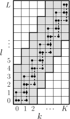
Figure 1: In the table of pairs $(k,l)$, the shaded cells correspond to balanced pairs, and the $K$-biased (dashed) and $L$-biased (dotted) walks are shown.

Definition 6.5

A pair of integers $(k,l)$ with $k\leq K$ and $l\leq L$ is said to be balanced if it satisfies

$$l\cdot\frac{K}{L}-2~{}\leq~{}k~{}\leq~{}l\cdot\frac{K}{L}+2.$$ (7)

Intuitively, in a set corresponding to a balanced pair, the numbers of elements from $R$ and $\bar{R}$ are proportional to the sizes of the two sets (see Figure 1).

Lemma 6.6

Suppose that $m\leq n$ elements are selected independently with probability $q\in[\frac{1}{n},\frac{n-1}{n}]$ each, and let $X$ denote the total number of selected elements. Then for any integer $x\in[0,m-1]$,

$$\frac{1}{n^{2}}~{}~{}\leq~{}~{}\frac{\Pr[X=x+1]}{\Pr[X=x]}~{}~{}\leq~{}~{}n^{2}.$$

Proof.

$$\frac{\Pr[X=x+1]}{\Pr[X=x]}~{}=~{}\frac{{m\choose x+1}~{}q^{x+1}~{}(1-q)^{m-x-1}}{{m\choose x}~{}q^{x}~{}(1-q)^{m-x}}~{}=~{}\frac{(m-x)~{}q}{(x+1)(1-q)},$$

with the minimum value of $1/m(n-1)\geq 1/n^{2}$ achieved at $x=m-1$ and $q=\frac{1}{n}$, and the maximum value of $m(n-1)\leq n^{2}$ achieved at $x=0$ and $q=\frac{n-1}{n}$. ∎

Lemma 6.7

If Algorithm 6 reaches step 4, then with probability at least $p$, for all balanced $(k_{1},l_{1})$ and $(k_{2},l_{2})$ such that $k_{1}+l_{1}=k_{2}+l_{2}$, it holds that $f(k_{1},l_{1})=f(k_{2},l_{2})$. In other words, for all balanced pairs $(k,l)$, the value of $f(k,l)$ depends only on $k+l$.

Proof.

The lemma follows if we show that with probability at least $p$, for each balanced $(k,l)$ with $k+l<n$, the algorithm samples at least one set $S$ corresponding to $(k,l)$. This is because the algorithm verifies that the function value for the sets that it samples depends only on the set size.

So consider a specific balanced pair $(k,l)$ and one random set $S$ generated by the iteration $i=k+l$ of step 2 of the algorithm. The probability of sampling each element in this iteration is $q=\frac{i}{n}=\frac{k+l}{K+L}$. Using (7) and its equivalent $(k-2)L/K\leq l\leq(k+2)L/K$, we see that this probability satisfies the following:

$$\frac{k}{K}-\frac{2L}{Kn}~{}\leq~{}q~{}\leq~{}\frac{k}{K}+\frac{2L}{Kn}~{}~{}~{}{\rm and}~{}~{}~{}\frac{l}{L}-\frac{2}{n}~{}\leq~{}q~{}\leq~{}\frac{l}{L}+\frac{2}{n}.$$

So the expected value of $|S\cap R|$ is $qK\in[k-2L/n,k+2L/n]\subseteq[k-2,k+2]$. Similarly, the expected value of $|S\cap\bar{R}|$ is $qL\in[l-2,l+2]$. Let $\mu_{k}$ be the most likely number of sampled elements when independently sampling $K$ elements with probability $q$ each. Then $\mu_{k}$ is equal to either $\lfloor qK\rfloor$ or $\lceil qK\rceil$. From above considerations and because $k$ is an integer, we have that $\mu_{k}\in[k-2,k+2]$. Now, since $\mu_{k}$ is the most likely value, we know that $\Pr[|S\cap R|=\mu_{k}]\geq 1/(K+1)\geq 1/n$. By Lemma 6.6 (with $m=K$),

$$\Pr[|S\cap R|=k]~{}\geq~{}\Pr[|S\cap R|=\mu_{k}]\cdot n^{-2\cdot|k-\mu_{k}|}~{}\geq~{}n^{-5}.$$

We similarly define $\mu_{l}$, observe that $\mu_{l}\in[l-2,l+2]$, and conclude that $\Pr[|S\cap\bar{R}|=l]\geq n^{-5}$. Since the two events are independent, the probability that both of them occur, and thus that $S$ corresponds to $(k,l)$, is at least $n^{-10}$.

We observe that for any $i$, there are at most four balanced pairs $(k,l)$ such that $k+l=i$. This is because if some pair $(k,l)$ satisfies (7), then the pair $(k-4,l+4)$ doesn’t satisfy it:

$$k-4~{}\leq~{}\left(l\frac{K}{L}+2\right)-4~{}=~{}l\frac{K}{L}-2~{}<~{}(l+4)\frac{K}{L}-2.$$

So there is a total of at most $4n$ pairs $(k,l)$ for which we would like the algorithm to sample their corresponding sets. Since the number of trials for each value of $k+l$ is $n^{10}\ln\left(\frac{4n}{1-p}\right)$, the probability that a set corresponding to any particular pair $(k,l)$ is not sampled is at most

$$\left(1-n^{-10}\right)^{n^{10}\ln\left(\frac{4n}{1-p}\right)}~{}\leq~{}e^{-\ln\left(\frac{4n}{1-p}\right)}~{}=~{}\frac{1-p}{4n}.$$

Since there are at most $4n$ pairs of interest, by union bound we have that the probability that at least one of them remains unsampled is at most $(1-p)$. ∎

Suppose the condition in Lemma 6.7 holds. Let us define a function $F(i)$ to be equal to $f(k,l)$ such that $k+l=i$ and $(k,l)$ is balanced. $F(i)$ is defined for all $i\in\{0,...,n\}$, since for any such $i$ there is at least one balanced pair $(k,l)$ with $k+l=i$.

Lemma 6.8

$F(i)$ is a non-decreasing concave function.

Proof.

Let $\Delta(i)=F(i+1)-F(i)$. It suffices to show that the sequence of increments $\Delta(i)$ is non-negative and non-increasing. For any $i$, we define a pair $(k_{i},l_{i})=\left(\left\lfloor\frac{iK}{n}\right\rfloor,\left\lceil\frac{iL}{n}\right\rceil\right)$. It can be verified that all pairs $(k_{i},l_{i})$ as well as $(k_{i}+1,l_{i})$ are balanced. Furthermore, $k_{i}+l_{i}=i$ (and consequently $k_{i}+1+l_{i}=i+1$), so that $f(k_{i}+1,l_{i})-f(k_{i},l_{i})=\Delta(i)$. Also, both $\{k_{i}\}$ and $\{l_{i}\}$ are non-decreasing sequences. The decreasing marginal values of the submodular function $f$ imply that $\Delta(i+1)=f(k_{i+1}+1,l_{i+1})-f(k_{i+1},l_{i+1})\leq f(k_{i}+1,l_{i})-f(k_{i},l_{i})=\Delta(i)$, showing that $\Delta(i)$’s are non-increasing. The monotonicity of $f$ implies that they are also non-negative. ∎

We next define two sequences of pairs, $(k^{K}_{i},l^{K}_{i})$ and $(k^{L}_{i},l^{L}_{i})$, ranging from $i=0$ to $i=n$, which we call the $K$-biased sequence (or walk) and the $L$-biased sequence, respectively (see Figure 1). The properties of these two sequences will be used in the remainder of the proof. The definitions are inductive, with both sequences starting at $(0,0)$.

$$(k^{K}_{i+1},~{}l^{K}_{i+1}) = \begin{cases}(k^{K}_{i}+1,~{}l^{K}_{i})&{\rm if}~{}~{}k^{K}_{i}\leq l^{K}_{i}\cdot\frac{K}{L}\\ (k^{K}_{i},~{}l^{K}_{i}+1)&{\rm if}~{}~{}k^{K}_{i}>l^{K}_{i}\cdot\frac{K}{L}\end{cases}$$

$$(k^{L}_{i+1},~{}l^{L}_{i+1}) = \begin{cases}(k^{L}_{i}+1,~{}l^{L}_{i})&{\rm if}~{}~{}k^{L}_{i}<l^{L}_{i}\cdot\frac{K}{L}\\ (k^{L}_{i},~{}l^{L}_{i}+1)&{\rm if}~{}~{}k^{L}_{i}\geq l^{L}_{i}\cdot\frac{K}{L}\end{cases}$$

Let us call the change from $(k_{i},l_{i})$ to $(k_{i+1},l_{i+1})$ in either of the two sequences a $K$-step if the first component of the pair increases by one, and an $L$-step if the second component increases. The only difference between the two sequences is that when equality $k=l\cdot K/L$ holds, we take a $K$-step in the case of the $K$-biased sequence, and an $L$-step in the case of the $L$-biased sequence. For both sequences it holds that $k^{K}_{i}+l^{K}_{i}=k^{L}_{i}+l^{L}_{i}=i$,  $k^{K}_{i}$ and $k^{L}_{i}$ range between $0$ and $K$, and $l^{K}_{i}$ and $l^{L}_{i}$ range between $0$ and $L$.

Lemma 6.9

All pairs in the $K$-biased and $L$-biased sequences are balanced.

Proof.

The proof is by induction, and it is the same for both sequences, so we denote either sequence by $(k_{i},l_{i})$. The first pair $(0,0)$ is balanced. Now we assume that the pair $(k_{i},l_{i})$ is balanced, and would like to show that the pair $(k_{i+1},l_{i+1})$ is also balanced. Suppose $(k_{i+1},l_{i+1})=(k_{i}+1,l_{i})$. Then it must be that $k_{i}\leq l_{i}\cdot\frac{K}{L}$. Then

$$l_{i}\cdot\frac{K}{L}-2~{}\leq~{}k_{i}~{}\leq~{}~{}k_{i}+1~{}~{}\leq~{}l_{i}\cdot\frac{K}{L}+1.$$

If $(k_{i+1},l_{i+1})=(k_{i},l_{i}+1)$, then it must be that $k_{i}\geq l_{i}\cdot\frac{K}{L}$. Then

$$(l_{i}+1)\cdot\frac{K}{L}-2~{}\leq~{}l_{i}\cdot\frac{K}{L}~{}\leq~{}~{}k_{i}~{}~{}\leq~{}l_{i}\cdot\frac{K}{L}+2~{}\leq~{}(l_{i}+1)\cdot\frac{K}{L}+2,$$

with the leftmost inequality following because $K/L\leq 1$. ∎

Lemma 6.10

In the $K$-biased sequence, every $K$-step is followed by at most $\left\lceil\frac{L}{K}\right\rceil$ $L$-steps. In the $L$-biased sequence, every $L$-step is followed by at most one $K$-step.

Proof.

Suppose that the $K$-biased sequence, after some point $(k,l)$, takes one $K$-step followed by $\left\lceil\frac{L}{K}\right\rceil$ $L$-steps, reaching the point $(k+1,l+\left\lceil\frac{L}{K}\right\rceil)$. Since the step after $(k,l)$ is a $K$-step, it must be that $k\leq lK/L$. So

$$\left(l+\left\lceil\frac{L}{K}\right\rceil\right)\cdot\frac{K}{L}~{}\geq~{}l\cdot\frac{K}{L}+1~{}\geq~{}k+1,$$

which means that the next step in the $K$-biased sequence will be a $K$-step.

Similarly, for the $L$-biased walk, suppose that from some point $(k,l)$, the sequence takes an $L$-step, followed by a $K$-step, reaching the point $(k+1,l+1)$. Then $k\geq lK/L$ implies that

$$(l+1)\cdot\frac{K}{L}~{}=~{}l\cdot\frac{K}{L}+\frac{K}{L}~{}\leq~{}l\cdot\frac{K}{L}+1~{}\leq~{}k+1,$$

and thus the next step is an $L$-step. ∎

Proof of Lemma 6.4..

To lower-bound the value of $f(k,0)$, we consider the $K$-biased walk from $(0,0)$ to a point $(k,l^{\prime})$ which is the last point before the $K$-step to $(k+1,\cdot)$. We let $f(k,0)=F(0)+\sum_{j=1}^{k}\delta(j)$, where $\delta(j)=f(j,0)-f(j-1,0)$. For each $K$-step in the $K$-biased walk, where $k^{K}_{i-1}=j-1$ and $k^{K}_{i}=j$, let $\Delta^{K}(j)=f(k^{K}_{i},l^{K}_{i})-f(k^{K}_{i-1},l^{K}_{i-1})=f(j,l^{K}_{i})-f(j-1,l^{K}_{i-1})$. By submodularity of $f$ it follows that $\Delta^{K}(j)\leq\delta(j)$.

We claim that $\sum_{j=1}^{k}\Delta^{K}(j)\geq[f(k,l^{\prime})-F(0)]/(1+\left\lceil\frac{L}{K}\right\rceil)$. In other words, at least $1/(1+\left\lceil\frac{L}{K}\right\rceil)$ fraction of the increase in $F(\cdot)$, as we proceed in the $K$-biased walk, is due to the $K$-steps. This follows from several observations. First, the $K$-biased walk starts with a $K$-step. Second, by Lemma 6.10, each $K$-step is followed by no more than $\left\lceil\frac{L}{K}\right\rceil$ $L$-steps. And third, $\Delta^{K}(j)$ is a decreasing sequence (by concavity of $F$).

Further, by concavity of $F$, we have that $f(k,l^{\prime})\geq\frac{k+l^{\prime}}{n}F(n)$. By definition of $l^{\prime}$, we have $l^{\prime}\geq kL/K$. Also, $1+\left\lceil\frac{L}{K}\right\rceil\leq 2(L/K+1)$. Putting everything together, we have

$$f(k,0) = F(0)+\sum_{j=1}^{k}\delta(j)~{}\geq~{}F(0)+\sum_{j=1}^{k}\Delta^{K}(j)~{}\geq~{}F(0)+\frac{f(k,l^{\prime})-F(0)}{1+\left\lceil\frac{L}{K}\right\rceil}~{}\geq~{}\frac{f(k,l^{\prime})}{1+\left\lceil\frac{L}{K}\right\rceil}$$

$$\geq \frac{k+l^{\prime}}{n}\frac{F(n)}{2(L/K+1)}~{}\geq~{}\frac{k(L/K+1)}{n}\frac{F(n)}{2(L/K+1)}~{}=~{}\frac{k}{2n}F(n)$$

To bound $f(0,l)$, we consider the $L$-biased walk from $(0,0)$ to $(k^{\prime},l)$ for some $k^{\prime}$. Because of concavity of $F$, the $L$-steps in the walk account for at least half the increase in $f$, yielding $f(0,l)\geq\frac{1}{2}f(k^{\prime},l)$. Also, $f(k^{\prime},l)\geq\frac{k^{\prime}+l}{n}F(n)\geq\frac{l}{n}F(n)$. So we get that $f(0,l)\geq\frac{l}{2n}F(n)$. ∎

7 Acknowledgements

We thank Mark Sandler for his help with some of the calculations and Satoru Iwata for useful discussions.

References

- [1] S. Arora, E. Hazan, and S. Kale. approximation to sparsest cut in time. In Proc. 45th IEEE Symp. on Foundations of Computer Science, pages 238–247, 2004.
- [2] S. Arora, S. Rao, and U. Vazirani. Expander flows, geometric embeddings and graph partitioning. In Proc. 36th ACM Symp. on Theory of Computing, 2004.
- [3] G. Calinescu, C. Chekuri, M. Pal, and J. Vondrak. Maximizing a submodular set function subject to a matroid constraint. SIAM J. Comput. To appear in STOC 2008 special issue.
- [4] G. Calinescu and A. Zelikovsky. The polymatroid Steiner problems. J. Comb. Optim., 9(3):281–294, 2005.
- [5] C. Chekuri and M. Pal. A recursive greedy algorithm for walks in directed graphs. In Proc. 46th IEEE Symp. on Foundations of Computer Science, pages 245–253, 2005.
- [6] T. Cormen, C. Leiserson, R. Rivest, and C. Stein. Introduction to Algorithms. MIT Press, second edition, 2001.
- [7] W.H. Cunningham. Minimum cuts, modular functions, and matroid polyhedra. Networks, 15:205–215, 1985.
- [8] U. Feige, V. Mirrokni, and J. Vondrak. Maximizing non-monotone submodular functions. In Proc. 48th IEEE Symp. on Foundations of Computer Science, 2007.
- [9] L. Fleischer and S. Iwata. A push-relabel framework for submodular function minimization and applications to parametric optimization. Discrete Appl. Math., 131(2):311–322, 2003.
- [10] S. Fujishige. Polymatroid dependence structure of a set of random variables. Info. and Control, 39:55–72, 1978.
- [11] G.V. Gens and E.V. Levner. Computational complexity of approximation algorithms for combinatorial problems. In Proc. 8th Intl. Symp. on Math. Foundations of Comput. Sci. Lecture Notes in Comput. Sci. 74, Springer-Verlag, 1979.
- [12] G. Goel, C. Karande, P. Tripathi, and L. Wang. Approximability of combinatorial problems with multi-agent submodular cost functions. In Proc. 50th IEEE Symp. on Foundations of Computer Science, 2009.
- [13] M. Goemans, N. Harvey, S. Iwata, and V. Mirrokni. Approximating submodular functions everywhere. In Proc. 20th ACM Symp. on Discrete Algorithms, 2009.
- [14] M. Goemans, N. Harvey, R. Kleinberg, and V. Mirrokni. Unpublished manuscript.
- [15] M. Grötschel, L. Lovász, and A. Schrijver. The ellipsoid method and its consequences in combinatorial optimization. Combinatorica, 1:169–197, 1981.
- [16] M. Grötschel, L. Lovász, and A. Schrijver. Geometric Algorithms and Combinatorial Optimization. Springer-Verlag, 1988.
- [17] A. Hayrapetyan, D. Kempe, M. Pal, and Z. Svitkina. Unbalanced graph cuts. In Proc. 13th European Symposium on Algorithms, 2005.
- [18] A. Hayrapetyan, C. Swamy, and E. Tardos. Network design for information networks. In Proc. 16th ACM Symp. on Discrete Algorithms, pages 933–942, 2005.
- [19] D. S. Hochbaum and D. B. Shmoys. Using dual approximation algorithms for scheduling problems: theoretical and practical results. J. ACM, 34:144–162, 1987.
- [20] S. Iwata. A faster scaling algorithm for minimizing submodular functions. SIAM J. Comput., 32:833–840, 2003.
- [21] S. Iwata. Submodular function minimization. Math. Programming, 112:45–64, 2008.
- [22] S. Iwata, L. Fleischer, and S. Fujishige. A combinatorial strongly polynomial algorithm for minimizing submodular functions. J. ACM, 48(4):761–777, 2001.
- [23] S. Iwata and K. Nagano. Submodular function minimization under covering constraints. In Proc. 50th IEEE Symp. on Foundations of Computer Science, 2009.
- [24] S. Iwata and J. B. Orlin. A simple combinatorial algorithm for submodular function minimization. In Proc. 20th ACM Symp. on Discrete Algorithms, 2009.
- [25] A. Kulik, H. Shachnai, and T. Tamir. Maximizing submodular set functions subject to multiple linear constraints. In Proc. 20th ACM Symp. on Discrete Algorithms, 2009.
- [26] J. Lee, V. Mirrokni, V. Nagarajan, and M. Sviridenko. Non-monotone submodular maximization under matroid and knapsack constraints. In Proc. 41th ACM Symp. on Theory of Computing, 2009.
- [27] J. Lee, M. Sviridenko, and J. Vondrak. Submodular maximization over multiple matroids via generalized exchange properties. In Proc. 12th APPROX, 2009.
- [28] F.T. Leighton and S. Rao. Multicommodity max-flow min-cut theorems and their use in designing approximation algorithms. Journal of the ACM, 46, 1999.
- [29] J. K. Lenstra, D. B. Shmoys, and E. Tardos. Approximation algorithms for scheduling unrelated parallel machines. Math. Programming, 46:259–271, 1990.
- [30] R. Motwani and P. Raghavan. Randomized Algorithms. Cambridge University Press, 1990.
- [31] G. Nemhauser, L. Wolsey, and M. Fisher. An analysis of the approximations for maximizing submodular set functions. Math. Program., 14:265–294, 1978.
- [32] J. B. Orlin. A faster strongly polynomial time algorithm for submodular function minimization. Math. Programming. To appear.
- [33] M. Queyranne. Minimizing symmetric submodular functions. Math. Programming, 82:3–12, 1998.
- [34] H. Räcke. Optimal hierarchical decompositions for congestion minimization in networks. In Proc. 40th ACM Symp. on Theory of Computing, pages 255–263, 2008.
- [35] A. Schrijver. A combinatorial algorithm minimizing submodular functions in strongly polynomial time. J. of Combinatorial Theory, Ser. B, 80(2):346–355, 2000.
- [36] M. Sviridenko. A note on maximizing a submodular set function subject to a knapsack constraint. Oper. Res. Lett., 32(1):41–43, 2004.
- [37] Z. Svitkina and E. Tardos. Min-max multiway cut. In Proc. 7th APPROX, pages 207–218, 2004.
- [38] Z. Svitkina and E. Tardos. Facility location with hierarchical facility costs. ACM Transactions on Algorithms, 6(2), 2010.
- [39] C. Swamy, Y. Sharma, and D. Williamson. Approximation algorithms for prize collecting steiner forest problems with submodular penalty functions. In Proc. 18th ACM Symp. on Discrete Algorithms, 2007.
- [40] J. Vondrak. Symmetry and approximability of submodular maximization problems. In Proc. 50th IEEE Symp. on Foundations of Computer Science, 2009.
- [41] L. A. Wolsey. An analysis of the greedy algorithm for the submodular set covering problem. Combinatorica, 2(4):385–393, 1982.
- [42] L. Zhao, H. Nagamochi, and T. Ibaraki. Greedy splitting algorithms for approximating multiway partition problems. Math. Program., 102(1):167–183, 2005.