Strong Convergence towards homogeneous cooling states for dissipative Maxwell models

Abstract

We show the propagation of regularity, uniformly in time, for the scaled solutions of the inelastic Maxwell model for small inelasticity. This result together with the weak convergence towards the homogenous cooling state present in the literature implies the strong convergence in Sobolev norms and in the $L^{1}$ norm towards it depending on the regularity of the initial data. The strategy of the proof is based on a precise control of the growth of the Fisher information for the inelastic Boltzmann equation. Moreover, as an application we obtain a bound in the $L^{1}$ distance between the homogeneous cooling state and the corresponding Maxwellian distribution vanishing as the inelasticity goes to zero.

Mathematics Subject Classification Numbers: 82C40, 35B40

1 Introduction

This paper concerns the regularity properties of solutions of the spatially homogeneous Boltzmann equation for Maxwellian molecules in ${\mathord{\mathbb{R}}}^{3}$ with inelastic collisions, introduced in [5]. This equation describes the evolution of the distribution of the velocities in a collection of particles as they interact through inelastic binary collisions. Let $f(v,t)$ be the probability density for the velocity of a particle chosen randomly from the collection at time $t$. Let $\varphi$ be any bounded and continuous function on ${\mathord{\mathbb{R}}}^{3}$. Then the equation under investigation is given, in weak form, by

$$\frac{{\rm d}}{{\rm d}t}\langle f,\varphi\rangle=\langle Q_{e}(f,f),\varphi\rangle$$ (1.1)

where $\langle f,\varphi\rangle$ denotes $\int_{{\mathord{\mathbb{R}}}^{3}}f(v,t)\varphi(v){\rm d}v$, and where

$$\langle Q_{e}(f,f),\varphi\rangle=\frac{1}{4\pi}\int_{{\mathord{\mathbb{R}}}^{3}}\int_{{\mathord{\mathbb{R}}}^{3}}\int_{S^{2}}\widetilde{B}\left(n\cdot\frac{v-w}{|v-w|}\right)f(v)f(w)[\varphi(v^{\prime})-\varphi(v)]\,{\rm d}n\,{\rm d}v\,{\rm d}w$$ (1.2)

where $n$ is a unit vector in $S^{2}$, ${\rm d}n$ is the uniform measure on $S^{2}$ with total mass $4\pi$, with $v^{\prime}$ the post collisional velocity given by

$$v^{\prime}=v-\frac{1+e}{2}((v-w)\cdot n)n\ ,$$ (1.3)

with $0\leq e\leq 1$, and where $\widetilde{B}$ is a positive, integrable even function on $[-1,1]$. Because of the integrability of $\widetilde{B}$, we can separate the collision operator in the gain and loss terms, $Q_{e}(f,f):=Q^{+}_{e}(f,f)-Q^{-}_{e}(f,f)$ with

$$Q^{-}_{e}(f,f):=\left(\int_{S^{2}}\widetilde{B}\left(n\cdot\frac{v-w}{|v-w|}\right)\,{\rm d}n\right)f=\left(\frac{1}{2}\int_{-1}^{1}\widetilde{B}(s)\,ds\right)f.$$

The function $\widetilde{B}$ gives the rate at which the various kinematically possible collisions happen, and the tilde is present because later on we shall also consider another rate function $B$ corresponding to another parameterization of the kinematically possible collisions.

The parameter $e$ is the restitution coefficient. For $e<1$, the collisions are inelastic, and energy is dissipated in each collision. In this case, the collisions are not reversible. This is a crucial difference with the elastic theory in which there is a complete time reversal symmetry between the pre and post collisional velocities. It is for this reason that we have written (1.1) in weak form, and not because of any difficulty in constructing strong solutions: It is just that to write the equation down in strong form, we need a parameterization of the possible pairs of precollisional velocities $(v^{*},w^{*})$ that can result in the pair of post collisional velocities $(v,w)$. We have detailed the strong formulation in the different parameterizations in the Appendix, see [5, 18] for particular cases, but for the purposes of the introduction, the weak form specifies the equation under consideration well enough for us to proceed with the description of the particular issues with which we are concerned, and the results we obtain.

The reason we require $\widetilde{B}$ to be even is that the post collisional velocity $v^{\prime}$ defined in (1.3) depends on $n$ quadratically, and thus is unchanged under the substitution $n\to-n$. For this reason, we may freely assume $\widetilde{B}$ to be even, and we do so in what follows.

The first thing to notice about the equation is that the first moment of $f$ is conserved. Indeed, for any $a\in{\mathord{\mathbb{R}}}^{3}$, let $\varphi(v)=a\cdot v$. Then we have from (1.1) and (1.3) that

$$\frac{{\rm d}}{{\rm d}t}\langle f,\varphi\rangle = -\frac{1+e}{8\pi}\int_{{\mathord{\mathbb{R}}}^{3}}\int_{{\mathord{\mathbb{R}}}^{3}}\int_{S^{2}}\widetilde{B}\left(n\cdot\frac{v-w}{|v-w|}\right)f(v)f(w)[((v-w)\cdot n)(a\cdot n)]{\rm d}v{\rm d}w{\rm d}n$$

$$= -\frac{1+e}{4}\left[\int_{-1}^{1}s^{2}\widetilde{B}(s){\rm d}s\right]\int_{{\mathord{\mathbb{R}}}^{3}}\int_{{\mathord{\mathbb{R}}}^{3}}f(v)f(w)a\cdot(v-w){\rm d}v{\rm d}w=0\ .$$

Indeed, as detailed in the appendix, the companion formula to (1.3), giving the other post collisional velocity $w^{\prime}$, is

$$w^{\prime}=w+\frac{1+e}{2}((v-w)\cdot n)n\ .$$

Thus, in each individual collision $(v,w)\to(v^{\prime},w^{\prime})$, the total momentum $v+w$ is conserved, and this certainly ensures that the first moment of $f$ is conserved. In any case, on account of the computation just made, we may as well assume that our initial data $f_{0}$ satisfies

$$\int_{{\mathord{\mathbb{R}}}^{3}}vf_{0}(v)\,{\rm d}v=0\ .$$

Then of course we shall have

$$\int_{{\mathord{\mathbb{R}}}^{3}}vf(v,t)\,{\rm d}v=0$$ (1.4)

for all $t\geq 0$. While momentum is conserved, energy is dissipated, as we have indicated above. We now calculate the rate of this dissipation: Take $\varphi(v)=|v|^{2}$ and then note that from (1.3)

$$\varphi(v^{\prime})=|v|^{2}-(1+e)((v-w)\cdot n)(v\cdot n)+\frac{(1+e)^{2}}{4}((v-w)\cdot n)^{2}\ .$$

In this case, using the abreviated notation $u=v-w$, we have

$$\frac{{\rm d}}{{\rm d}t}\langle f,\varphi\rangle\!\! = \!\!\frac{1}{4\pi}\int_{{\mathord{\mathbb{R}}}^{3}}\!\int_{{\mathord{\mathbb{R}}}^{3}}\!\int_{S^{2}}\!\widetilde{B}\left(n\cdot\frac{u}{|u|}\right)f(v)f(w)\left[\frac{(1+e)^{2}}{4}(u\cdot n)^{2}-(1+e)(u\cdot n)(v\cdot n)\right]{\rm d}v{\rm d}w{\rm d}n$$

$$= \left[\frac{1}{2}\int_{-1}^{1}s^{2}\widetilde{B}(s){\rm d}s\right]\int_{{\mathord{\mathbb{R}}}^{3}}\int_{{\mathord{\mathbb{R}}}^{3}}f(v)f(w)\left(\frac{(1+e)^{2}}{4}|u|^{2}-(1+e)u\cdot v\right){\rm d}v{\rm d}w$$

$$= -\left[\frac{1}{2}\int_{-1}^{1}s^{2}\widetilde{B}(s){\rm d}s\right]\frac{1-e^{2}}{2}\langle f,\varphi\rangle\ .$$

That is, with the positive constant $E$ defined by

$$E=\left[\frac{1}{2}\int_{-1}^{1}s^{2}\widetilde{B}(s){\rm d}s\right]\frac{1-e^{2}}{4}\ ,$$ (1.5)

we have every solution of (1.1) with initial data $f_{0}$ satisfying (1) satisfies

$$\frac{{\rm d}}{{\rm d}t}\int_{{\mathord{\mathbb{R}}}^{3}}|v|^{2}f(v,t){\rm d}v=-2E\int_{{\mathord{\mathbb{R}}}^{3}}|v|^{2}f(v,t){\rm d}v\ .$$ (1.6)

This implies that $f(v,t){\rm d}v$ tends to a point mass at $v=0$ as $t$ tends to infinity. It is natural to enquire into precise nature of this collapse to a point mass. In previous works [6, 9, 2, 7, 8, 10], it has been shown that if one rescales $f(v,t)$ to keep the variance (i.e., temperature) constant, then the rescaled density tends to a particular equilibrium state, known as the homogeneous cooling state. That is, if we define the probability density $g(v,t)$ by

$$g(v,t)={\rm e}^{-3Et}f\left({\rm e}^{-Et}v,t\right)\ ,$$ (1.7)

$$\int_{{\mathord{\mathbb{R}}}^{3}}|v|^{2}g(v,t){\rm d}v=\int_{{\mathord{\mathbb{R}}}^{3}}|v|^{2}g(v,0){\rm d}v=\int_{{\mathord{\mathbb{R}}}^{3}}|v|^{2}f_{0}(v){\rm d}v$$

for all $t$, and there is a density $g_{\infty}$ such that

$$\lim_{t\to\infty}g(v,t)=g_{\infty}(v)\ .$$ (1.8)

The convergence in (1.8), part of the so-called Ernst-Brito conjecture [16, 17, 6, 9], has so far been shown in certain weak norms that we shall introduce shortly, see [13] for a review and [9, 2] for the proofs. Our goal in this paper is to prove that $g(v,t)$ is regular in $v$, uniformly in $t$. This is reasonable to expect since it is was proved by Bobylev and Cercignani that $g_{\infty}(v)$ itself is quite regular [6, Theorem 7.1]. However, it is clear from the fact that $f(v,t){\rm d}v$ tends to a point mass that the norm of $f(\cdot,t)$ must diverge with $t$ in every norm that would imply smoothness of $f(\cdot,t)$. While the rescaling may well lower such norms, one needs very precise estimates on the loss of regularity to avoid having them overwhelm whatever one gains from the rescaling. Notice in particular that the rescaling does nothing to improve regularity.

To investigate the long time behavior of $g(v,t)$, we write down its evolution equation, which of course is obtained from (1.1) through (1.7). In working out the equation, we make use of the dilation invariance of the collision integral $Q_{e}(f,f)$: For any density $f$, test function $\varphi$ and any $\lambda>0$, define

$$f^{(\lambda)}(v)=\lambda^{3}f(\lambda v)\qquad{\rm and}\qquad\varphi^{(\lambda)}(v)=\varphi(v/\lambda)\ .$$ (1.9)

Then one easily sees from (1.2) that

$$\langle Q_{e}(f^{(\lambda)},f^{(\lambda)}),\varphi\rangle=\langle Q_{e}(f,f),\varphi^{(\lambda)}\rangle\ .$$ (1.10)

Then, for any test function $\varphi$,

$$\frac{{\rm d}}{{\rm d}t}\langle g,\varphi\rangle = \frac{{\rm d}}{{\rm d}t}\langle f,\varphi^{(\exp(-Et))}\rangle$$

$$= -E{\rm e}^{-Et}\langle f,v\cdot\left(\nabla\varphi\right)^{(\exp(-Et))}\rangle+\langle Q(f,f),\varphi^{(\exp(-Et))}\rangle$$

$$= -E\langle g,\left(v\cdot\nabla\varphi\right)\rangle+\langle Q(f,f),\varphi^{(\exp(-Et))}\rangle$$

$$= -E\langle g,\left(v\cdot\nabla\varphi\right)\rangle+\langle Q(g,g),\varphi\rangle$$

where we have used (1.10) in the last line. Thus, our evolution equation for $g$ is, in weak form,

$$\frac{{\rm d}}{{\rm d}t}\langle g,\varphi\rangle=-E\langle g,\left(v\cdot\nabla\varphi\right)\rangle+\langle Q(g,g),\varphi\rangle\ .$$ (1.11)

There are other ways, physically and mathematically different, to control the temperature/variance: If the particles are in contact with an appropriate heat bath, this will add a thermal regularization to the evolution equation for $f$. This thermal bath can be modelled by stochastic heating, i.e.,

$$\frac{\partial f}{\partial t}=Q_{e}(f,f)+\Delta_{v}f$$

or by a thermalized bath of particles, adding a linear Boltzmann type operator. In these two cases, global regularity estimates for solutions have been obtained, see [1, 13, 25]. However, as the first order anti–drift term in (1.11) does not induce a priori any regularization, the problem of proving global regularity estimate for solutions of (1.11) is more challenging.

The Fisher information plays a crucial role in our investigation of regularity. For any probability density $f$ on ${\mathord{\mathbb{R}}}^{3}$, the Fisher information, $I(f)$, is defined by

$$I(f)=4\int_{{\mathord{\mathbb{R}}}^{3}}|\nabla\sqrt{f(v)}|^{2}\,{\rm d}v=\int_{{\mathord{\mathbb{R}}}^{3}}|\nabla\ln f(v)|^{2}f(v)\,{\rm d}v$$

whenever the distributional gradient of $\sqrt{f}$ is square integrable, and it is defined to be infinite otherwise. It has been shown by Villani that in case $e=1$; i.e, for elastic collisions, the Fisher information is non increasing in time. This is a basic propagation of regularity result that is the starting point of our investigation of the inelastic case.

For solutions of (1.11), the Fisher information will not be bounded uniformly in time. Indeed, the Fisher information has simple scaling properties: If $f^{(\lambda)}$ is defined in terms of $f$ and $\lambda$ as in (1.9), one easily computes

$$I(f^{(\lambda)})=\lambda^{2}I(f)\ .$$ (1.12)

Therefore, with $g(v,t)$ defined in terms of $f(v,t)$ through the scaling relation (1.7), we have

$$I(g(\cdot,t))={\rm e}^{-2Et}I(f(\cdot,t))\ .$$ (1.13)

The exponentially decreasing factor ${\rm e}^{-2Et}$ is good, but notice from (1.5) that it depends only on $\widetilde{B}$ and the restitution coefficient $e$, and not on the initial data. For some initial data, $I(f(\cdot,t))$ will grow faster than this rate, and thus $I(g(\cdot,t))$ will grow exponentially. Nonetheless, we shall be able to prove that its growth is not too bad, at least for $e$ not too far from $1$.

1.1 THEOREM.

For any solution $g(v,t)$ of (1.11), we have a bound on the Fisher information

$$I(g(\cdot,t))\leq{\rm e}^{[(1-e)(2+e+15e^{2})/(8e^{3})-2E]t}I(g(\cdot,0))$$

where $E$ is the constant defined in (1.5). While the exponent is always positive, no matter how $\widetilde{B}$ is chosen, it does always vanish in the limit $e\to 1$.

Theorem 1.1 is proved in Section 2. Our main goal in the next part of the paper is to obtain a tiny uniform-in-time propagation of regularity result of the type:

1.2 THEOREM.

For any $0<\delta<1$, there is a computable positive constant $C$, such that for any solution $g$ of (1.11) corresponding to the initial value $f_{0}$ with unit mass, zero mean velocity, $|v|^{2+\alpha}f_{0}\in L^{1}({\mathord{\mathbb{R}}}^{3})$ with $0<\alpha<1$ and $I(f_{0})<\infty$, then

$${\|}|\eta|^{\delta}\hat{g}(\eta){\|}_{L^{\infty}({\mathord{\mathbb{R}}}^{3})}\leq C,$$ (1.14)

for all $t>0$, being $e$ close enough to 1.

This strategy precisely coincides with the open problem left in [13] for strong convergence to homogeneous cooling states and applied in the case of the thermalized bath of particles, adding a linear Boltzmann type operator, see [13, Subsubsection 7.2.4].

To prove the convergence in strong norms towards the homogeneous cooling state, we will need more; we will need the propagation of regularity in Sobolev spaces of high degree:

$${\|}g{\|}_{\dot{H}^{r}({\mathord{\mathbb{R}}}^{3})}^{2}=\int_{{\mathord{\mathbb{R}}}^{3}}|\eta|^{2r}|\hat{g}(\eta)|^{2}\,d\eta$$ (1.15)

with $r>0$. However, there is a well-developed machinery [12, 13] for showing that whenever the equation propagates a tiny degree of regularity, this implies the equation propagates regularity of any degree. Therefore, the main problem to be solved is to prove (1.14), uniformly in time for which there are no standard arguments.

Then, using the regularity in high Sobolev spaces, we can parley the weak convergence in (1.8) into convergence in all Sobolev norms, Theorem 3.9, and strong $L^{1}$ convergence at an explicit exponential rate for a certain class of initial data. This is the objective of Section 3 and the main result is summarized as:

1.3 THEOREM.

Given the solution $g$ of (1.11) corresponding to the initial probability distribution function $f_{0}\in\dot{H}^{r}({\mathord{\mathbb{R}}}^{3})$, with $r>0$, of zero mean velocity such that $|v|^{4}f_{0}\in L^{1}({\mathord{\mathbb{R}}}^{3})$ and $I(f_{0})<\infty$. Then, for $e$ close to 1, the solution $g(t,v)\!$ of (1.11) converges strongly in $L^{1}$ with an exponential rate towards the homogenous cooling state, i.e., there exist positive constants $C$ and $\gamma^{\prime}$ explicitly computable such that

$${\|}g(t)-g_{\infty}{\|}_{L^{1}({\mathord{\mathbb{R}}}^{3})}\leq C\,{\rm e}^{-\gamma^{\prime}t}$$

for all $t>0$.

Finally, we can study the small inelasticity limit of the sequence of homogeneous cooling states showing an $L^{1}$ convergence towards the Maxwellian distribution with zero mean velocity and temperature fixed by the initial data as $e\to 1$ with an explicit speed in terms of the inelasticity parameter. Section 4 is devoted to this small inelasticity limit in strong norms. Finally, as announced above, the appendix is aimed at a detailed description of the relations between the different parameterizations of the collision mechanism that we have written for non necessarily Maxwellian type collision kernels.

2 Fisher Information bounds

Villani [23] has proved that for Maxwellian molecules and elastic collisions, the Fisher information does not increase. A special case of this, namely with $\widetilde{B}$ constant, had been treated earlier by Carlen and Carvalho using the reflection parameterization [11]. Villani’s analysis is based on the $\sigma$ representation, and has the advantage it allows an arbitrary rate function $B$. All of these results use the strong formulation of the collision operator, the passage from the weak form to the strong form is merely a complicated change of variables that we detail in the appendix. The main formulas we will use in this section are related to the strong formulation in the $\sigma$-representation,

$$Q_{e}^{+}(f,f)(v)=\frac{1}{4\pi}\int_{{\mathord{\mathbb{R}}}^{3}}\int_{S^{2}}f(v^{*})f(w^{*})B_{e}^{+}(k\cdot\sigma){\rm d}\sigma{\rm d}w$$

with $u=v-w$, $k=u/|u|$,

$$B_{e}^{+}(s)=B\left(\frac{(1+e^{2})s-(1-e^{2})}{(1+e^{2})-(1-e^{2})s}\right)\frac{\sqrt{2}}{\sqrt{{(1+e^{2})-(1-e^{2})s}}}\frac{1}{e}\qquad,\qquad B(s)=\frac{\widetilde{B}\left(\sqrt{(1-s)/2}\right)}{2\sqrt{(1-s)/2}}$$

and the precollisional velocities are given by

$$\begin{cases}v^{*}&=\ {\displaystyle\frac{v+w}{2}-\frac{1-e}{4e}(v-w)+\frac{1+e}{4e}|v-w|\sigma}\\[8.53581pt] w^{*}&=\ {\displaystyle\frac{v+w}{2}+\frac{1-e}{4e}(v-w)-\frac{1+e}{4e}|v-w|\sigma}\end{cases}\,.$$

The reader can understand now why we have avoided the strong formulation as long as we could. We emphasize that this operator coincides with the one defined in weak form below (1.2). Full details of the passage from one representation to the other are given in the appendix.

We now start to adapt Villani’s analysis to the inelastic case, and derive bounds on the growth of the Fisher information in terms of the restitution coefficient $e$. The crucial feature of these bounds on the growth is that they vanish as $e$ tends towards $1$. The main result of this section is:

2.1 THEOREM.

For all probability densities $f$ on ${\mathord{\mathbb{R}}}^{3}$,

$$I(Q_{e}^{+}(f,f))\leq\left[1+(1-e)\left(\frac{2+e+15e^{2}}{8e^{3}}\right)\right]\,I(f)\ ,$$ (2.1)

with the consequence that if $f(v,t)$ is a solution of (1.1), we have

$$I(f(\cdot,t))\leq{\rm e}^{[(1-e)(2+e+15e^{2})/(8e^{3})]t}I(f(\cdot,0))\ .$$ (2.2)

As an immediate consequence of this, we obtain the proof of Theorem 1.1:

Proof of Theorem 1.1: Consider any rescaled solution $g(v,t)$; i.e., any solution of (1.11). By (1.13), any solution $g(v,t)$ of (1.11) satisfies

$$I(g(\cdot,t))\leq{\rm e}^{[(1-e)(2+e+15e^{2})/(8e^{3})-2E]t}I(g(\cdot,0))\ .$$ (2.3)

where $E$ is given by (1.5). Notice that while $E$ depends on the particular choice of $\widetilde{B}$, for any choice we have

$$E\leq(1-e)\frac{1+e}{4}<\frac{1-e}{2}\ .$$

Therefore, for any $\widetilde{B}$, the exponent in (2.3) is at least

$$(1-e)\left(\frac{2+e+15e^{2}}{8e^{3}}-1\right)>0\ ,$$

for all $0\leq e<1$.∎

While the exponent in Theorem 1.1 is always positive, it does vanish in the elastic limit, and that is what we shall need in the next sections. We begin by recalling several results:

2.2 LEMMA.

[23, Lemma 1] Let $P_{k}$ denote the orthogonal projection onto the span of $k$, and let $P^{\perp}_{k}$ denote its orthogonal complement. Then for any differentiable rate function $B$,

$$\nabla_{v}\left[B(k\cdot\sigma)\right]=\frac{1}{|u|}B^{\prime}(k\cdot\sigma)P^{\perp}_{k}\sigma\ ,$$

where $B^{\prime}$ is the derivative of $B$.

The proof of this Lemma is an elementary computation. Applying it with $B=B_{e}^{+}$, and defining $F(v,w,\sigma)=f(v^{*})f(w^{*})$ we have

$$\nabla_{v}Q_{e}^{+}(f,f)=\frac{1}{4\pi}\int_{S^{2}}\!\int_{{\mathord{\mathbb{R}}}^{3}}\!\!\left[\frac{1}{|u|}(B_{e}^{+})^{\prime}(k\cdot\sigma)P_{k}^{\perp}\sigma F(v,w,\sigma)+B_{e}^{+}(k\cdot\sigma)\nabla_{v}F(v,w,\sigma)\right]{\rm d}w{\rm d}\sigma\ .$$ (2.4)

The proof of the next Lemma is not so elementary, as done in [23], it is an ingenious integration by parts on the sphere. Later on, we will give a different proof of the formula resulting from this Lemma in a more direct way.

2.3 LEMMA.

[23, Lemma 2] Using the notation of the previous lemma and also defining the linear transformation $M_{\sigma,k}$ on ${\mathord{\mathbb{R}}}^{3}$ by

$$M_{\sigma,k}(x)=(k\cdot\sigma)x-(k\cdot x)\sigma\ ,$$

we have that for any smooth function $F(\sigma)$ on $S^{2}$,

$$\int_{S^{2}}B^{\prime}(k\cdot\sigma)P^{\perp}_{k}\sigma F(\sigma){\rm d}\sigma=\int_{S^{2}}B(\sigma\cdot k)M_{\sigma,k}\left[\nabla_{\sigma}F(\sigma)\right]{\rm d}\sigma\ .$$

Using this Lemma on (2.4) we obtain

$$\nabla_{v}Q_{e}^{+}(f,f)=\frac{1}{4\pi}\int_{S^{2}}\!\int_{{\mathord{\mathbb{R}}}^{3}}\!\!\left[\frac{1}{|u|}B_{e}^{+}(\sigma\cdot k)M_{\sigma,k}\left[\nabla_{\sigma}F(v,w,\sigma)\right]+B_{e}^{+}(k\cdot\sigma)\nabla_{v}F(v,w,\sigma)\right]{\rm d}w{\rm d}\sigma\ .$$ (2.5)

Next, using (A.36) to evaluate the Jacobians,

$$\nabla_{v}\left[f(v^{*})\right]=\left(\frac{\partial v^{*}}{\partial v}\right)(\nabla_{v}f)(v^{*})=\frac{3e-1}{4e}(\nabla_{v}f)(v^{*})+\frac{1+e}{4e}(\sigma\cdot\nabla_{v}f)(v^{*})k$$

and

$$\nabla_{v}\left[f(w^{*})\right]=\left(\frac{\partial w^{*}}{\partial v}\right)(\nabla_{v}f)(w^{*})=\frac{e+1}{4e}(\nabla_{v}f)(w^{*})-\frac{1+e}{4e}(\sigma\cdot\nabla_{v}f)(w^{*})k\,.$$

Also from (A.36),

$$\nabla_{\sigma}F(v,w,\sigma)=\frac{1+e}{4e}|u|\left[(\nabla_{v}f)(v^{*})f(w^{*})-f(v^{*})(\nabla_{v}f)(w^{*})\right]\ .$$

Therefore, if we define the linear transformation $P_{\sigma,k}$ on ${\mathord{\mathbb{R}}}^{3}$ by $P_{\sigma,k}(x)=(\sigma\cdot x)k+M_{\sigma,k}(x)$, we can rewrite (2.5) as

$$\nabla_{v}Q_{e}^{+}(f,f)=\frac{1}{4\pi}\int_{S^{2}}\int_{{\mathord{\mathbb{R}}}^{3}}B_{e}^{+}(\sigma\cdot k)G(v,w,\sigma){\rm d}\sigma{\rm d}w$$ (2.6)

where

$$G(v,w,\sigma)= \,\,\,\,\,\,\,\,f(w^{*})\left(\frac{3e-1}{4e}+\frac{1+e}{4e}P_{\sigma,k}\phantom{.}\right)\left[(\nabla_{v}f)(v^{*})\right]$$

$$+f(v^{*}\phantom{.})\left(\frac{1+e}{4e}\ -\ \frac{1+e}{4e}P_{\sigma,k}\right)\left[(\nabla_{v}f)(w^{*})\right]\ .$$ (2.7)

Before proceeding further, let us give a simple, direct proof of formula (2.7) making use of the Fourier transform instead of Lemma 2.3.

Proof of (2.6)-(2.7): We start by recalling the formula of the Fourier representation of $Q_{e}^{+}(f,f)$ obtained in [5], see previous works [3, 4] and [15, 13] for a review. It holds

$$\widehat{Q_{e}^{+}(f,f)}(\eta)=\frac{1}{4\pi}\int_{S^{2}}B(\tilde{\eta}\cdot\sigma)\hat{f}(t,\eta_{-})\hat{f}(t,\eta_{+})\,d\sigma$$ (2.8)

with $\tilde{\eta}=\eta/|\eta|$ and

$$\begin{array}[]{l}\displaystyle\eta_{-}=\frac{1+e}{4}(\eta-|\eta|\sigma),\vspace{0.3 cm}\\ \displaystyle\eta_{+}=\frac{3-e}{4}\,\eta+\frac{1+e}{4}\,|\eta|\sigma=\eta-\eta_{-}\,.\end{array}$$ (2.9)

Now, let us point out the following identity, left for the reader to check,

$$Z(\eta_{+},\eta_{-}):=\frac{3e-1}{4e}\eta_{+}+\frac{1+e}{4e}P_{\sigma,\tilde{\eta}}(\eta_{+})+\frac{1+e}{4e}\eta_{-}-\ \frac{1+e}{4e}P_{\sigma,\tilde{\eta}}(\eta_{-})=\eta+\frac{1-e^{2}}{4e}\left((\eta\cdot\sigma)\tilde{\eta}-|\eta|\sigma\right).$$

Now, multiplying both sides by $\frac{1}{4\pi}B(\tilde{\eta}\cdot\sigma)\hat{f}(t,\eta_{-})\hat{f}(t,\eta_{+})$ and integrating over the sphere, we get

$$\frac{1}{4\pi}\int_{S^{2}}B(\tilde{\eta}\cdot\sigma)\hat{f}(t,\eta_{-})\hat{f}(t,\eta_{+})Z(\eta_{+},\eta_{-})\,d\sigma=\eta\,\widehat{Q_{e}^{+}(f,f)}(\eta)=\widehat{\left[\nabla_{v}Q_{e}^{+}(f,f)\right]}(\eta)$$ (2.10)

since the integral of the last term is zero. In fact, since we are free to choose our coordinate system in the sphere, it is easy to see that

$$\int_{S^{2}}(\eta\cdot\sigma)\tilde{\eta}\,J(\eta,\sigma)\,d\sigma=\int_{S^{2}}|\eta|\sigma\,J(\eta,\sigma)\,d\sigma$$

for any function $J(\eta,\sigma)$. The desired formula (2.6)-(2.7) is just the inverse Fourier transform formula corresponding to (2.10). ∎

Now, starting from (2.7), we can define $H(v,w,\sigma)$ by

$$H(v,w,\sigma)= \,2\sqrt{f(w^{*})}\left(\frac{3e-1}{4e}+\frac{1+e}{4e}P_{\sigma,k}\phantom{.}\right)\left[(\nabla_{v}\sqrt{f})(v^{*})\right]$$

$$+2\sqrt{f(v^{*}\phantom{.})}\left(\frac{1+e}{4e}\ -\ \frac{1+e}{4e}P_{\sigma,k}\right)\left[(\nabla_{v}\sqrt{f})(w^{*})\right]\ ,$$

$$= \,\left[\frac{3e-1}{2e}\sqrt{f(w^{*})}(\nabla_{v}\sqrt{f})(v^{*})+\frac{1+e}{2e}\sqrt{f(v^{*}\phantom{.})}(\nabla_{v}\sqrt{f})(w^{*})\right]$$

$$+P_{\sigma,k}\left(\frac{1+e}{2e}\right)\left[\sqrt{f(w^{*})}(\nabla_{v}\sqrt{f})(v^{*})-\sqrt{f(v^{*}\phantom{.})}(\nabla_{v}\sqrt{f})(w^{*})\right]$$

$$= \,H_{1}(v,w,\sigma)+P_{\sigma,k}H_{2}(v,w,\sigma)\ ,$$ (2.11)

where the last line defines $H_{1}(v,w,\sigma)$ and $H_{2}(v,w,\sigma)$, and $G(v,w,\sigma)=\sqrt{f(v^{*})f(w^{*})}H(v,w,\sigma)$. Thus, we get

$$\nabla_{v}Q_{e}^{+}(f,f)=\frac{1}{4\pi}\int_{S^{2}}\int_{{\mathord{\mathbb{R}}}^{3}}B_{e}^{+}(\sigma\cdot k)\sqrt{f(v^{*})f(w^{*})}H(v,w,\sigma){\rm d}\sigma{\rm d}w\ .$$ (2.12)

Therefore, by the Schwarz inequality

$$|\nabla_{v}Q_{e}^{+}(f,f)(v)|\leq\left(Q_{e}^{+}(f,f)(v)\right)^{1/2}\left(\frac{1}{4\pi}\int_{S^{2}}\int_{{\mathord{\mathbb{R}}}^{3}}B_{e}^{+}(\sigma\cdot k)H^{2}(v,w,\sigma){\rm d}\sigma{\rm d}w\right)^{1/2}\ .$$ (2.13)

From here we obtain a bound of $I(Q_{e}^{+}(f,f))$: Squaring both sides, and integrating in $v$ we obtain

$$I(Q_{e}^{+}(f,f))\leq\frac{1}{4\pi}\int_{{\mathord{\mathbb{R}}}^{3}}\int_{{\mathord{\mathbb{R}}}^{3}}\int_{S^{2}}B_{e}^{+}(\sigma\cdot k)|H(v,w,\sigma)|^{2}{\rm d}\sigma{\rm d}w{\rm d}v\ .$$ (2.14)

It remains to estimate the integral on the right in terms of $I(f)$. This consists of the sum of three terms:

$$S_{1} =\frac{1}{4\pi}\int_{{\mathord{\mathbb{R}}}^{3}}\int_{{\mathord{\mathbb{R}}}^{3}}\int_{S^{2}}B_{e}^{+}(\sigma\cdot k)|H_{1}(v,w,\sigma)|^{2}{\rm d}\sigma{\rm d}w{\rm d}v$$

$$S_{2} =\frac{1}{4\pi}\int_{{\mathord{\mathbb{R}}}^{3}}\int_{{\mathord{\mathbb{R}}}^{3}}\int_{S^{2}}B_{e}^{+}(\sigma\cdot k)|P_{\sigma,k}H_{2}(v,w,\sigma)|^{2}{\rm d}\sigma{\rm d}w{\rm d}v$$ (2.15)

$$S_{3} =\frac{1}{4\pi}\int_{{\mathord{\mathbb{R}}}^{3}}\int_{{\mathord{\mathbb{R}}}^{3}}\int_{S^{2}}B_{e}^{+}(\sigma\cdot k)(H_{1}\cdot P_{\sigma,k}H_{2})(v,w,\sigma){\rm d}\sigma{\rm d}w{\rm d}v\ .$$

Summarizing the discussion so far, we have: For any probability density $f$ on ${\mathord{\mathbb{R}}}^{3}$, we have

$$I(Q_{e}^{+}(f,f))\leq S_{1}+S_{2}+2S_{3}\ ,$$

where the quantities on the right hand side are specified in (2). Our next lemma simplifies these expressions by a change of variables:

2.4 LEMMA.

For any probability density $f$ on ${\mathord{\mathbb{R}}}^{3}$, we have

$$S_{1} =\frac{1}{4\pi}\int_{{\mathord{\mathbb{R}}}^{3}}\int_{{\mathord{\mathbb{R}}}^{3}}\int_{S^{2}}B(\sigma\cdot k)|F_{1}(v,w)|^{2}{\rm d}\sigma{\rm d}w{\rm d}v$$

$$S_{2} =\frac{1}{4\pi}\int_{{\mathord{\mathbb{R}}}^{3}}\int_{{\mathord{\mathbb{R}}}^{3}}\int_{S^{2}}B(\sigma\cdot k)|P_{\sigma^{\prime},k^{\prime}}F_{2}(v,w)|^{2}{\rm d}\sigma{\rm d}w{\rm d}v$$ (2.16)

$$S_{3} =\frac{1}{4\pi}\int_{{\mathord{\mathbb{R}}}^{3}}\int_{{\mathord{\mathbb{R}}}^{3}}\int_{S^{2}}B(\sigma\cdot k)(F_{1}(v,w)\cdot P_{\sigma^{\prime},k^{\prime}}F_{2})(v,w){\rm d}\sigma{\rm d}w{\rm d}v$$

where

$$k^{\prime}=\frac{(1-e)k+(1+e)\sigma}{\sqrt{2(1+e^{2})+2(1-e^{2})k\cdot\sigma}}\ ,\qquad\sigma^{\prime}=\frac{(1+e)k+(1-e)\sigma}{\sqrt{2(1+e^{2})+2(1-e^{2})k\cdot\sigma}}\ ,$$ (2.17)

$$F_{1}(v,w)=\left(\frac{3e-1}{2e}\sqrt{f(w)}(\nabla\sqrt{f})(v)+\frac{1+e}{2e}\sqrt{f(v)}(\nabla\sqrt{f})(w)\right)$$ (2.18)

and

$$F_{2}(v,w)=\left(\frac{1+e}{2e}\right)\left(\sqrt{f(w)}(\nabla\sqrt{f})(v)-\sqrt{f(v)}(\nabla\sqrt{f})(w)\right)\ .$$ (2.19)

Proof: In the expressions in (2), we are integrating over post collisional variables. We use the change of variables Theorem A.1, which concerns the transformation $C_{s,e}(v,w,\sigma)\mapsto(v^{*},w^{*},\sigma^{*})$ from post to pre collisional variables under the “swapping map”; i.e., for the sigma representation. Consulting Theorem A.1 and the definition of $H_{1}$ and $H_{2}$ in (2.11), we see that each of the integrands above can be written out in the longer form appearing in Theorem A.1, e.g.,

$$|H_{1}(v,w,\sigma)|^{2}=K[(v^{*},w^{*},\sigma^{*}),(v,w,\sigma)]=K[C_{s,e}^{-1}(v,w,\sigma),(v,w,\sigma)]\ .$$

Theorem A.1 allows us to write this as an integral over

$$K[(v,w,\sigma),C_{s,e}(v,w,\sigma)]=K[(v,w,\sigma),(v^{\prime},w^{\prime},\sigma^{\prime})]\ .$$

Doing this for each of the three integrals in (2), we obtain the stated formulas. ∎

Define the matrix $A_{\sigma,k}$ by

$$A_{\sigma,k}=P_{\sigma^{\prime},k^{\prime}}-P_{k,\sigma}\ .$$

We shall now prove:

2.5 LEMMA.

For all $\sigma$, $k$ and $z$ in ${\mathord{\mathbb{R}}}^{3}$ such that $|\sigma|=|k|=1$,

$$|A_{\sigma,k}(z)|\leq 2\frac{1-e}{e}|z|\ .$$

In proving this Lemma, as well as for estimating $S_{2}$, we shall make use of the following lemma of Villani:

2.6 LEMMA.

[23, Lemma 4] For all $\sigma$, $k$ and $z$ in ${\mathord{\mathbb{R}}}^{3}$ such that $|\sigma|=|k|=1$,

$$|P_{\sigma,k}(z)|\leq|z|$$

with equality if and only if $\sigma$, $k$ and $z$ belong to the same plane.

Proof of Lemma 2.5:, considering the formulas for $k^{\prime}$ and $\sigma^{\prime}$ given in (A.25) and (A.26) respectively, notice that as $e\to 1$, we have $k^{\prime}\to\sigma$ and $\sigma^{\prime}\to k$, as we should, since in the elastic case, this is what the swapping map does. Therefore, using (A.25) and (A.26) we compute

$$k^{\prime}-\sigma=\frac{(1-e)k+(e+1-\sqrt{2(1+e^{2})+2(1-e^{2})k\cdot\sigma})\sigma}{\sqrt{2(1+e^{2})+2(1-e^{2})k\cdot\sigma}}\ ,$$

and

$$\sigma^{\prime}-k=\frac{(1-e)\sigma+(e+1-\sqrt{2(1+e^{2})+2(1-e^{2})k\cdot\sigma})k}{\sqrt{2(1+e^{2})+2(1-e^{2})k\cdot\sigma}}\ .$$

Using the elementary estimates

$$2e\leq\sqrt{2(1+e^{2})+2(1-e^{2})k\cdot\sigma}\leq 2\ ,$$

we easily find that

$$|k^{\prime}-\sigma|\leq\frac{1-e}{e}\qquad{\rm and}\qquad|\sigma^{\prime}-k|\leq\frac{1-e}{e}\ .$$

Now, notice that $P_{\sigma^{\prime},k^{\prime}}=P_{k,\sigma}+P_{\sigma^{\prime}-k,k^{\prime}}+P_{k,k^{\prime}-\sigma}$. This means that $A_{\sigma,k}=P_{\sigma^{\prime}-k,k^{\prime}}+P_{k,k^{\prime}-\sigma}$, and now the result follows from Lemma 2.6 and the triangle inequality. ∎

Now we are ready to estimate $S_{1}$, $S_{2}$, and $S_{3}$ in terms of $I(f)$, and prove the main result of this section.

Proof of Theorem 2.1: First of all, notice that by Lemma 2.6,

$$S_{2}\leq\widetilde{S}_{2}$$ (2.20)

where

$$\widetilde{S}_{2}=\frac{1}{4\pi}\int_{{\mathord{\mathbb{R}}}^{3}}\int_{{\mathord{\mathbb{R}}}^{3}}\int_{S^{2}}B(\sigma\cdot k)|F_{2}(v,w)|^{2}{\rm d}\sigma{\rm d}w{\rm d}v\ .$$ (2.21)

Next, we have

$$S_{3}=\frac{1}{4\pi}\int_{{\mathord{\mathbb{R}}}^{3}}\int_{{\mathord{\mathbb{R}}}^{3}}\int_{S^{2}}B(\sigma\cdot k)(F_{1}\cdot P_{k,\sigma}F_{2})(v,w,\sigma){\rm d}\sigma{\rm d}w{\rm d}v\\ +\frac{1}{4\pi}\int_{{\mathord{\mathbb{R}}}^{3}}\int_{{\mathord{\mathbb{R}}}^{3}}\int_{S^{2}}B(\sigma\cdot k)(F_{1}\cdot A_{\sigma,k}F_{2})(v,w,\sigma){\rm d}\sigma{\rm d}w{\rm d}v\,.$$ (2.22)

Since $B$ is even in $\sigma$, $P_{k,\sigma}$ is odd in $\sigma$, the first integral is zero. Then, by Lemma 2.5 and the Schwarz inequality,

$$S_{3}\leq 2\frac{1-e}{e}\sqrt{S_{1}\widetilde{S}_{2}}\leq\frac{1-e}{e}\left(S_{1}+\widetilde{S}_{2}\right)\ .$$ (2.23)

Notice that this vanishes in the elastic limit; this is the key point discovered by Villani in the elastic case. Finally, we need to estimate $S_{1}$ and $\widetilde{S}_{2}$. For this, notice that

$$|F_{1}(v,w)|^{2}=\left(\frac{3e-1}{2e}\right)^{2}f(w)|\nabla\sqrt{f(v)}|^{2} +\left(\frac{1+e}{2e}\right)^{2}f(v)|\nabla\sqrt{f(w)}|^{2}$$

$$+2\left(\frac{3e^{2}+2e-1}{4e^{2}}\right)\sqrt{f(v)f(w)}\nabla\sqrt{f(v)}\cdot\nabla\sqrt{f(v)}\ ,$$

and

$$|F_{2}(v,w)|^{2}=\left(\frac{1+e}{2e}\right)^{2}\left[f(w)|\nabla\sqrt{f(v)}|^{2}+f(v)|\nabla\sqrt{f(w)}|^{2}-2\sqrt{f(v)f(w)}\nabla\sqrt{f(v)}\cdot\nabla\sqrt{f(v)}\right]\ .$$

Thus,

$$|F_{1}(v,w)|^{2}+|F_{2}(v,w)|^{2}= \,\left(\frac{5e^{2}-2e+1}{2e^{2}}\right)f(w)|\nabla\sqrt{f(v)}|^{2}+\left(\frac{e^{2}+2e+1}{2e^{2}}\right)f(v)|\nabla\sqrt{f(w)}|^{2}$$

$$+\left(\frac{e^{2}-1}{e^{2}}\right)\sqrt{f(v)f(w)}\nabla\sqrt{f(v)}\cdot\nabla\sqrt{f(v)}\ .$$

Now using the fact that, with our chosen normalization, $\int_{S^{2}}B(k\cdot\sigma){\rm d}\sigma=4\pi$, together with the Schwarz inequality and the definition of $I(f)$, we have

$$S_{1}+\widetilde{S}_{2}\leq\frac{7e^{2}+1}{8e^{2}}I(f)\ .$$

Combining this with (2.23), we obtain,

$$S_{1}+S_{2}+2S_{3}\leq\left(1+2\frac{1-e}{e}\right)\frac{7e^{2}+1}{8e^{2}}I(f)=\left(1+(1-e)\left(\frac{2+e+15e^{2}}{8e^{2}}\right)\right)I(f)\ .$$

This proves Theorem 2.1. ∎

3 Propagation of regularity

The next lemma relates the Fisher information bound to an $L^{\infty}$-Fourier bound, similar arguments were used in [21, 13]. Nevertheless, we include its idea for completeness.

3.1 LEMMA.

For any probability density $g$ on ${\mathord{\mathbb{R}}}^{3}$, there is a constant $C$ such that

$${\|}|\eta|\hat{g}(\eta){\|}_{L^{\infty}({\mathord{\mathbb{R}}}^{3})}\leq C\,I(g)^{1/2}\ .$$

Proof: Let $h=\sqrt{g}$. Then, the Fourier transform of $g$ can be written as the convolution of $h$ with itself, $\widehat{g}(\eta)=({\widehat{h}}*{\widehat{h}})(\eta)$. Now, the boundedness of the Fisher information of $g$ implies that $h=\sqrt{g}\in H^{1}({\mathord{\mathbb{R}}}^{3})$, and thus

$$|\eta||\widehat{g}(\eta)|=|\eta|\left|\int_{{\mathord{\mathbb{R}}}^{3}}{\widehat{h}}(\eta-\eta_{*}){\widehat{h}}(\eta_{*})\,d\eta_{*}\right| \!\leq\!\int_{{\mathord{\mathbb{R}}}^{3}}\!\!\left(|\eta-\eta_{*}|+|\eta_{*}|\right)|{\widehat{h}}(\eta-\eta_{*})||{\widehat{h}}(\eta_{*})|\,d\eta_{*}$$

$$\!\leq\!2\left(\int_{{\mathord{\mathbb{R}}}^{3}}|\eta|^{2}|{\widehat{h}}(\eta)|^{2}\,d\eta\right)^{1/2}\!\!\!\left(\int_{{\mathord{\mathbb{R}}}^{3}}|{\widehat{h}}(\eta)|^{2}\,d\eta\right)^{1/2}$$

giving the desired result.∎

From now on, we will restrict our attention to the most relevant case in the literature in which $B$ is constant and due to normalization $B=1$ or equivalently $\tilde{B}(s)=2|s|$, see appendix and (A.19). In this case, we remind from (1.5) that $E=(1-e^{2})/8$. We shall combine Theorem 1.1 with the following result, due to Bobylev, Cercignani and Toscani [9] and Bisi, Carrillo and Toscani [2] in this form, see also previous results [6], which gives the uniform weak norm control. We need some notation, for any $0<\alpha<1$, let us consider

$$A_{1}(\alpha,e)=\frac{2}{4+\alpha}\left[\left(\frac{1+e}{2}\right)^{2+\alpha}+\frac{1-\left(\frac{1-e}{2}\right)^{4+\alpha}}{1-\left(\frac{1-e}{2}\right)^{2}}\right]$$

and $A_{2}(\alpha,e)=1-A_{1}(\alpha,e)-E\,(2+\alpha)$.

3.2 THEOREM.

[2, Theorem 4.6, Remark 4.7] For any solution $g(v,t)$ of (1.11) with constant collision frequency $B=1$, corresponding to the initial value $f_{0}$ with unit mass, zero mean velocity such that $|v|^{2+\alpha}f_{0}\in L^{1}({\mathord{\mathbb{R}}}^{3})$ with $0<\alpha<1$, there exist positive constants $C(f_{0})$ and $\gamma(\alpha,e)$ such that

$$d_{2}(g(t),g_{\infty}):=\sup_{|\eta|\neq 0}\frac{|\widehat{g}(\eta,t)-\widehat{g}_{\infty}(\eta)|}{|\eta|^{2}}\leq C{\rm e}^{-\gamma t}$$

for all $t\geq 0$ with

$$\gamma(\alpha,e)=\min\left(\frac{2}{2+\alpha}A_{2}(\alpha,e),\frac{(3-e)(1+e)}{8}\right)\ .$$

Let us remark that

$$\gamma(\alpha,e)\to\gamma^{*}:=\min\left(\frac{2\alpha}{(2+\alpha)(4+\alpha)},\frac{1}{2}\right)\nearrow\frac{2}{15}$$ (3.1)

as $e\to 1$ and $\alpha\to 1$ respectively. Combining Theorems 1.1 and 3.2 and Lemma 3.1, we shall prove one of our main results, Theorem 1.2, whose statement we now make more precise.

3.3 THEOREM.

For any $0<\delta<1$, there are computable positive constants $C$, $\gamma^{\prime}$, such that for any solution $g$ of (1.11) corresponding to the initial value $f_{0}$ with unit mass, zero mean velocity, $|v|^{2+\alpha}f_{0}\in L^{1}({\mathord{\mathbb{R}}}^{3})$ with $0<\alpha<1$ and $I(f_{0})<\infty$, then

$$\sup_{\eta\in{\mathord{\mathbb{R}}}^{3}}|\eta|^{\delta}|\widehat{g}(\eta,t)|\leq C{\rm e}^{-\gamma^{\prime}t}+\sup_{\eta\in{\mathord{\mathbb{R}}}^{3}}|\eta|^{\delta}|\widehat{g}_{\infty}(\eta,t)|=C{\rm e}^{-\gamma^{\prime}t}+C_{\infty}$$

for all $t>0$, being $e$ close enough to 1.

Proof: Pick some $R>0$. By Lemma 3.1, for all $\eta$ with $|\eta|\geq R$, and all $\delta<1$,

$$|\eta|^{\delta}|\widehat{g}(\eta)|\leq R^{\delta-1}|\eta||\widehat{g}(\eta)|\leq R^{\delta-1}C\,I(g)^{1/2}\leq R^{\delta-1}C{\rm e}^{c_{1}(e)\,t}\ ,$$

where we used Theorem 1.1 and

$$c_{1}(e)=\frac{(1-e)(2+e+15e^{2})}{16e^{3}}-E\ .$$

On the other hand, for $|\eta|\leq R$, we have

$$|\eta|^{\delta}|\widehat{g}(\eta)| \leq |\eta|^{\delta}|\widehat{g}(\eta)-\widehat{g}_{\infty}(\eta)|+|\eta|^{\delta}|\widehat{g}_{\infty}(\eta)|$$

$$= |\eta|^{\delta+2}\frac{|\widehat{g}(\eta)-\widehat{g}_{\infty}(\eta)|}{|\eta|^{2}}+|\eta|^{\delta}|\widehat{g}_{\infty}(\eta)|$$

$$\leq R^{\delta+2}\frac{|\widehat{g}(\eta)-\widehat{g}_{\infty}(\eta)|}{|\eta|^{2}}+|\eta|^{\delta}|\widehat{g}_{\infty}(\eta)|$$

$$\leq R^{\delta+2}C{\rm e}^{-\gamma(\alpha,e)t}+|\eta|^{\delta}|\widehat{g}_{\infty}(\eta)|\ .$$

Combining estimates, we have that for all $\eta$,

$$|\eta|^{\delta}|\widehat{g}(\eta)|\leq R^{\delta-1}C{\rm e}^{tc_{1}(e)}+R^{\delta+2}C{\rm e}^{-\gamma(\alpha,e)t}+|\eta|^{\delta}|\widehat{g}_{\infty}(\eta)|\ .$$

We now minimize in $R$. Up to a constant multiple, the optimal choice is $R={\rm e}^{t(c_{1}(e)+\gamma(\alpha,e))/3}$. This results in

$$|\eta|^{\delta}|\widehat{g}(\eta)|\leq C\exp\left(\frac{c_{1}(e)(\delta+2)+(\delta-1)\gamma(\alpha,e)}{3}t\right)+|\eta|^{\delta}|\widehat{g}_{\infty}(\eta)|\ .$$

Choosing $\delta<1$ we see that for $e$ sufficiently close to $1$, so that $c_{1}(e)$ is sufficiently close to $0$ and $\gamma(\alpha,e)\simeq\gamma^{*}>0$, see (3.1), the exponent is negative. Finally, taking into account the regularity obtained by Bobylev and Cercignani for the homogeneous cooling state $g_{\infty}$ in [6, Theorem 5.3], we deduce

$$\exp\{-|\eta|^{2}\}\leq\left|\hat{g}_{\infty}(|\eta|)\right|\leq\exp\{-|\eta|\}(1+|\eta|)\ ,$$

from which $C_{\infty}<\infty$. ∎

Now, let us proceed to write the evolution of Sobolev-type norms for our model. Since moments in Fourier space will have simpler relations, we shall use the homogeneous Sobolev quantities, with $r\geq 0$, defined in (1.15). Its evolution for solutions of (1.11) is given by

$$\frac{d}{dt}\int_{{\mathord{\mathbb{R}}}^{3}}|\eta|^{2r}|\widehat{g}(\eta)|^{2}\,d\eta=\, 2\int_{{\mathord{\mathbb{R}}}^{3}}\int_{S^{2}}|\eta|^{2r}\hat{g}(\eta_{-})\hat{g}(\eta_{+})\hat{g}^{c}(\eta)\,d\sigma\,d\eta$$

$$-2\int_{{\mathord{\mathbb{R}}}^{3}}|\eta|^{2r}|\widehat{g}(\eta)|^{2}\,d\eta-2(2r+3)\int_{{\mathord{\mathbb{R}}}^{3}}|\eta|^{2r}|\widehat{g}(\eta)|^{2}\,d\eta,$$ (3.2)

where $z^{c}$ is the complex conjugate of $z$. Let us start by estimating the contribution of the first term. We need to estimate the regularity contribution of $Q_{e}^{+}(g,g)$ and for this, we make use of the estimate of

$${\|}|\eta|^{\delta}\hat{g}(t,\eta){\|}_{L^{\infty}({\mathord{\mathbb{R}}}^{3})}$$

obtained in Lemma 3.1. In fact the situation is quite similar to [13, Subsubsection 7.2.4] and [13, Lemma 7.13] in the case of thermalization by a bath of particles, adding a linear Boltzmann type operator. We will make use of the following lemma of Carrillo and Toscani.

3.4 LEMMA.

[13, Lemma 7.13, Proposition 7.30] Let $g\in\dot{H}^{r}({\mathord{\mathbb{R}}}^{3})$ and a probability density, then if

$${\|}|\eta|^{\delta}\hat{g}(\eta){\|}_{L^{\infty}({\mathord{\mathbb{R}}}^{3})}<\infty$$

holds with $0<\delta<1$ and $r\geq\frac{\delta}{2}$, then

$$\left|\int_{{\mathord{\mathbb{R}}}^{3}}\int_{S^{2}}|\eta|^{2r}\hat{g}(\eta_{-})\hat{g}(\eta_{+})\hat{g}^{c}(\eta)\,d\sigma\,d\eta\right|\leq C(r,e)\,{\|}|\eta|^{\delta}\hat{g}(\eta){\|}_{L^{\infty}({\mathord{\mathbb{R}}}^{3})}\,{\|}g{\|}_{\dot{H}^{r-\delta/2}({\mathord{\mathbb{R}}}^{3})}^{2}.$$

Here, the constant $C$ degenerates as $e\to 1$ as $C(r,e)\simeq\left(\frac{1-e}{2}\right)^{-\frac{r}{2}-\frac{1}{4}+\frac{\delta}{4}}$.

Taking into account Lemmas 3.1, Theorem 3.3 and 3.4, we deduce from the evolution of Sobolev-type norms in (3.2) that

$$\frac{d}{dt}{\|}g{\|}_{\dot{H}^{r}({\mathord{\mathbb{R}}}^{3})}^{2}\leq\,D_{1}\,{\|}g{\|}_{\dot{H}^{r-\delta/2}({\mathord{\mathbb{R}}}^{3})}^{2}-4(r+2){\|}g{\|}_{\dot{H}^{r}({\mathord{\mathbb{R}}}^{3})}^{2}$$ (3.3)

with

$$D_{1}:=C(r,e)\,\sup_{t\geq 0}{\|}|\eta|^{\delta}\hat{g}(t,\eta){\|}_{L^{\infty}({\mathord{\mathbb{R}}}^{3})}<\infty.$$

We finally use standard Nash-type inequalities, see for instance [13, Lemma 7.14].

3.5 LEMMA.

Let $g\in\dot{H}^{r}({\mathord{\mathbb{R}}}^{3})$ and a probability density with $r\geq\frac{\delta}{2}$, $0<\delta<1$, then $g\in\dot{H}^{r-\delta/2}({\mathord{\mathbb{R}}}^{3})$ and

$${\|}g{\|}_{\dot{H}^{r}({\mathord{\mathbb{R}}}^{3})}\geq c_{r,\delta}\,\left({\|}g{\|}_{\dot{H}^{r-\delta/2}({\mathord{\mathbb{R}}}^{3})}\right)^{(2r+3)/(2r+3-\delta)}$$ (3.4)

with

$$c_{r,\delta}=\left(\frac{1}{2\pi}\right)^{2/(2r+3-\delta)}\left(\frac{2r+3-\delta}{2r+3}\right)^{(2r+3)/(2r+3-\delta)}.$$

The previous lemma allows us to obtain the inequality

$$\frac{d}{dt}{\|}g{\|}_{\dot{H}^{r}({\mathord{\mathbb{R}}}^{3})}^{2}\leq\,D_{2}\,\left[{\|}g{\|}_{\dot{H}^{r}({\mathord{\mathbb{R}}}^{3})}^{2}\right]^{\theta}-4(r+2){\|}g{\|}_{\dot{H}^{r}({\mathord{\mathbb{R}}}^{3})}^{2}$$ (3.5)

with $D_{2}$ easily obtained from above and $\theta=(2r+3-\delta)/(2r+3)<1$. As a consequence, we achieve one of the main theorems of our work.

3.6 THEOREM.

Given the solution $g$ of (1.11) corresponding to the initial value $f_{0}\in\dot{H}^{r}({\mathord{\mathbb{R}}}^{3})$, with $r>0$, of unit mass, zero mean velocity such that $|v|^{2+\alpha}f_{0}\in L^{1}({\mathord{\mathbb{R}}}^{3})$ with $0<\alpha<1$ and $I(f_{0})<\infty$. Then, for $e$ close to 1, the solution $g(t,v)\!$ of (1.11) is bounded in $\dot{H}^{r}({\mathord{\mathbb{R}}}^{3})$, and there is a universal constant $A$ so that, for all $t>0$,

$${\|}g(t){\|}_{\dot{H}^{r}({\mathord{\mathbb{R}}}^{3})}\leq\max\left\{{\|}f_{0}{\|}_{\dot{H}^{r}({\mathord{\mathbb{R}}}^{3})},A\right\}.$$

In particular, the stationary solution or homogenous cooling profile $g_{\infty}$ to (1.11) belongs to $H^{\infty}({\mathord{\mathbb{R}}}^{3})$.

3.7 Remark.

Let $f_{0}\in\dot{H}^{r}({\mathord{\mathbb{R}}}^{3})$, with $r>0$ of unit mass, zero mean velocity such that $|v|^{2+\alpha}f_{0}\in L^{1}({\mathord{\mathbb{R}}}^{3})$ with $0<\alpha<1$ and $I(f_{0})<\infty$, be any initial datum for equation (1.11). Previous theorem together with the Nash inequality in Lemma 3.5 implies that, for $e$ close to 1, the solution $g(t,v)\!$ of (1.11) is bounded in $L^{2}({\mathord{\mathbb{R}}}^{3})$, and there is a universal constant $C_{2}$ so that, for all $t>0$,

$${\|}g(t){\|}_{L^{2}({\mathord{\mathbb{R}}}^{3})}\leq\max\left\{{\|}f_{0}{\|}_{\dot{H}^{r}({\mathord{\mathbb{R}}}^{3})}^{3/(3+2r)},C_{2}\right\}.$$

Let us point out that the previous propagation of smoothness results are true for any value of $e$ for which a uniform in time estimate of ${\|}|\eta|^{\delta}\hat{g}(t,\eta){\|}_{L^{\infty}({\mathord{\mathbb{R}}}^{3})}$ is available, which in our case is given by the values of $e$ for which the estimate in Theorem 1.1 is satisfied with $\gamma^{\prime}\geq 0$.

Finally, using the strategy already introduced in [12] and used in inelastic models in [1, 13], see also [24], we can obtain the convergence in $L^{1}$. The first ingredient is an interpolation inequality that allows to control distances in arbitrary Sobolev norms and in $L^{2}$ by using the propagation of smoothness and the convergence result in Theorem 3.2 in [2, Theorem 4.6, Remark 4.7].

3.8 PROPOSITION.

[12, Theorem 4.1] Let $s\geq 0$, and $\beta_{1}>0$, $0<\beta_{2}<1$ be given. Then

$${\|}f-g{\|}_{\dot{H}^{s}({\mathord{\mathbb{R}}}^{3})}\leq C(\beta_{1},\beta_{2})\,d_{2}(f,g)^{(1-\beta_{2})}\min\left({\|}f-g{\|}_{\dot{H}^{r_{1}}({\mathord{\mathbb{R}}}^{3})},{\|}f-g{\|}_{\dot{H}^{r_{2}}({\mathord{\mathbb{R}}}^{3})}\right)^{\beta_{2}},$$

with

$$r_{1}=\frac{s+2(1-\beta_{2})}{\beta_{2}}\qquad,\qquad r_{2}=\frac{2s+(7+\beta_{1})(1-\beta_{2})}{2\beta_{2}},$$

$$C(\beta_{1},\beta_{2})=\left(\frac{4\pi}{3}(1+3/\beta_{1})\right)^{1-\beta_{2}},$$

and

$$d_{2}(f,g)=\sup_{|\eta|\neq 0}\frac{|\hat{f}(\eta)-\hat{g}(\eta)|}{|\eta|^{2}}\ .$$

The previous result implies immediately convergence in strong norms:

3.9 THEOREM.

Let $g$ be the solution of (1.11) corresponding to the initial probability distribution function $f_{0}\in\dot{H}^{r+\epsilon}({\mathord{\mathbb{R}}}^{3})$, with $r>0$ and $\epsilon>0$, of zero mean velocity such that $I(f_{0})<\infty$. Then, for $e$ close to 1, the solution $g(t,v)\!$ of (1.11) converges strongly in $\dot{H}^{r}$ with an exponential rate towards the homogenous cooling state, i.e., there exist positive constants $C$ and $\tilde{\gamma}$ explicitly computable such that

$${\|}g(t)-g_{\infty}{\|}_{\dot{H}^{r}({\mathord{\mathbb{R}}}^{3})}\leq C\,{\rm e}^{-\tilde{\gamma}t}$$

for all $t>0$.

Let us point out that the exponential rate $\tilde{\gamma}$ can be computed as $\tilde{\gamma}=(1-\beta_{2})\gamma$ for any choice of $\beta_{1}>0$, $0<\beta_{2}<1$ such that $\max(r_{1},r_{2})<r+\epsilon$. Moreover, the uniform control of moments for the probability measure yields control of the distance in $L^{1}$.

3.10 LEMMA.

[12, Theorem 4.2] Let $f\in L^{1}\cap L^{2}({\mathord{\mathbb{R}}}^{3})$ with $|v|^{2p}f\in L^{1}({\mathord{\mathbb{R}}}^{3})$, then, for all $p>0$,

$$\int_{{\mathord{\mathbb{R}}}^{3}}|f(v)|\,dv\leq C(p)\left(\int_{{\mathord{\mathbb{R}}}^{3}}|f(v)|^{2}\,dv\right)^{2p/(3+4p)}\left(\int_{{\mathord{\mathbb{R}}}^{3}}|v|^{2p}|f(v)|\,dv\right)^{3/(3+4p)}$$

with

$$C(p)=\left[\left(\frac{3}{4p}\right)^{4p/(3+4p)}+\left(\frac{4p}{3}\right)^{3/(3+4p)}\right]\left(\frac{4\pi}{3}\right)^{2p/(3+4p)}.$$

Let us recall what is known about tails of the homogeneous cooling state. One very interesting property is that not all moments of $g_{\infty}$ are bounded and the threshold moment depends on the restitution coefficient $e$. This was proved by [6], see [7, 8] for generalizations. In particular, the fourth moment of $g_{\infty}$ is bounded for all restitution coefficients.

The next ingredient we need to pass from $L^{2}$ to $L^{1}$ convergence is the uniform-in-time propagation of the fourth moment for solutions for any value of the restitution coefficient as obtained in [10, Appendix] from which the main Theorem 1.3 immediately follows.

The exact value of the constant $\gamma^{\prime}$ depends on the value of $r$ in the hypotheses of Theorem 1.3. In fact, by taking $s=0$ in Proposition 3.8, we get that the decay in $L^{2}$ will be given by a constant $\tilde{\gamma}=\gamma(1-\beta_{2})$ for any choice of $\beta_{1}>0$, $0<\beta_{2}<1$ such that

$$\max\left(\frac{2(1-\beta_{2})}{\beta_{2}},\frac{(7+\beta_{1})(1-\beta_{2})}{2\beta_{2}}\right)<r.$$

Once, we have this decay of the $L^{2}$ norm, the previous lemma finally gives the value $\gamma^{\prime}=\frac{8}{11}\tilde{\gamma}$.

4 Small inelasticity limit of HCS

As a further application of the results proven in the previous sections, we study the small inelasticity limit of the homogeneous cooling states and prove, as one might expect, that as $e\to 1$ then the homogeneous cooling state converges towards the corresponding Maxwellian in strong norms. Previous results in this direction were done in the asymptotic expansion in Fourier for the self-similar solution, see [5, Subsection 6.1].

Let us fix for any small $\varepsilon=\frac{1-e}{2}$, the corresponding unique smooth $g_{\infty}^{\varepsilon}\in H^{\infty}({\mathord{\mathbb{R}}}^{3})$ stationary state to (1.11) with zero mean velocity and temperature fixed by the initial data. Then, we can show the following result:

4.1 THEOREM.

Given $M$ the Maxwellian with zero mean velocity and temperature given by the initial temperature of $f_{0}$, then there exist a positive constant $C$ such that

$${\|}g_{\infty}^{\varepsilon}-M{\|}_{L^{1}({\mathord{\mathbb{R}}}^{3})}\leq C\varepsilon^{1/2}\left[1+|\log\varepsilon|^{1/2}\right],$$

for any $\varepsilon>0$ small enough.

Proof: Let $g^{\varepsilon}(t)$ be the solution to (1.11) with initial data $M$, then

$${\|}g_{\infty}^{\varepsilon}-M{\|}_{L^{1}({\mathord{\mathbb{R}}}^{3})}\leq{\|}g^{\varepsilon}(t)-g_{\infty}^{\varepsilon}{\|}_{L^{1}({\mathord{\mathbb{R}}}^{3})}+{\|}g^{\varepsilon}(t)-M{\|}_{L^{1}({\mathord{\mathbb{R}}}^{3})}.$$

Now, we are going to control each term separately. Since $M\in H^{\infty}({\mathord{\mathbb{R}}}^{3})$, then $g^{\varepsilon}(t)$ will satisfy due to Theorem 1.3 that

$${\|}g^{\varepsilon}(t)-g_{\infty}^{\varepsilon}{\|}_{L^{1}({\mathord{\mathbb{R}}}^{3})}\leq C\,\varepsilon^{-r}\,{\rm e}^{-\gamma^{\prime}t}$$

for all $t>0$. Here, we have made explicit the dependence on the restitution coefficient of the constants in the previous section. Actually, revising the discussion on the value of the constants in the previous section, one gets that $\gamma^{\prime}$ can be made as close to $\frac{8}{11}\gamma$ as we want since our solution $g^{\varepsilon}(t)$ lies in $H^{\infty}({\mathord{\mathbb{R}}}^{3})$ due to Theorem 3.6, see last paragraph of the previous section. Moreover, we can fix $\varepsilon$ small enough and $\alpha$ close enough to 1 in such a way that $\gamma$ is as close as we want to $2/15$ in (3.1). For example, by choosing $1/11$, then for $\alpha\simeq 1$ and for small enough $\varepsilon$ we have $1/11<\gamma^{\prime}<16/165=2/15\cdot 8/11$, where $1/11$ is an arbitrary number.

Concerning the behavior of the constants in front of the exponential in time function as $\varepsilon\to 0$, it is not difficult, but tedious, to check that it does not degenerate to 0 and is uniformly bounded as $\varepsilon\to 0$ in the case of the constants for the $d_{2}$ distance in Theorem 3.2 and in Theorem 3.3. However, the dependence on the restitution coefficient of the estimates in [13, Lemma 7.13, Proposition 7.30] leading to Lemma 3.4 degenerates as $\varepsilon\to 0$ as $\varepsilon^{-r}$ with an exponent $r$ related to the regularity needed in the interpolation Proposition 3.8. One can estimate this degeneracy exponent $r$ exactly depending on the regularity needed for having $1/11<\gamma^{\prime}$, but it is not important its exact value as we shall see below.

On the other hand, we can use the Csiszar-Kullback inequality [14, 20] together with the Logarithmic Sobolev inequality [19, 22] to get:

$$I(g^{\varepsilon}(t))-I(M)\geq\int_{{\mathord{\mathbb{R}}}^{3}}g^{\varepsilon}(t,v)\ln\frac{g^{\varepsilon}(t,v)}{M(v)}\,dv\geq\frac{1}{2}{\|}g^{\varepsilon}(t)-M{\|}_{L^{1}({\mathord{\mathbb{R}}}^{3})}^{2}\,.$$

Using Theorem 1.1, we deduce

$${\|}g^{\varepsilon}(t)-M{\|}_{L^{1}({\mathord{\mathbb{R}}}^{3})}\leq\left[2\left({\rm e}^{\varepsilon\,\omega t}-1\right)I(M)\right]^{1/2}$$

with

$$\omega=\frac{2+e+15e^{2}}{4e^{3}}-\frac{1+e}{2}\simeq\frac{7}{2}$$

as $e\to 1$.

Finally, for suitable choice of $\alpha$ and for $\varepsilon$ small enough, we conclude

$${\|}g_{\infty}^{\varepsilon}-M{\|}_{L^{1}({\mathord{\mathbb{R}}}^{3})}\leq\left[2\left({\rm e}^{\frac{7}{2}\varepsilon\,t}-1\right)I(M)\right]^{1/2}+C\,\varepsilon^{-r}\,{\rm e}^{-\frac{1}{11}t}$$

for all $t\geq 0$, and thus by Taylor’s theorem, we get

$${\|}g_{\infty}^{\varepsilon}-M{\|}_{L^{1}({\mathord{\mathbb{R}}}^{3})}\leq\left[7\varepsilon\,t\,{\rm e}^{\frac{7}{2}\varepsilon\,t}\,I(M)\right]^{1/2}+C\,\varepsilon^{-r}\,{\rm e}^{-\frac{1}{11}t}$$

for all $t\geq 0$. By choosing $t=11(1/2+r)|\log\varepsilon|$, we obtain

$${\|}g_{\infty}^{\varepsilon}-M{\|}_{L^{1}({\mathord{\mathbb{R}}}^{3})}\leq\left[77(1/2+r)\varepsilon\,|\log\varepsilon|\,{\rm e}^{\frac{77}{2}(1/2+r)\varepsilon\,|\log\varepsilon|}\,I(M)\right]^{1/2}+C\,\varepsilon^{1/2}$$

from which the announced result follows.∎

Appendix: The kinematics of inelastic collisions

Here, we will review in detail the collision mechanism for inelastic collisions and the weak and strong formulation in two useful representations of the inelastic gain collision operator. We will perform in detail the relations between the collision frequencies in the different representations and for general interactions being of Maxwell type or not. Basically, these results make a summary of already known relations in particular cases written in [5, 18] but we believe this summary sets up the more general case once and for all.

A.1 The kinematics of elastic collisions

We begin by reviewing two ways of parameterizing the set of all elastic collisions in ${\mathord{\mathbb{R}}}^{3}$. The presentation has some unusual features that will be useful to our investigation of inelastic collisions. If particles with like masses and with velocities $v$ and $w$ collide elastically, so that both energy and momentum are conserved, then

$$\frac{v+w}{2}\qquad{\rm and}\qquad|v-w|$$

are both conserved. The conservation of the first quantity directly expresses the conservation of momentum (since the masses are the same), and then the conservation of the second follows from the conservation of energy and the parallelogram law:

$$\frac{|v|^{2}+|w|^{2}}{2}=\left|\frac{v+w}{2}\right|^{2}+\left|\frac{v-w}{2}\right|^{2}\ .$$

Therefore, let us introduce

$$z=\frac{v+w}{2}\qquad u=v-w\qquad{\rm and}\qquad k=\frac{u}{|u|}\ .$$ (A.1)

Note that

$$v=z+\frac{|u|}{2}k\qquad{\rm and}\qquad w=z-\frac{|u|}{2}k\ .$$ (A.2)

Now consider an elastic collision $(v,w)\longrightarrow(v^{\prime},w^{\prime})$ where $v^{\prime}$ and $w^{\prime}$ are the post collisions velocities of the two particles. We define $z^{\prime}$, $u^{\prime}$ and $k^{\prime}$ in terms of the post collisions velocities $v^{\prime}$ and $w^{\prime}$ just as we defined $z$, $u$ and $k$ in terms of $v$ and $w$ in (A.1). By the conservation of $z$ and $|u|$ and (A.2), we have that

$$v^{\prime}=z+\frac{|u|}{2}k^{\prime}\qquad{\rm and}\qquad w^{\prime}=z-\frac{|u|}{2}k^{\prime}\ .$$ (A.3)

That is, by the conservation laws, only $k$ changes, and the outcome of the collision is entirely specified by giving the change in the unit vector $k\longrightarrow k^{\prime}$, together with the initial velocities $v$ and $w$. Hence the space of kinematically possible collisions is the set $\Xi={\mathord{\mathbb{R}}}^{3}\times{\mathord{\mathbb{R}}}^{3}\times S^{2}$ with generic point $(v,w,\omega)$. The vector $\omega$ is called the collision vector, and it is the additional parameter, beyond $v$ and $w$, needed to specify the post collisional velocities $v^{\prime}$ and $w^{\prime}$. This specification is then described by a bijective map $C$ from $\Xi$ onto itself with $C(v,w,\omega)=(v^{\prime},w^{\prime},\omega^{\prime})$, where $v^{\prime}$ and $w^{\prime}$ are the post collisional velocities of the two particles, and $\omega$ and $\omega^{\prime}$ are the collision vectors that are needed to determine $k^{\prime}$ from $v$ and $w$, or in reverse, to determine $k$ from $v^{\prime}$ and $w^{\prime}$.

The map $C$ is called the collision map. There are two collision maps that are particularly useful for our purposes: the swapping map and the reflection map. The first has many mathematical advantages, due to its simplicity, but the latter has a closer connection with the physics of the collision process, and we shall need them both.

A.1.1 Reflection map:

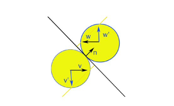
Consider a collision of two identical hard spheres in the center of momentum frame, so that $z=0$. Let $n$ be the unit vector pointing from the center of one particle to the center of the other at the moment of collision. (It does not matter from which to which; our expressions will be quadratic in $n$.) The result of the collision is exactly as if each particle undergoes specular reflection upon striking the plane through the point of contact that has unit normal $n$. As a result, the velocities of both particles are reflected about this plane, as shown in Figure 1.

Figure 1: Profile of the plane of reflection, with some normal lines indicated, along which the pre and post collisional velocities line up.

Clearly, the relative velocity $u=v-w$ of the two particles is also reflected about this plane, so that we have $u^{\prime}=u-2(u\cdot n)n$. This remains true if we translate out of the center of momentum frame. Also, since reflection is an isometry, $k^{\prime}=k-2(k\cdot n)n$. We therefore let $n$ stand in the role of $\omega$, and we have

$$k^{\prime}=k-2(k\cdot n)n\qquad{\rm and}\qquad n^{\prime}=n\ .$$ (A.4)

From this and (A.3) we obtain the full collision map:

$$\begin{cases}v^{\prime}&=\ v-((v-w)\cdot n)n\\[2.84526pt] w^{\prime}&=\ w+((v-w)\cdot n)n\\[2.84526pt] n^{\prime}&=\ n\end{cases}$$ (A.5)

Let us use $C_{r}$ to denote the collision map $C_{r}(v,w,n)=(v^{\prime},w^{\prime},n^{\prime})$ based on (A.5). Of course, $n$ and $-n$ lead to the same reflection, so that if we hold $v$ and $w$ fixed and vary $n$, we get a double cover of the set of possible post collisional velocities $(v^{\prime},w^{\prime})$ resulting from $(v,w)$. However, as is clear from the third line, as a transformation from $\Xi$ onto itself, $C_{r}$ is a bijection.

The next thing to observe is that $C_{r}$ is a measure preserving transformation on $\Xi$. Indeed, since the measure ${\rm d}v{\rm d}w{\rm d}n$ on $\Xi$ is also the measure ${\rm d}z{\rm d}u{\rm d}n$, going to polar coordinates in $u$, we have ${\rm d}v\ {\rm d}w\ {\rm d}n={\rm d}z\ {\rm d}|u|\ {\rm d}k\ {\rm d}n$. Here ${\rm d}n$ and ${\rm d}k$ are both the uniform measures on $S^{2}$ with total mass $4\pi$, which is consistent with our use of polar coordinates. Since it is clear from Fubini’s Theorem that ${\rm d}k{\rm d}n={\rm d}k^{\prime}{\rm d}n^{\prime}$, we have that ${\rm d}v^{\prime}{\rm d}w^{\prime}{\rm d}n^{\prime}={\rm d}v{\rm d}w{\rm d}n$. This gives us the collision kernel in the reflection representation

$$\langle Q(f,f),\varphi\rangle=\frac{1}{4\pi}\int_{{\mathord{\mathbb{R}}}^{3}}\int_{{\mathord{\mathbb{R}}}^{3}}\int_{S^{2}}f(v)f(w)[\varphi(v^{\prime})-\varphi(v)]\widetilde{\Phi}(|u|)\widetilde{B}(k\cdot n){\rm d}n{\rm d}v{\rm d}w\ .$$ (A.6)

Here, $\widetilde{\Phi}$ and $\widetilde{B}$ takes into account the difference rates of collisions and its dependence with respect to the strength of the relative velocity and the collision angle respectively and $\varphi$ is any test function.

Finally, since reflections are their own inverses, one sees that $C_{r}$ is its own inverse. Therefore, we may regard $(v^{\prime},w^{\prime})$ as pre collisional velocities that may result in the pair $(v,w)$ of post collisional velocities. Thus, in the “gain term” part of the integral for $Q(f,f)$, one can change variables

$$\int_{{\mathord{\mathbb{R}}}^{3}}\!\!\int_{{\mathord{\mathbb{R}}}^{3}}\!\!\int_{S^{2}}f(v)f(w)\varphi(v^{\prime})\widetilde{B}(k\cdot n){\rm d}n{\rm d}v{\rm d}w=\int_{{\mathord{\mathbb{R}}}^{3}}\!\!\int_{{\mathord{\mathbb{R}}}^{3}}\!\!\int_{S^{2}}f(v^{\prime})f(w^{\prime})\varphi(v)\widetilde{\Phi}(|u^{\prime}|)\widetilde{B}(k^{\prime}\cdot n^{\prime}){\rm d}n^{\prime}{\rm d}v^{\prime}{\rm d}w^{\prime}\ .$$

Now, recall that $\widetilde{B}$ is even, and note that $k^{\prime}\cdot n^{\prime}=-k\cdot n$ and $|u^{\prime}|=|u|$. Using this and the measure preserving property, we obtain

$$\int_{{\mathord{\mathbb{R}}}^{3}}\!\!\int_{{\mathord{\mathbb{R}}}^{3}}\!\!\int_{S^{2}}f(v^{\prime})f(w^{\prime})\varphi(v)\widetilde{\Phi}(|u^{\prime}|)\widetilde{B}(k^{\prime}\cdot n^{\prime}){\rm d}n^{\prime}{\rm d}v^{\prime}{\rm d}w^{\prime}=\int_{{\mathord{\mathbb{R}}}^{3}}\!\!\int_{{\mathord{\mathbb{R}}}^{3}}\!\!\int_{S^{2}}f(v^{\prime})f(w^{\prime})\varphi(v)\widetilde{\Phi}(|u|)\widetilde{B}(k\cdot n){\rm d}n{\rm d}v{\rm d}w\ .$$

Thus, we have

$$\langle Q(f,f),\varphi\rangle=\frac{1}{4\pi}\int_{{\mathord{\mathbb{R}}}^{3}}\int_{{\mathord{\mathbb{R}}}^{3}}\int_{S^{2}}[f(v^{\prime})f(w^{\prime})-f(v)f(w)]\varphi(v)\widetilde{\Phi}(|u|)\widetilde{B}(k\cdot n){\rm d}n{\rm d}v{\rm d}w\ ,$$

which allows us to write the collision kernel in the strong form:

$$Q(f,f)(v)=\frac{1}{4\pi}\int_{{\mathord{\mathbb{R}}}^{3}}\int_{S^{2}}[f(v^{\prime})f(w^{\prime})-f(v)f(w)]\widetilde{\Phi}(|u|)\widetilde{B}(k\cdot n){\rm d}n{\rm d}w\ .$$ (A.7)

Note that to specify everything needed to compute $Q(f,f)$, one needs only the first two lines of (A.5), and this is all that is usually written down in discussions of elastic collisions. However, in the inelastic case, the collisions are not reversible, since they dissipate energy, and so there is not such a simple relation between the pre and post collisional velocities. Thus, more care is required in the passage from the weak form of the collision kernel to the strong form, and it will be helpful to keep all three lines in (A.5), and remember that $C_{s}$ is a measure preserving bijection of $\Xi$ onto itself. Indeed, note that for fixed $n$, the map $(v,w)\mapsto(v^{\prime},w^{\prime})$ is a two to one, so dropping the third line, we would not have a bijection.

A.1.2 Swapping map:

As we have mentioned, there is another collision map which leads to a different way of writing down the collision kernel. This other way is less directly connected with the physics of hard sphere collisions, but it does have considerable mathematical advantages due to its simplicity, which is based on a simple swapping of $\omega$ and $k$. In this context, it is traditional to write $\sigma$ in place of $\omega$, and the very simple rule for computing $k^{\prime}$ and $\sigma^{\prime}$ in terms of $v$, $w$ and $\sigma$ is simply

$$k^{\prime}=\sigma\qquad{\rm and}\qquad\sigma^{\prime}=k\ .$$ (A.8)

As with (A.4), we use this and (A.3) to obtain the corresponding collision map:

$$\begin{cases}v^{\prime}&={\displaystyle\frac{v+w}{2}+\frac{|v-w|}{2}\sigma}\\[5.69054pt] w^{\prime}&={\displaystyle\frac{v+w}{2}-\frac{|v-w|}{2}\sigma}\\[5.69054pt] \sigma^{\prime}&=k={\displaystyle\frac{v-w}{|v-w|}}\end{cases}$$ (A.9)

Let us use $C_{s}$ to denote the swapping map $C_{s}(v,w,\sigma)=(v^{\prime},w^{\prime},\sigma^{\prime})$. Like $C_{r}$, $C_{s}$ is a measure preserving transformation on $\Xi$. As before, we note that the measure ${\rm d}v{\rm d}w{\rm d}\sigma$ on $\Xi$ is also the measure ${\rm d}z{\rm d}u{\rm d}\sigma$, and going to polar coordinates in $u$, we have ${\rm d}v\ {\rm d}w\ {\rm d}\sigma={\rm d}z\ {\rm d}|u|\ {\rm d}k\ {\rm d}\sigma$. In this form it is clear that the collision map for swapping is a measure preserving map, ${\rm d}v^{\prime}{\rm d}w^{\prime}{\rm d}\sigma^{\prime}\ =\ {\rm d}v{\rm d}w{\rm d}\sigma$. This gives us the collision kernel in the swapping representation:

$$\langle Q(f,f),\varphi\rangle=\frac{1}{4\pi}\int_{{\mathord{\mathbb{R}}}^{3}}\int_{{\mathord{\mathbb{R}}}^{3}}\int_{S^{2}}f(v)f(w)[\varphi(v^{\prime})-\varphi(v)]\Phi(|u|)B(k\cdot\sigma){\rm d}\sigma{\rm d}v{\rm d}w$$ (A.10)

where $\varphi$ is any test function, and as above $k$ denotes the unit vector in the direction of $v-w$, and $\Phi$ and $B$ gives the relative rates of the various kinematically possible collisions with respect to the strength of the relative velocity and the collision angle, and ${\rm d}\sigma$ is the uniform measure on $S^{2}$ with total mass $4\pi$.

Note that like $C_{r}$, $C_{s}$ is its own inverse, simply because the map in (A.8) is its own inverse. Thus, we may once more regard $(v^{\prime},w^{\prime})$ as a pair of pre collisional velocities. Changing variables, and using $k^{\prime}\cdot\sigma^{\prime}=k\cdot\sigma$, and the measure preserving property, we obtain the strong form

$$Q(f,f)(v)=\frac{1}{4\pi}\int_{{\mathord{\mathbb{R}}}^{3}}\int_{S^{2}}[f(v^{\prime})f(w^{\prime})-f(v)f(w)]B(k\cdot\sigma){\rm d}\sigma{\rm d}w\ .$$ (A.11)

Note that only the first two lines of (A.9) are required to compute $Q(f,f)$, and this is all that is usually written down in discussions of elastic collisions. However, it is worth noting explicitly that if one holds $\sigma$ fixed, and then just considers the transformation $(v,w)\mapsto(v^{\prime},w^{\prime})$ described by the first two lines, this transformation is not onto and not injective: While the direction of $u$ is arbitrary, the direction of $u^{\prime}$ is always that of $\sigma$. In the inelastic case, everything will be clear if we always keep in mind that the collision map is a bijection from $\Xi$ onto itself, and keep all three lines needed to specify this map.

There is one more important point to notice: The integral in (A.10) is unchanged if we swap $v$ and $w$; i.e., make the change of variables $(v,w,\sigma)\mapsto(w,v,\sigma)$. This transformation does not affect $v^{\prime}$ but it reverses the sign on $k$, and so we may replace $B(k\cdot\sigma)$ in (A.10) with $B(-k\cdot\sigma)$ without affecting $\langle Q^{+}(f,f),\varphi\rangle$. That is, only the symmetric part of $B$ contributes to the collision kernel, and we may freely require, by symmetrizing if need be, that $B$ is a symmetric function on $[-1,1]$. We shall always impose this symmetry requirement on our rate functions $B$.

A.1.3 Relations between representations

Our final business in this section is to relate these two representation of the gain term, and to determine in particular the relation between $\Phi$, $B$ and $\tilde{\Phi}$, $\tilde{B}$ in (A.10) and (A.6). The crucial fact is that both maps $(v,w,n)\mapsto(v^{\prime},w^{\prime},n^{\prime})$ and $(v,w,\sigma)\mapsto(v^{\prime},w^{\prime},\sigma^{\prime})$ yield the same pair $(v^{\prime},w^{\prime})$ if $\sigma$ and $n$ are related through $\sigma=k-2(k\cdot n)n$; i.e., if $\sigma$ is the reflection of $k$ about the plane normal to $n$. Indeed, since, for example,

$$\frac{v+w}{2}+\frac{v-w}{2}-((v-w)\cdot n)n\ =\ v-((v-w)\cdot n)n\ ,$$ (A.12)

the first lines of (A.9) and (A.5) coincide if we relate $n$ and $\sigma$ through

$$\frac{u}{2}-(u\cdot n)n=\frac{|u|}{2}\sigma\qquad{\rm or,\ equivalently}\qquad k-2(k\cdot n)n=\sigma\ .$$ (A.13)

Since $\sigma$ is the reflection of $k$ about the plane orthogonal to $n$, we recover $n$ (up to a sign) in terms of $\sigma$ and $k$ through:

$$n=\frac{u-|u|\sigma}{|u-|u|\sigma|}\qquad{\rm or,\ equivalently}\qquad n=\frac{k-\sigma}{|k-\sigma|}\ .$$ (A.14)

The fact that we only recover $n$ up to a sign does not matter; it is not $n$ itself, but only the plane normal to $n$ that matters in all computations we shall make. Finally, from (A.13) doing the $k\cdot$ operation over the formula for $k$, we have

$$|k\cdot n|=\sqrt{\frac{1-k\cdot\sigma}{2}}\ .$$ (A.15)

These formulas will be very useful in relating the $n$ representation and the $\sigma$ representation for inelastic collisions.

To work out the relation between $\Phi$, $B$ and $\tilde{\Phi}$, $\widetilde{B}$, we need just one more identity [3, 4]: For any test functions $\varphi$ on ${\mathord{\mathbb{R}}}^{3}$,

$$\int_{S^{2}}\varphi\left(\frac{u-|u|\sigma}{2}\right){\rm d}\sigma=\int_{S^{2}}\frac{2|u\cdot n|}{|u|}\varphi\left((u\cdot n)n\right){\rm d}n\ .$$ (A.16)

To see this, observe that if we define $\theta=\cos^{-1}(k\cdot\sigma)$ and $\chi=\cos^{-1}(k\cdot n)$, then from the reflection relation between $k$, $n$ and $\sigma$ in (A.13), we see that for $0\leq\chi\leq\pi/2$, $\theta=\pi-2\chi$, so that

$$\sin(\theta){\rm d}\theta=2\sin(2\chi){\rm d}\chi=4\cos(\chi)\sin(\chi){\rm d}\chi=4|k\cdot n|\sin(\chi){\rm d}\chi\ .$$

Thus, using (A.15),

$${\rm d}\sigma=4|k\cdot n|{\rm d}n\qquad{\rm and}\qquad{\rm d}n=\frac{1}{4}\sqrt{\frac{2}{1-k\cdot\sigma}}{\rm d}\sigma\ .$$ (A.17)

Finally, by taking into account that with $k$ fixed, $n\mapsto\sigma$ is a two to one cover of $S^{2}$, and since $(u-|u|\sigma)/2=(u\cdot n)n$ as noted in (A.13), we obtain the identity (A.16).

Now since $v^{\prime}$ can be expressed either in terms of $(u-|u|)\sigma/2$ or $(u\cdot n)n$, by equating the right hand sides of (A.10) and (A.6) which requires $\Phi=\tilde{\Phi}$ and $B(k\cdot\sigma){\rm d}\sigma=2\widetilde{B}(k\cdot n){\rm d}n$ since $n\mapsto\sigma$ is a two to one cover of $S^{2}$ and $\tilde{B}$ is symmetric, we obtain from (A.17) that

$$B(k\cdot\sigma)=\frac{\widetilde{B}\left(k\cdot n\right)}{\phantom{.}2|k\cdot n|}\ .$$ (A.18)

Then since from (A.13) we have $k\cdot\sigma=1-2(k\cdot n)^{2}$, we obtain

$$B(s)=\frac{\widetilde{B}\left(\sqrt{(1-s)/2}\right)}{2\sqrt{(1-s)/2}}\qquad{\rm and}\qquad\widetilde{B}(t)=2|t|B(1-2t^{2})\ ,$$ (A.19)

where $-1\leq s\leq 1$ and $-1\leq t\leq 1$.

A.2 The kinematics of inelastic collisions

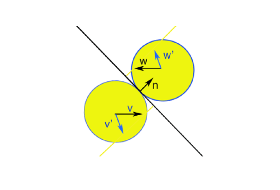
The kinematics of inelastic collisions is easiest to describe starting from the $n$ representation. As in the elastic case, viewed in the center of momentum frame, the collision behaves like a collision with a wall running normal to the direction vector $n$ pointing from the center of one ball to the center of the other ball at the point of contact. However, in the case of an inelastic collision with a wall, the component of the reflected velocity normal to the wall is reduced, while the component parallel to the wall is unchanged. Thus the rule for updating the relative velocity after the collision is this: Let $P_{n}$ denote the orthogonal projection onto the span of $n$. Then

$$P_{n}(v^{\prime}-w^{\prime})=-eP_{n}(v-w)\qquad\mbox{and}\qquad P_{n}^{\perp}(v^{\prime}-w^{\prime})=P_{n}^{\perp}(v-w)\ .$$

Thus, our rule for updating the relative velocity after the collision is a sort of reduced reflection

$$v^{\prime}-w^{\prime}=(v-w)-(1+e)((v-w)\cdot n)n\ ,$$

where the restitution coefficient $e$ satisfies $0\leq e\leq 1$. If $e=1$, then this is a reflection about the plane normal to $n$. If $e=0$, this simply cancels out the component of $v-w$ along $n$, which corresponds to a perfectly inelastic collision.

Figure 2: Profile of the plane of reflection, with some normal lines indicated, along which the pre and post collisional velocities line up in the inelastic case.

This gives us the inelastic reflection map with restitution coefficient $e$, denoted $C_{r,e}$: $C_{r,e}(v,w,n)=(v^{\prime},w^{\prime},n^{\prime})$ where

$$\begin{cases}v^{\prime}&=\ v-{\displaystyle\frac{1+e}{2}((v-w)\cdot n)n}\\[2.84526pt] w^{\prime}&=\ w+{\displaystyle\frac{1+e}{2}((v-w)\cdot n)n}\\[2.84526pt] n^{\prime}&=\ n\end{cases}$$ (A.20)

Note that with $u^{\prime}=v^{\prime}-w^{\prime}$, we have

$$|u^{\prime}|^{2}=|u|^{2}+(e^{2}-1)(u\cdot n)^{2}.$$ (A.21)

and

$$k^{\prime}=\frac{k-(1+e)(k\cdot n)n}{\sqrt{1+(e^{2}-1)(k\cdot n)^{2}}}\ .$$ (A.22)

We now have what we need to write down the gain term in the collision kernel in weak form using the inelastic reflection map:

$$\langle Q_{e}^{+}(f,f),\varphi\rangle=\frac{1}{4\pi}\int_{{\mathord{\mathbb{R}}}^{3}}\int_{{\mathord{\mathbb{R}}}^{3}}\int_{S^{2}}f(v)f(w)\varphi(v^{\prime})\widetilde{\Phi}(|u|)\widetilde{B}(k\cdot n){\rm d}n{\rm d}v{\rm d}w$$ (A.23)

where $\varphi$ and $k$ are as before, and again, $\widetilde{\Phi}$ and $\widetilde{B}$ gives the relative rates of the various kinematically possible collisions, and ${\rm d}n$ is the uniform measure on $S^{2}$ with total mass $4\pi$.

All formulas involving the Fourier transform, of which we shall make extensive use, are simplest in the $\sigma$–parameterization, and so we must translate the above inelastic parameterization into terms of $\sigma$. This is easy to do using (A.13) and (A.14). For example, the first line of (A.20) can be written as

$$v^{\prime}=\frac{v+w}{2}+\frac{u}{2}-\frac{1+e}{2}(u\cdot n)n=\frac{v+w}{2}+\frac{1-e}{4}u+\frac{1+e}{4}|u|\sigma\ ,$$

where (A.13) was used to eliminate $n$ in favor of $\sigma$. In the same way, we translate the second line, and find $w^{\prime}=\frac{v+w}{2}-\frac{1-e}{4}u-\frac{1+e}{4}|u|\sigma$, and it follows that $u^{\prime}=\frac{1-e}{2}u+\frac{1+e}{2}|u|\sigma$, so that

$$|u^{\prime}|^{2}=|u|^{2}\left(\frac{1+e^{2}}{2}+\frac{1-e^{2}}{2}k\cdot\sigma\right)\ ,$$ (A.24)

and

$$k^{\prime}=\frac{(1-e)k+(1+e)\sigma}{\sqrt{2(1+e^{2})+2(1-e^{2})k\cdot\sigma}}\ .$$ (A.25)

Finally, from (A.20) we have $(n\cdot u^{\prime})n=-e(n\cdot u)n$. Then from (A.13) we have

$$u^{\prime}-|u^{\prime}|\sigma^{\prime}=2(u^{\prime}\cdot n)n=-2e(u\cdot n)n=-e(u-|u|\sigma)\ .$$

solving for $\sigma^{\prime}$ we find

$$\sigma^{\prime}=k^{\prime}+e\frac{|u|}{|u^{\prime}|}(k-\sigma)\ .$$

Using the expressions just derived for $|u^{\prime}|$ and $k^{\prime}$, we find

$$\sigma^{\prime}=\frac{(1+e)k+(1-e)\sigma}{\sqrt{2(1+e^{2})+2(1-e^{2})k\cdot\sigma}}\ .$$ (A.26)

This gives us the inelastic swapping map with restitution coefficient $e$, denoted $C_{s,e}$: $C_{s,e}(v,w,\sigma)=(v^{\prime},w^{\prime},\sigma^{\prime})$ where

$$\begin{cases}v^{\prime}&={\displaystyle\frac{v+w}{2}+\frac{1-e}{4}(v-w)-\frac{1+e}{4}|v-w|\sigma}\\[8.53581pt] w^{\prime}&={\displaystyle\frac{v+w}{2}-\frac{1-e}{4}(v-w)+\frac{1+e}{4}|v-w|\sigma}\\[8.53581pt] \sigma^{\prime}&={\displaystyle\frac{(1+e)k+(1-e)\sigma}{\sqrt{2(1+e^{2})+2(1-e^{2})k\cdot\sigma}}}\end{cases}$$ (A.27)

We now have what we need to write down the gain term in the collision kernel in weak form for inelastic collision in the $\sigma$ representation: The basic expression that defines the gain term is

$$\langle Q_{e}^{+},\varphi\rangle=\frac{1}{4\pi}\int_{{\mathord{\mathbb{R}}}^{3}}\int_{{\mathord{\mathbb{R}}}^{3}}\int_{S^{2}}f(v)f(w)\varphi(v^{\prime})\Phi(|u|)B(k\cdot\sigma){\rm d}\sigma{\rm d}v{\rm d}w$$ (A.28)

where $\varphi$ is any test function, and as above $k$ denotes the unit vector in the direction of $v-w$, and $\Phi$ and $B$ gives the relative rates of the various kinematically possible collisions, and ${\rm d}\sigma$ is the uniform measure on $S^{2}$ with total mass $4\pi$. Let us remark that being the $n$-representation more physically meaningful, the $\sigma$-representation is a nice mathematical device to derive estimates in both the weak and the strong formulation.

A.3 Strong form of the inelastic collision kernel

Finally, we want to derive the strong form of the gain term, and for this we need the precollisional velocities $v^{*}$ and $w^{*}$. That is, given a collision map $C$, we define $(v^{*},w^{*},\omega^{*})=C^{-1}(v,w,\omega)$. It is very easy to invert the the transformation $(v,w,n)\mapsto(v^{\prime},w^{\prime},n^{\prime})$ in the reflection parameterization (A.20): Simply use a restitution coefficient of $1/e$. This gives us $C_{r,e}^{-1}(v,w,n)=(v^{*},w^{*},n^{*})$ where

$$\begin{cases}v^{*}&=\ v-{\displaystyle\frac{1+e}{2e}((v-w)\cdot n)n}\\[5.69054pt] w^{*}&=\ w+{\displaystyle\frac{1+e}{2e}((v-w)\cdot n)n}\\[5.69054pt] n^{*}&=\ n\end{cases}$$ (A.29)

Note that with $u^{*}=v^{*}-w^{*}$, we have

$$|u^{*}|^{2}=|u|^{2}+\left(\frac{1}{e^{2}}-1\right)(u\cdot n)^{2}=|u|^{2}\left(1+\left(\frac{1}{e^{2}}-1\right)(k\cdot n)^{2}\right)\$$ (A.30)

and $u^{*}\cdot n=-\frac{1}{e}u\cdot n$. Combining these we have

$$k^{*}\cdot n=-\frac{k\cdot n}{\sqrt{e^{2}+(1-e^{2})(k\cdot n)^{2}}}\ .$$ (A.31)

Now, the determinant of the Jacobian matrix for the transformation in (A.20) is easily seen to be

$$\left(\frac{1-e}{2}\right)^{2}-\left(\frac{1+e}{2}\right)^{2}=-e\ ,$$

independent of $n$, so that the Jacobian itself is $e$. Thus, the determinant of the Jacobian matrix of the inverse transformation is $-1/e$, also independent of $n$, so the Jacobian itself is $1/e$. We thus can rewrite (A.23) as

$$\langle Q_{e}^{+},\varphi\rangle=\frac{1}{4\pi}\int_{{\mathord{\mathbb{R}}}^{3}}\int_{{\mathord{\mathbb{R}}}^{3}}\int_{S^{2}}f(v^{*})f(w^{*})\varphi(v)\widetilde{\Phi}(|u^{*}|)\frac{\widetilde{B}(k^{*}\cdot n)}{e}{\rm d}n{\rm d}v{\rm d}w$$ (A.32)

where $\varphi$ and $\widetilde{B}$ are as before, and $k^{*}=v^{*}-w^{*}$. Taking into account (A.30) and (A.31) and the fact that $\widetilde{B}$ is even,

$$Q_{e}^{+}(f,f)(v)=\frac{1}{4\pi}\int_{{\mathord{\mathbb{R}}}^{3}}\int_{S^{2}}f(v^{*})f(w^{*})\widetilde{\Phi}_{e}^{+}(|u|,k\cdot n)\widetilde{B}_{e}^{+}\left(k\cdot n\right){\rm d}n{\rm d}w\ ,$$ (A.33)

where $\widetilde{B}_{e}^{+}$

$$\widetilde{B}_{e}^{+}(s)=\widetilde{B}\left(\frac{s}{\sqrt{e^{2}+(1-e^{2})s^{2}}}\right)\frac{1}{e}\ ,$$ (A.34)

and

$$\widetilde{\Phi}_{e}^{+}(r,s)=\widetilde{\Phi}\left(\frac{r}{e}\sqrt{e^{2}+(1-e^{2})s^{2}}\right)\ .$$ (A.35)

Then, using the identities in (A.13) once more, we may translate (A.29) into the $\sigma$ parameterization, and obtain $C_{s,e}^{-1}(v,w,\sigma)=(v^{*},w^{*},\sigma^{*})$ where

$$\begin{cases}v^{*}&=\ {\displaystyle\frac{v+w}{2}-\frac{1-e}{4e}(v-w)+\frac{1+e}{4e}|v-w|\sigma}\\[8.53581pt] w^{*}&=\ {\displaystyle\frac{v+w}{2}+\frac{1-e}{4e}(v-w)-\frac{1+e}{4e}|v-w|\sigma}\\[8.53581pt] \sigma^{*}&={\displaystyle\frac{(1+e)k-(1-e)\sigma}{\sqrt{2(1+e^{2})-2(1-e^{2})k\cdot\sigma}}}\end{cases}$$ (A.36)

Along the way, we find, using (A.13) and (A.14) as before,

$$|u^{*}|^{2}=\frac{|u|^{2}}{2e^{2}}\left((1+e^{2})-(1-e^{2})(k\cdot\sigma)\right)\ .$$ (A.37)

and

$$k^{*}=\frac{(1+e)\sigma-(1-e)k}{\sqrt{2(1+e^{2})-2(1-e^{2})k\cdot\sigma}}\ .$$ (A.38)

Combining these we have

$$|k^{*}\cdot n|=\sqrt{\frac{1-k\cdot\sigma}{(1+e^{2})-(1-e^{2})k\cdot\sigma}}\ .$$ (A.39)

Now, we use (A.17) and (A.37) to translate $\widetilde{B}(k^{*}\cdot n){\rm d}n$ into terms of $\sigma$. We find, remembering that $\widetilde{B}$ is even:

$$\widetilde{B}(k^{*}\cdot n){\rm d}n=\frac{1}{4}\widetilde{B}\left(\sqrt{\frac{1-k\cdot\sigma}{(1+e^{2})-(1-e^{2})k\cdot\sigma}}\right)\sqrt{\frac{2}{1-k\cdot\sigma}}{\rm d}\sigma\ .$$

Next, we use (A.19) to express this in terms of $B$ in place of $\widetilde{B}$: We obtain:

$$\widetilde{B}(k^{*}\cdot n){\rm d}n=B\left(\frac{(1+e^{2})k\cdot\sigma-(1-e^{2})}{(1+e^{2})-(1-e^{2})k\cdot\sigma}\right)\frac{\sqrt{2}}{\sqrt{{(1+e^{2})-(1-e^{2})k\cdot\sigma}}}{\rm d}\sigma\ .$$

Moreover, using (A.31), we have

$$\widetilde{\Phi}(|u^{*}|)=\Phi(|u^{*}|)=\Phi\left(\frac{|u|}{\sqrt{2}e}\sqrt{(1+e^{2})-(1-e^{2})(k\cdot\sigma)}\right)\ .$$

Therefore, defining the function $B_{e}^{+}$ by

$$B_{e}^{+}(s)=B\left(\frac{(1+e^{2})s-(1-e^{2})}{(1+e^{2})-(1-e^{2})s}\right)\frac{\sqrt{2}}{\sqrt{{(1+e^{2})-(1-e^{2})s}}}\frac{1}{e}$$

and the function

$$\Phi_{e}^{+}(r,s)=\Phi\left(\frac{r}{\sqrt{2}e}\sqrt{(1+e^{2})-(1-e^{2})s}\right)\ ,$$

we have

$$Q_{e}^{+}(f,f)(v)=\frac{1}{4\pi}\int_{{\mathord{\mathbb{R}}}^{3}}\int_{S^{2}}f(v^{*})f(w^{*})\Phi_{e}^{+}(|u|,k\cdot\sigma)B_{e}^{+}(k\cdot\sigma){\rm d}\sigma{\rm d}w\ .$$ (A.40)

The change of variable formulas that we have deduced in this section, suffice not only to allow us to write down the strong form of the collision kernel, but also to prove the following somewhat more general result:

A.1 THEOREM.

Let $K$ be any continuous real valued function on $\Xi\times\Xi$. Then

$$\frac{1}{4\pi}\int_{{\mathord{\mathbb{R}}}^{3}}\int_{{\mathord{\mathbb{R}}}^{3}}\int_{S^{2}}K[C_{s,e}^{-1}(v,w,\sigma),(v,w,\sigma)]\Phi_{e}^{+}(|u|,k\cdot\sigma)B_{e}^{+}(k\cdot\sigma){\rm d}\sigma{\rm d}w{\rm d}v\\ =\frac{1}{4\pi}\int_{{\mathord{\mathbb{R}}}^{3}}\int_{{\mathord{\mathbb{R}}}^{3}}\int_{S^{2}}K[(v,w,\sigma),C_{s,e}(v,w,\sigma)]\Phi(|u|)B(k\cdot\sigma){\rm d}\sigma{\rm d}w{\rm d}v$$ (A.41)

and

$$\frac{1}{4\pi}\int_{{\mathord{\mathbb{R}}}^{3}}\int_{{\mathord{\mathbb{R}}}^{3}}\int_{S^{2}}K[C_{r,e}^{-1}(v,w,n),(v,w,n)]\widetilde{\Phi}_{e}^{+}(|u|,k\cdot n)\widetilde{B}_{e}^{+}(k\cdot n){\rm d}n{\rm d}w{\rm d}v\\ =\frac{1}{4\pi}\int_{{\mathord{\mathbb{R}}}^{3}}\int_{{\mathord{\mathbb{R}}}^{3}}\int_{S^{2}}K[(v,w,n),C_{r,e}(v,w,n)]\widetilde{\Phi}(|u|)\widetilde{B}(k\cdot n){\rm d}n{\rm d}w{\rm d}v\ ,$$ (A.42)

where $\Phi=\widetilde{\Phi}$ and $B$ and $\widetilde{B}$ are related by (A.19).

References

- [1] M. Bisi, J.A. Carrillo, G. Toscani, Contractive Metrics for a Boltzmann equation for granular gases: Diffusive equilibria, J. Statist. Phys. 118 (2005), 301–331.
- [2] M. Bisi, J.A. Carrillo, G. Toscani, Decay rates in probability metrics towards homogeneous cooling states for the inelastic Maxwell model, J. Statist. Phys. 124 (2006), 625–653.
- [3] A.V. Bobylev, Fourier transform method in the theory of the Boltzmann equation for Maxwellian molecules, Dokl. Akad. Nauk USSR 225 (1975), 1041-1044.
- [4] A.V. Bobylev, The theory of the nonlinear spatially uniform Boltzmann equation for Maxwell molecules, Sov. Sci. Rev. C. Math. Phys. 7 (1988), 111–233.
- [5] A.V. Bobylev, J.A. Carrillo, I. Gamba, On some properties of kinetic and hydrodynamic equations for inelastic interactions, J. Statist. Phys. 98 (2000), 743–773; Erratum on: J. Statist. Phys. 103, (2001), 1137–1138.
- [6] A.V. Bobylev, C. Cercignani, Self-similar asymptotics for the Boltzmann equation with inelastic and elastic interactions, J. Statist. Phys. 110 (2003), 333-375.
- [7] A.V. Bobylev, C. Cercignani, I. Gamba, Generalized Maxwell models and self-similar asymptotics, Lecture Notes in Mathematics, Springer, G. Capriz, P. Giovine and P. M. Mariano Edts, in press (2006).
- [8] A.V. Bobylev, C. Cercignani, I. Gamba, On the self-similar asymptotics for generalized non-linear kinetic Maxwell models, to appear in Comm. Math. Phys.
- [9] A.V. Bobylev, C. Cercignani, G. Toscani, Proof of an asymptotic property of self-similar solutions of the Boltzmann equation for granular materials, J. Statist. Phys. 111 (2003), 403-417.
- [10] F. Bolley, J.A. Carrillo, Tanaka Theorem for Inelastic Maxwell Models, Comm. Math. Phys. 276 (2007), 287–314.
- [11] E.A. Carlen, M.C. Carvalho, Strict entropy production bounds and stability of the rate of convergence to equilibrium for the Boltzmann equation, J. Statist. Phys. 67 (1992), 575–608.
- [12] E.A. Carlen, E. Gabetta, G. Toscani, Propagation of smoothness and the rate of exponential convergence to equilibrium for a spatially homogeneous Maxwellian gas, Commun. Math. Phys. 305 (1999), 521–546.
- [13] J. A. Carrillo, G. Toscani, Contractive probability metrics ans asymptotic behavior of dissipative kinetic equations, Riv. Mat. Univ. Parma 6 (2007), 75–198.
- [14] I. Csiszar, Information-type measures of difference of probability distributions and indirect observations, Stud. Sci. Math. Hung. 2 (1967), 299–318.
- [15] L. Desvillettes, About the Use of the Fourier Transform for the Boltzmann Equation, Rivista Matematica dell’Universit di Parma 7 (2003), 1–99.
- [16] M.H. Ernst, R. Brito, High energy tails for inelastic Maxwell models, Europhys. Lett. 58 (2002), 182-187.
- [17] M.H. Ernst, R. Brito, Scaling solutions of inelastic Boltzmann equation with over-populated high energy tails, J. Statist. Phys. 109 (2002), 407-432.
- [18] I. Gamba, V. Panferov, C. Villani, On the Boltzmann equation for diffusively excited granular media, Comm. Math. Phys. 246 (2004), 503–541.
- [19] L. Gross, Logarithmic Sobolev inequalities, Amer. J. of Math. 97 (1975), 1061–1083.
- [20] S. Kullback, R.A. Leibler, On Information and Sufficiency, Annals of Mathematical Statistics 22 (1951), 79-86.
- [21] P.L.Lions, G.Toscani, A strenghtened central limit theorem for smooth densities, J. Funct. Anal. 128 (1995), 148-167.
- [22] G. Toscani, Sur l’inégalité logarithmique de Sobolev, C.R. Acad. Sc. Paris A 324 série 1 (1997), 689-694.
- [23] C. Villani, Fisher information estimates for Boltzmann’s collision operator, J. Math. Pures Appl. 77 (1998), 821-837.
- [24] C. Villani, Mathematics of granular materials, J. Statist. Phys. 124 (2006), 781-822.
- [25] X. Zhang, Regularity and long time behavior of the Boltzmann equation for granular gases, J. Math. Anal. Appl. 324 (2006), 650-662.