The role of internal chain dynamics on the rupture kinetics
of adhesive contacts

Abstract

We study the forced rupture of adhesive contacts between monomers that are not covalently linked in a Rouse chain. When the applied force ($f$) to the chain end is less than the critical force for rupture ($f_{c}$), the reversible rupture process is coupled to the internal Rouse modes. If $f/f_{c}$$>$$1$ the rupture is irreversible. In both limits, the non-exponential distribution of contact lifetimes, which depends sensitively on the location of the contact, follows the double-exponential (Gumbel) distribution. When two contacts are well separated along the chain, the rate limiting step in the sequential rupture kinetics is the disruption of the contact that is in the chain interior. If the two contacts are close to each other, they cooperate to sustain the stress, which results in an “all-or-none” transition.

Nanomanipulation of biological molecules by force can be used to explore and control their energy landscapes at the single molecule level BlockAnnRevBiophys2007TinocoPNAS07FernandezPNAS07 . The challenge is to solve the inverse problem, namely, to extract the unbinding pathways and structural features pertaining to the systems of interest from measurements such as the force-extension curves, lifetime distribution of adhesive contacts, and unbinding force distributions. From these data, many characteristics of the energy landscape (roughness, barrier height, and movement of the transition states) have been obtained using theoretical models HyeonPNAS03DudkoPNAS03 ; BarsegovPRL05 . In these models, the force-induced unbinding transitions from the bound state (for example folded conformations of RNA) are presumed to occur irreverisbly along a one dimensional reaction coordinate, $R$, that is conjugate to the applied force, $f$. In this picture, $f$ “tilts” the energy landscape, thus rendering the bound state unstable when $f$ exceeds a critical value. On the other hand, detailed simulations of forced unfolding of proteins and RNA Hyeon06BiophysJ show that collective topology-dependent events that describe the internal dynamics BarsegovPRL05 are coupled to $R$. Thus, it is important to develop solvable models for force-induced disruption of “folded” structures starting from a well-defined Hamiltonian.

In this letter, we illustrate the interplay between internal polymer dynamics and the rupture kinetics of intramolecular adhesive contacts between monomers. Such a model is a caricature of forced-unfolding of RNA hairpins BlockAnnRevBiophys2007TinocoPNAS07FernandezPNAS07 where the adhesive contact mimics the stability of the stem. Using an exactly solvable Rouse model, with one or two adhesive contacts between monomers that are not covalently linked, we address the following questions: (i) For a single adhesive contact, how do the lifetime distribution functions vary with the backbone distance between monomers $r$ and $s$ that are in adhesive contact? (ii) To what extent is the binding of a ruptured contact influenced by $f$ and the internal polymer motions?

The model: Consider a Rouse chain with $N$ identical monomers, connected by a harmonic spring with the equilibrium distance $a$, with a single adhesive contact $(r,s)$ between two non-covalently linked monomers $r$ and $s$, $1$$\leq$$r$$<$$s$$\leq$$N$. The first monomer is fixed, and a constant force ${\bf f}$$=$$f$${\bf x}$ is applied to the $N^{th}$ monomer in the direction parallel to the end-to-end vector ${\bf X}$. Letting ${\bf R}_{m}$$=$$\{R_{m}^{x},R_{m}^{y},R_{m}^{z}\}$ be the monomer position, ($m$$=$$1,2,\ldots,N$), the equation of motion is, $\xi{{d}\over{dt}}{\bf R}_{m}$$=$$-\nabla_{{\bf R}_{m}}$$H(\{{\bf R}_{m}\})$$+$${\bf F}_{m}$ where $\nabla_{{\bf R}_{m}}$$\equiv$$\partial/\partial{\bf R}_{m}$, $\xi$ is the friction cefficient, and ${\bf F}_{m}$ is the random force with zero mean and $\langle F_{m}^{\alpha}(t)F_{n}^{\beta}(0)\rangle$$=$$2\xi k_{B}T\delta_{mn}\delta_{\alpha\beta}\delta(t)$ ($\alpha$, $\beta$$=$$x$, $y$, $z$). We model the adhesive contact $(r,s)$ using a harmonic potential with a spring constant, $\kappa$$=$$3k_{B}T/b^{2}$, where $b$ is the equilibrium contact distance. The Hamiltonian with a single contact under tension is taken to be $H$$=$$H_{0}$$+$${\bf f_{N}}({\bf R}_{N}-{\bf R}_{1})$ where

$$H_{0}={{3k_{B}T}\over{2a^{2}}}\sum_{n=2}^{N}({\bf R}_{n}-{\bf R}_{n-1})^{2}+{{3k_{B}T}\over{2b^{2}}}\Theta(B-|{\bf R}_{rs}|){\bf R}_{rs}^{2}$$ (1)

with ${\bf R}_{rs}$$=$${\bf R}_{r}$$-$${\bf R}_{s}$, and $\Theta(x)$ is the Heaviside step function. The contact is ruptured when $|{\bf R}_{rs}|$$\geq$$B$. The probability density function (pdf) of the $(r,s)$-contact lifetimes is obtained as $p_{rs}(t,f)$$=$$-dP_{rs}(t,f)/dt$, where $P_{rs}(t)$, the probability that the adhesive contact remains intact, is $P_{rs}(t,f)$$=$${{\int_{|{\bf R_{rs}}|\leq B}d^{3}{\bf R}_{rs}\int d^{3}{\bf R}_{rs}^{0}Q_{f}({\bf R}_{rs},t;{\bf R}_{rs}^{0})P_{I}({\bf R}_{rs}^{0})}\over{\int d^{3}{\bf R}_{rs}\int d^{3}{\bf R}_{rs}^{0}Q_{f}({\bf R}_{rs},t;{\bf R}_{rs}^{0})P_{I}({\bf R}_{rs}^{0})}}$. Here, $Q_{f}({\bf R}_{rs},t;{\bf R}_{rs}^{0})$, the conditional probability for the contact distance ${\bf R}_{rs}$ with the initial distribution $P_{I}({\bf R}_{rs}^{0})$ of the contact distance, ${\bf R}_{rs}^{0}$, is given in terms of ${\bf C_{1}}(t)$$=$$\langle{\bf R}_{rs}(t)\rangle$, and $C_{2}(t)$$=$$\langle[{\bf R}_{rs}(t)-\langle{\bf R}_{rs}(t)\rangle]^{2}\rangle$ by

$$Q_{f}({\bf R}_{rs},t;{\bf R}_{rs}^{0})=\left[{{3}\over{2\pi C_{2}(t)}}\right]^{{3}\over{2}}\exp{\left[-{{3({\bf R}_{rs}-{\bf C_{1}}(t))^{2}}\over{2C_{2}(t))}}\right]}$$ (2)

We define the $N$$\times$$3$-matrices for positions, ${\bf R}(t)$$\equiv$$({\bf R}_{1}(t),{\bf R}_{2}(t),\ldots,{\bf R}_{N}(t))^{\dagger}$, random forces, ${\bf F}(t)$ $\equiv$$({\bf F}_{1}(t),{\bf F}_{2}(t),\ldots,{\bf F}_{N}(t))^{\dagger}$, and the applied force, ${\bf f}$$\equiv$$({\bf 0},{\bf 0},\ldots,{\bf f}_{N})^{\dagger}$, where “$\dagger$” denotes the adjoint $3$$\times$$N$ matrix. The equation of motion in matrix form is ${{d}\over{dt}}{\bf R}+{\bf M}{\bf R}={{1}\over{\xi}}{\bf F}+{{1}\over{\xi}}{\bf f}$ with the $N$$\times$$N$ matrix ${\bf{M}}$$=$$\omega_{0}({\bf{A}}_{0}$$+$$\gamma{\bf{A}}_{1})$. The tridiagonal Rouse matrix is ${\bf{A}}_{0}$, with $a^{0}_{1,1}$$=$$a^{0}_{N,N}$$=$$1$, $a^{0}_{m,m}$$=$$2$, and $a^{0}_{m,m+1}$$=$$a^{0}_{m-1,m}$$=$$-1$ 20 , and $\omega_{0}$$=$$3k_{B}T/2a^{2}$. The interaction between monomers $r$ and $s$ are included in ${\bf{A}}_{1}$, with $a^{1}_{r,r}$$=$$a^{1}_{s,s}$$=$$1$ and $a^{1}_{r,s}$$=$$a^{1}_{r,s}$$=$$-1$. The strength of the adhesive contact, relative to the harmonic bond is $\gamma$$=$$(a/b)^{2}$.

Integration of the equation of motion gives ${\bf R}(t)$$=$${\bf G}(t)$${\bf R}(0)$$+$$(1/\xi)$$\int_{0}^{t}dt^{\prime}{\bf G}(t^{\prime})({\bf F}(t^{\prime})$$+$${\bf f})$, where ${\bf G}(t)$ is the Greens function; ${\bf G}(\omega)$$\equiv$$\left[i\omega{\bf I}+{\bf M}\right]^{-1}$ in the Fourier domain. To compute ${\bf C_{1}}(t)$ and $C_{2}(t)$, we must invert ${\bf G}(\omega)$. We rewrite ${\bf A}_{1}$$=$${\bf P}{\bf P}^{\dagger}$, where $\bf{P}$ is an $N$$\times$$1$ vector with non-zero elements $P_{r}$$=$$1$ and $P_{s}$$=$$-1$, and ${\bf G}(\omega)$$=$${\bf G}_{0}(\omega)$$-$${\bf G}_{0}(\omega){\bf P}$$[{{1}\over{\gamma w_{0}}}{\bf I}+{\bf P}^{\dagger}{\bf G}_{0}(\omega){\bf P}]^{-1}$${\bf P}^{\dagger}{\bf G}_{0}(\omega)$ 242522 , where the matrix elements $G_{0}(\omega)_{mn}$$=$$[i\omega{\bf I}$$+$${\bf M}_{0}]_{mn}^{-1}$$=$${{1}\over{N}}$$\sum_{p}{{\cos{[p\pi n/N]}\cos{[p\pi m/N]}}\over{i\omega+\lambda_{p}w_{0}}}$ and $\lambda_{p}$$=$$\pi^{2}p^{2}/N^{2}$ are the eigenmodes ($p$$=$$0,1,\ldots,N$) 20 .

The pdf of contact lifetimes for a single contact: Constraining the first residue of the chain is equivalent to excluding $\lambda_{0}$$=$$0$, which defines the overall translation of the chain. The results are presented by including the first ten modes for $N$$=$$100$, $a$$=$$0.4nm$, the diffusion coefficient, $D$$=$$10^{6}$$nm^{2}/s$, and $k_{B}T$$=$$4.1$$pN$$nm$. We chose $P_{I}({\bf R}_{rs}^{0})$$=$${{1}\over{4\pi(B/2)^{2}}}$$\delta(|{\bf R}_{rs}^{0}|-B/2)$, with the rupture distance set to $B$$=$$2a$. To assess the effect of the strength of the adhesive contact on the contact rupture kinetics, we used $\gamma$$=$$1$ (strong contact) and $\gamma$$=$$0.01$ (weak contact). The critical equilibrium force required to rupture the contact is $f_{c}$$=$$(3k_{B}TB/b^{2})$; $f_{c}$$=$$31pN$ for $\gamma$$=$$1$, and $f_{c}$$=$$0.31pN$ for $\gamma$$=$$0.01$. The values of $f$ were set to $f$$=$$1pN$ (weak force) and $f$$=$$40pN$ (strong force). At $f$$=$$1pN$, $f/f_{c}$$\ll$$1$ for $\gamma$$=$$1$, and $f/f_{c}$$\sim$$1$ for $\gamma$$=$$0.01$; at $f$$=$$40pN$, $f/f_{c}$$>$$1$ for $\gamma$$=$$1$ and $f/f_{c}$$\gg$$1$ for $\gamma$$=$$0.01$.

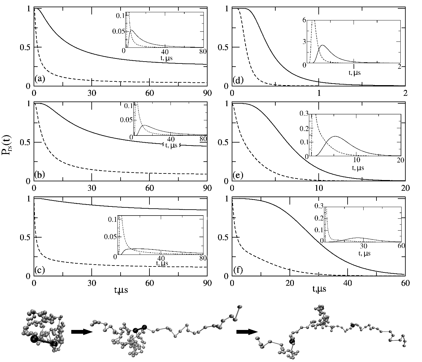
Figure 1: The survival probabilities $P_{rs}(t)$ for a single contact $(r,s)$$=$$(1,100)$ ($\mathbf{a}$, $\mathbf{d}$), $(20,80)$ ($\mathbf{b}$, $\mathbf{e}$), and $(40,60)$ ($\mathbf{c}$, $\mathbf{f}$), with ${f}$$=$$1$pN ($\mathbf{a}$$-$$\mathbf{c}$) and $40$pN ($\mathbf{d}$$-$$\mathbf{f}$), and with $\gamma$$=$$1$ (solid lines) and $0.01$ (dashed lines). The lifetime distributions $p_{rs}(t)$ are shown in the insets. Notice the variations in time scales in the panels. The chain structures for the intact single contact $(20,80)$, before and after the rupture are shown.

The survival probabilities $P_{rs}(t)$ (Fig. 1) of the adhesive contact at $f$$=$$1pN$ and $f$$=$$40pN$ for $\gamma$$=$$0.01$ and $\gamma$$=$$1$ show striking variations with respect to $|r-s|$. For a fixed $f$ (low forces with $f/f_{c}$$\ll$$1$ or $\sim$$1$) the decay of $P_{rs}(t)$ not only depends on the strength of the contact, but also on its location. At $f$$=$$1pN$, $P_{rs}(t)$ for strong and weak bonds display markedly different kinetics, with $P_{rs}(t)$ for weak contact $(r,s)$$=$$(1,100)$ and $(20,80)$ decaying to values close to zero on $30\mu s$ timescale (Figs. 1a and 1b). However, for $(r,s)$$=$$(40,60)$ the asymptotic value of $P_{rs}(t$$\to$$\infty)$$=$$P_{rs}^{eq}$$\approx$$0.12$ (Fig. 1c). Surprisingly, $P_{rs}(t)$s for $(r,s)$$=$$(20,80)$ and $(40,60)$ for strong bonds are qualitatively similar (Fig. 1b and 1c) and approach higher values of $P_{rs}^{eq}$$\approx$$0.42$ and $0.85$ respectively, whereas $P_{rs}^{eq}$$\approx$$0.26$ for $(r,s)$$=$$(1,100)$ (Fig. 1a). Thus, the rupture of contacts in the middle of the chain is strongly dependent on the coupling between the internal modes of the chain and the dynamics of instability due to the applied force. We refer to this as the “internal motion dominated” (IMD) regime. The stochastic nature of the bond rupture kinetics is also reflected in the decay of $P_{rs}(t)$ for strong and weak bonds. For $(r,s)$$=$$(1,100)$, $P_{rs}(t)$ decays faster to lower $P_{rs}^{eq}$, due to larger chain fluctuations at the chain ends compared to contacts $(r,s)$$=$$(20,80)$ and $(40,60)$ in the middle of the chain. In contrast to low forces, for $f/f_{c}$$>$$1$, $P_{rs}(t)$ for all contacts decay to zero at long times, regardless of the contact strength (Figs. 1d-1f). However, $P_{rs}(t)$ for strong contact $(r,s)$$=$$(40,60)$, which is close to the midpoint of the chain, decays to zero on a much slower $40\mu s$ timescale, compared to $10\mu s$ and $1\mu s$ timescale for $(r,s)$$=$$(20,80)$ and $(1,100)$. At $f$$=$$40pN$, $P_{rs}(t)$ for weak contacts decay to zero on similar time scales (Figs. 1d-1f) which shows that at large forces rupture kinetics is solely determined by the instability caused by the applied tension, with chain dynamics playing relatively minor role. Thus, as $f/f_{c}$ increases, the rupture kinetics become increasingly “tension dominated”, i.e. contact rupture is due to the applied force. Interestingly, there is a significant plateau in the decay of $P_{rs}(t)$ especially for $\gamma$$=$$1$. The duration of the plateau increases as $|r-s|$ decreases and $f$ increases (Figs. 1d-1f), and shows that the kinetics of rupture is non-exponential.

The lifetime distributions, $p_{rs}(t)$ (insets in Fig. 1), show longer tails for the stronger contacts; $p_{rs}(t)$ for the interior contact $(40,60)$ (Figs. 1c and 1f), does not have a pronounced dependence on $f$ compared to $p_{rs}(t)$ for contacts $(20,80)$ and $(1,100)$ (Figs. 1a, 1b, and 1d and 1e). In particular, $p_{rs}(t)$ at $f$$=$$1pN$ and $f$$=$$40pN$ agree quantitatively for strong and weak $(40,60)$-contacts. This implies that the disruption of the interior contacts is mediated by internal chain motions, and hence is in the IMD regime even at high $f$. The influence of internal motion of the chain on the contact rupture kinetics is also reflected in the width of $p_{rs}(t)$s which broadens for remote contacts $(20,80)$ and $(40,60)$.

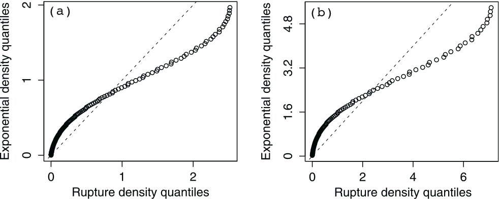
Figure 2: The $Q$$-$$Q$ plots (empty circles) of lifetimes $p_{rs}(t)$ for single contact $(r,s)$$=$$(1,100)$ ($x$-axis) versus lifetimes $p_{exp}(t)$ ($y$-axis), for $f$$=$$40$pN and $\gamma$$=$$1$ ($\mathbf{a}$) and $\gamma$$=$$0.01$ ($\mathbf{b}$). The rate $K$ in $p_{exp}(t)$ is set to the inverse of the average contact lifetime (the maximum likelihood estimate) 1919a .

Contact lifetime pdf is non-exponential: Forced rupture of noncovalent bonds is often described using two-state kinetics, $(rs)$$\to$$0$, which corresponds to the exponential pdf of contact lifetimes, $p_{exp}(t)$$=$$K$$\exp{[-Kt]}$ where $K$ is rupture rate. The results for $p_{rs}(t)$ in Fig. 1 deviate from $p_{exp}(t)$, especially when $f/f_{c}$$<$$1$ or when the contact $(rs)$ is in the chain interior. The extent of deviation is assessed using the quantile-quantile ($Q$$-$$Q$) plot 1919a ; Barsegov07BiophysJ . A quantile is a number $x_{p}$ such that $100$$\times$$p\%$ of the probability values are $\leq$$x_{p}$. The $Q$$-$$Q$ scatterplot compares two sets of probability values: ${x_{p}}$, the quantile for $p_{rs}(t)$, and ${y_{p}}$, the quantile for $p_{exp}(t)$. If the two sets are similarly distributed, the points fall on the reference line 1919a . The $Q$$-$$Q$ plots of the lifetime distribution for the contact $(r,s)$$=$$(1,100)$ at $f$$=$$40pN$ and for $\gamma$$=$$1$ and $\gamma$$=$$0.01$ show that $p_{rs}(t)$ is larger (smaller) than $p_{exp}(t)$ in the middle range (tail) of the lifetimes (Fig. 2). The non-exponentiality arises because it takes time ($\tau_{tp}$) for the force-induced tension to propagate to the contact Structure .

Interplay of timescales: The non-exponential nature of $p_{rs}(t)$ is determined by the interplay of two timescales, $\tau_{tp}$ and the spectrum of relaxation times $\{\tau_{p}\}$ ($p$$=$$1,2,\ldots,N$). These determine the evolution of ${\bf C}_{1}(t)$ due to the applied force ${\bf f}$, and the broadening of the Gaussian density, $C_{2}(t)$, due to the random force ${\bf F}$ (Eq. (2)). To reveal the richness in the rupture kinetics, we consider $P_{rs}(t)$ for the $(r,s)$-contacts close to the chain ends in the limits $f/f_{c}$$<$$1$, and $f/f_{c}$$>$$1$. For these contacts, the contribution from even Rouse modes is negligible 20 , and only the slowest mode with relaxation time $\tau_{1}$$=$$\xi/\lambda_{1}$ contributes significantly. As a result, $P_{rs}(t)$$=$$c_{0}\int_{0}^{B}d{\bf R}_{rs}$$\exp{\left[-{{3({\bf R}_{rs}-{\bf C_{1}}(t))^{2}}\over{2C_{2}(t))}}\right]}$, where $c_{0}$ is the constant, ${\bf C}_{1}(t)$$\approx$${\bf R}_{rs}^{eq}$$(1-e^{-t/\tau_{1}})$, $C_{2}(t)$$\approx$$(\Delta{\bf R}_{rs}^{eq})^{2}$$(1-e^{-2t/\tau_{1}})$, and ${\bf R}_{rs}^{eq}$ and $\Delta{\bf R}_{rs}^{eq}$ denote the equilibrium $(r,s)$-contact vector and fluctuations, respectively.

1. Weak force, $f/f_{c}$$<$$1$: In this regime, $|{\bf C}_{1}(t)|$$<$$B$, and hence the kinetics of $P_{rs}(t)$ is dominated by the broadening of $C_{2}(t)$. By evaluating $P_{rs}(t)$ and using the series expansion of the error function, we obtain $P_{rs}(t)$$\sim$$\exp{[-B^{2}/2C_{2}(t)]}$. At short times, $t$$\ll$$\tau_{1}$, and we can Taylor expand the exponential function in $C_{2}(t)$, which to the first order in $t$$\ll$$\tau_{1}$ reads $e^{-2t/\tau_{1}}$$\approx$$1$$-$$2t/\tau_{1}$. Then, $P_{rs}(t)$$\sim$$e^{-c_{1}\tau_{1}/t}$ ($c_{1}$ is a constant). At longer times, when $t$$\gg$$\tau_{1}$, $e^{-2t/\tau_{1}}$$\ll$$1$, and $P_{rs}(t)$$\sim$$\exp{[-c_{2}e^{-2t/\tau_{1}}]}$ ($c_{2}$ is a constant). This implies that for a weak force, in the long time limit, $P_{rs}(t)$ of the contacts close to the chain ends is described by the double-exponential (Gumbel type) distribution of the largest value for the exponential density Gumbel .

2. Strong force, $f/f_{c}$$>$$1$: The kinetics of $P_{rs}(t)$ is dominated by the the dynamics of ${\bf C}_{1}(t)$. However, the decay of $P_{rs}(t)$ is delayed by $\tau_{tp}$. The tension propagation timescale $\tau_{tp}$$\approx$$\tau_{1}$. a. Tension propagation regime: ($t$$<$$\tau_{tp}$). Since $|{\bf C}_{1}(t)|$$<$$B$, the contact lifetime is strongly linked to the random motions of the polymer, which results in broadening of the Gaussian density due to increase in $C_{2}(t)$. Evaluating $P_{rs}(t)$, and assuming $|{\bf C}_{1}(t)|$$\approx$$B$$<$$C_{2}(t)$, we obtain $P_{rs}(t)$$\sim$$(t/\tau_{1})^{3}$$e^{-c_{3}(t/\tau_{1})^{1/2}}$ ($c_{3}$ is a constant). Thus, $P_{rs}(t)$ scales with force as $P_{rs}(t)$$\sim$$f^{3}$$e^{-c_{4}f}$ ($c_{4}$ is a constant). b. Kinetic regime: ($t$$>$$\tau_{tp}$). The contact lifetime is still linked to the random motions of the polymer (broadening of $C_{2}(t)$) but is dominated by the dynamics of ${\bf C}_{1}(t)$$>$$B$. In this regime, $e^{-t/\tau_{1}}$$\ll$$1$ in ${\bf C}_{1}(t)$ and $e^{-2t/\tau_{1}}$$\ll$$1$ in $C_{2}(t)$, and $P_{rs}(t)$ is again double-exponential (Gumbel) density Gumbel , i.e. $P_{rs}(t)$$\sim$$\exp{[-c_{5}e^{-2t/\tau_{1}}]}$, where $c_{5}$ is a constant. We find $P_{rs}(t)$$\sim$$f^{2}$$e^{-c_{6}f}$, where $c_{6}$ is a constant.

The contact lifetimes for two contacts: The Hamiltonian of the chain with two contacts $(r,s)$ and $(r^{\prime},s^{\prime})$ is given by $H$$=$${{3k_{B}T}\over{2a^{2}}}$$\sum_{n=2}^{N}{\bf R}_{n,n-1}^{2}$$+$${\bf f}$${\bf R}_{N1}$$+$ $\sum_{(i,j)}$${{3k_{B}T}\over{2b_{ij}^{2}}}$$\Theta(B_{ij}$$-$$|{\bf R}_{ij}|){\bf R}_{ij}^{2}$, where $b_{ij}$ ($B_{ij}$) are the equilibrium (critical rupture) distance, which we rewrite as $H$$=$$H_{rs}$$+$$H_{r^{\prime}s^{\prime}}$, where $H_{ij}$$=$${{1}\over{2}}$${{3k_{B}T}\over{2a^{2}}}$$\sum$${\bf R}_{n,n-1}^{2}$$+$${{{\bf f}}\over{2}}$${\bf R}_{N1}$$+$${{3k_{B}T}\over{2b_{ij}^{2}}}$$\Theta(B_{ij}$$-$$|{\bf R}_{ij}|)$${\bf R}_{ij}^{2}$. The population is $P(t)$$=$$P_{rs,r^{\prime}s^{\prime}}(t)$$+$$P_{0,r^{\prime}s^{\prime}}(t)$$+$$P_{rs,0}(t)$, where $P_{rs,r^{\prime}s^{\prime}}(t)$$=$$P_{rs}(t)$$P_{r^{\prime}s^{\prime}}(t)$ denotes that both contacts are intact, $P_{0,r^{\prime}s^{\prime}}(t)$$=$$P_{rs\to 0}(t)$$P_{r^{\prime}s^{\prime}}(t)$ means that $(r,s)$ is ruptured but $(r^{\prime},s^{\prime})$ is intact, and $P_{rs,0}(t)$$=$$P_{rs}(t)$$P_{r^{\prime}s^{\prime}\to 0}(t)$ implies that $(r^{\prime},s^{\prime})$ is disrupted but $(r,s)$ is intact. $P_{ij\to 0}(t)$$=$$1$$-$$P_{ij}(t)$ is the population of conformations with the disrupted contact $(i,j)$. Using $r^{\prime}$$\approx$$r$, $s^{\prime}$$\approx$$s$, and $b_{rs}$$\approx$$b_{r^{\prime}s^{\prime}}$$=$$b$, the Hamiltonian for two nearest neighbor contacts is $H$$=$${{3k_{B}T}\over{2a^{2}}}$$\sum$${\bf R}_{n,n-1}^{2}$$+$${\bf f}$${\bf R}_{N1}$ $+$${{3k_{B}T}\over{2\bar{b}^{2}}}$$\theta(B$$-$$|{\bf R}_{rs}|)$${\bf R}_{rs}^{2}$, where $\bar{b}$$=$$b/\sqrt{2}$ is the rescaled distance. $P_{tot}(t)$ ($p_{tot}(t)$) is computed using $P_{rs}(t)$ ($p_{rs}(t)$) for single contact $(r,s)$.

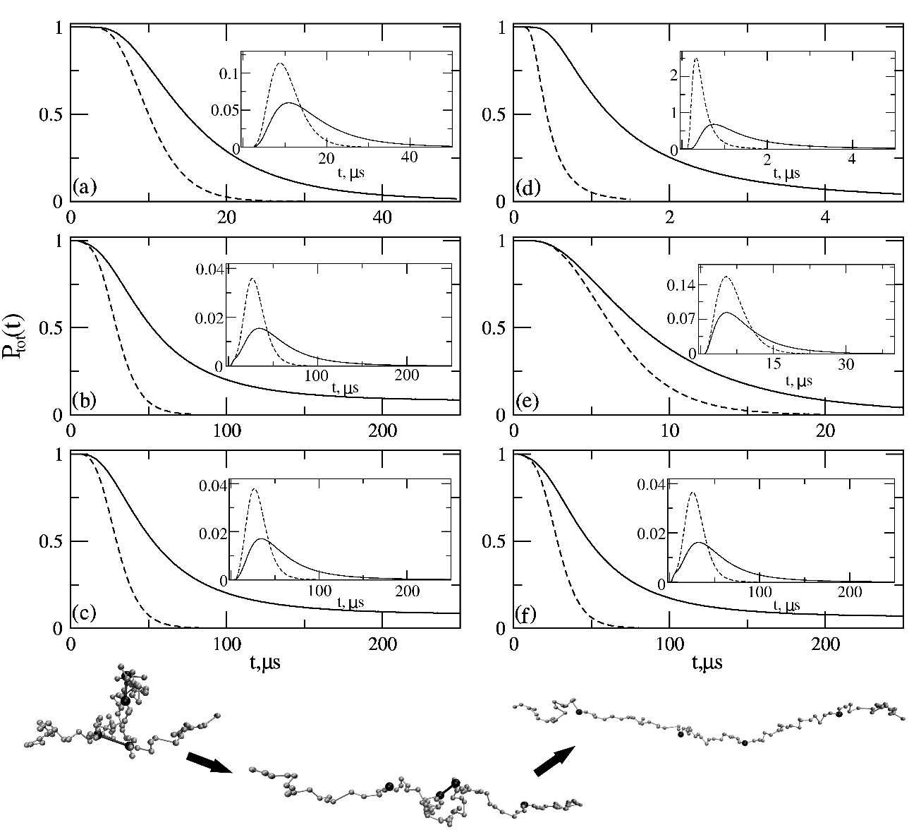
Figure 3: The survival probabilities $P_{tot}(t)$ for contact pairs $(1,100)$ and $(20,80)$ ($\bf{a}$), $(1,100)$ and $(40,60)$ ($\bf{b}$), and $(20,80)$ and $(40,60)$ ($\bf{c}$), $(1,100)$ and $(2,99)$ ($\bf{d}$), $(20,80)$ and $(21,79)$ ($\bf{e}$), and $(40,60)$ and $(41,59)$ ($\bf{f}$), for $f$$=$$40$pN (solid lines) and $80$pN (dashed lines), all with $\gamma$$=$$1$. The lifetime distributions $p_{tot}(t)$ are shown in the insets. Time scales vary greatly in all panels. Structures are for the intact pair $(20,80)$ $(40,60)$, disrupted contact $(20,80)$ and intact contact $(40,60)$, and both contacts disrupted are shown.

Plots of $P_{tot}(t)$ for two separated strong contacts at $f$$=$$40pN$ and $80pN$ show that, in general, increasing $f$ facilitates more rapid rupture of the binary contacts (Figs. 3a-3c). The presence of interior contacts delays their rupture (compare Figs. 3a with 3b and 3c) even though $f/f_{c}$$>$$1$. The time dependence of $P_{tot}(t)$ for two separated contacts (Figs 3a-c), after a lag phase, can be analyzed using two distinct exponential functions, which shows the rupture occurs by sequential kinetics, with $\{(r,s),(r^{\prime},s^{\prime}]\}$$\to$$\{(0),(r^{\prime},s^{\prime})\}$$\to$$\{(0),(0)]\}$. The rate limiting second step is the rupture of the more interior contact. Comparison of $P_{tot}(t)$, for $\gamma$$=$$1$ and $f$$=$$40pN$, for the nearest neighbor contact pairs $(r,s)$$=$$(1,100)$ and $(r^{\prime},s^{\prime})$$=$$(2,99)$, $(20,80)$ and $(21,79)$, and $(40,60)$ and $(41,59)$ (Fig. 3d-3f) with $P_{rs}(t)$ for single contact $(r,s)$$=$$(1,100)$, $(20,80)$, and $(40,60)$ (Fig. 1d-1f) shows that the double bond increases stability of the contact, especially for the interior contact $(40,60)$. The chain with double bonds ruptures in a single step, $\{(r,s),(r^{\prime},s^{\prime})\}$$\to$$\{(0),(0)\}$, i.e. the rip occurs cooperatively, so that $P_{tot}(t)$ decays with a single rate constant at long times. The decay of $P_{tot}(t)$ for separated contacts, $(r,s)$$=$$(20,80)$ and $(r^{\prime},s^{\prime})$$=$$(40,60)$, is slower than $P_{tot}(t)$ for the nearest neighbor contacts, $(1,100)$ and $(2,99)$ (Figs. 3c and 3d), and $P_{tot}^{eq}$ is larger, which shows that the persistence of binary interactions critically depends on the location of contacts in the chain. The lifetime distributions show that increasing the force from $f$$=$$40pN$ to $f$$=$$80pN$ results in the decreased stability of contacts and shorter lifetimes (Fig. 3). The contact lifetimes increase when they are located in the chain interior (Fig. 3). The lifetimes of the nearest neighbor contacts, $(1,100)$ and $(2,99)$ (Figs. 3d and 3e), are shorter than that for the pair, $(40,60)$ and $(41,59)$ (Fig. 3f), which shows the importance of the location of binary contacts with respect to the point of application of the force.

Conclusions: The present work shows that the shape of the free energy landscape can only be discerned by analyzing the topology-dependent lifetime distributions of adhesive contacts that reflect the structure the molecules. The continued increase in the temporal resolution in laser optical tweezer experiments should allow the prediction that, the internal motions of biomolecules are coupled to global fluctuations, to be tested. The present theory provides a conceptual framework for interpreting such experiments BlockAnnRevBiophys2007TinocoPNAS07FernandezPNAS07 . In contrast, the rich behavior predicted here cannot be obtained by solving for the dynamics in the exactly calculable equilibrium free energy profile in the presence of non-zero force. Accounting for the non-exponential distribution of unbinding lifetimes will require models that reflect the interplay between local chain motions and tension-induced global unfolding.

Acknowledgments: This work was supported by National Science Foundation Grant NSFCHE-05-14056.

References

(1)
W. J. Greenleaf, M. T. Woodside, S. M. Block, Annu. Rev. Biophys. Biomol. Struct.36, 171 (2007);
P. T. X. Li, C. Bustamante, and I. Tinoco, Jr., Proc. Natl. Acad. Sci. USA104, 7039 (2007);
K. A. Walther, F. Graeter, L. Dougan, C. L. Badilla, B. J. Berne, and J. M. Fernandez,
Proc. Natl. Acad. Sci. USA104, 7916 (2007).
(2)
C. Hyeon and D. Thirumalai, Proc. Natl. Acad. Sci. USA100, 10249 (2003);
O. K. Dudko, A. E. Filippov, J. Klafter, and M. Urbakh, Proc. Natl. Acad. Sci. USA100,
11378 (2003); O. K. Dudko, G. Hummer and A. Szabo, Phys. Rev. Lett.96, 108101 (2006).
(3)
V. Barsegov and D. Thirumalai, Phys. Rev. Lett.95, 168302 (2005).
(4)
C. Hyeon and D. Thirumalai, Biophys. J.90, 3410 (2006).
(5)
M. Doi and S. F. Edwards. The Theory of Polymer Dynamics, (Oxford University Press, New York, 1994).
(6)
P. Lancaster and M. Tismenetsky. Theory of Matrices, (Academic Press, Orlando, 1985);
H. V. Henderson and S. R. Searle. On Deriving the Inverse of a Sum of Matrices. SIAM Rev., 23,
53-60 (1981); M. P. Solf and T. A. Vilgis. J. Phys. A: Math. Gen, 28, 6655 (1995).
(7)
G. Casella and R. L. Berger. Statistical Inference, (Pacific Grove, Duxberry, 2002);
Davison, A. C. Statistical Models, (Cambridge University Press, Cambridge, 2003).
(8)
E. Bura, D. K. Klimov and V. Barsegov, Biophys. J.93, 1100 (2007); 94, 2516 (2008).
(9)
C. Hyeon, R. I. Dima and D. Thirumalai, Structure14, 1633 (2006).
(10)
E. J. Gumbel. Statistics of Extremes, (Dover Publications, New York, 2004).