Chaplygin inflation on the brane

Abstract

Brane inflationary universe model in the context of a Chaplygin gas equation of state is studied. General conditions for this model to be realizable are discussed. In the high-energy limit and by using a chaotic potential we describe in great details the characteristic of this model. The parameters of the model are restricted by using recent astronomical observations.

I Introduction

It is well known that inflation is to date the most compelling solution to many long-standing problems of the Big Bang model (horizon, flatness, monopoles, etc.) guth ; infla . One of the success of the inflationary universe model is that it provides a causal interpretation of the origin of the observed anisotropy of the cosmic microwave background (CMB) radiation, and also the distribution of large scale structures astro .

In concern to higher dimensional theories, implications of string/M-theory to Friedmann-Robertson-Walker (FRW) cosmological models have recently attracted great deal of attention, in particular, those related to brane-antibrane configurations such as space-like branessen1 . The realization that we may live on a so-called brane embedded in a higher-dimensional Universe has significant implications to cosmology 1 . In this scenario the standard model of particle is confined to the brane, while gravitations propagate in the bulk spacetimes. Since, the effect of the extra dimension induces additional terms in the Friedmann equation 22 ; 3 . One of the term that appears in this equation is a quadratic term in the energy density. Such a term generally makes it easier to obtain inflation in the early Universe 4 ; 5 . For a review, see, e.g., Ref.M .

On the other hand, the generalized Chaplygin gas has been proposed as an alternative model for describing the accelerating of the universe. The generalized Chaplygin gas is described by an exotic equation of state of the form Bento

$$p_{ch}=-\frac{A}{\rho_{ch}^{\beta}},$$ (1)

where $\rho_{ch}$ and $p_{ch}$ are the energy density and pressure of the generalized Chaplygin gas, respectively. $\beta$ is a constant that lies in the range $0<\beta\leq 1$, and $A$ is a positive constant. The original Chaplygin gas corresponds to the case $\beta=1$ 2 . Inserting this equation of state into the relativistic energy conservation equation leads to an energy density given by

$$\rho_{ch}=\left[A+\frac{B}{a^{3(1+\beta)}}\right]^{\frac{1}{1+\beta}},$$ (2)

where $a$ is the scale factor and $B$ is a positive integration constantBento .

The Chaplygin gas emerges as a effective fluid of a generalized d-brane in a (d+1, 1) space time, where the action can be written as a generalized Born-Infeld action Bento . These models have been extensively studied in the literature other . The parameters of the model were constrained using currents cosmological observations, such as, CMB CMB and supernova of type Ia (SNIa) SIa .

In the model of Chaplygin inspired inflation usually the scalar field, which drives inflation, is the standard inflaton field, where the energy density given by Eq.(2), can be extrapolate for obtaining a successful inflation period with a Chaplygin gas modelIc . Recently, tachyon-Chaplygin inflationary universe model was considered in yo , and the dynamics of the early universe and the initial conditions for inflation in a model with radiation and a Chaplygin gas was studied in Ref.Monerat:2007ud . As far as we know, a Chaplygin inspired inflationary model in which a brane-world model is considered has not been studied.

The motivation for introducing Chaplygin-brane scenarios is the increasing interest in higher-dimensional cosmological models, motivated by superstring theory, where the matter fields are confined to a lower-dimensional brane(related to open string modes), while gravity can propagate in the bulk (closed string modes). On the other hand, the Chaplygin gas model seems to be a viable alternative to models that provide an accelerated expansion of the early universe. Our aim is to quantify the modifications of the Chaplygin inspired inflation in the brane scenario. In order to do this we study the early universe dynamic and the cosmological perturbations in our model. We will show that these underlying assumptions allow for an inflationary scenario in which the observational constrains are successfully met.

The outline of the paper is a follows. The next section presents a short review of the modified Friedmann equation by using a Chaplygin gas, and we present the brane-Chaplygin inflationary model. Section III deals with the calculations of cosmological perturbations in general term. In Section IV we use a chaotic potential in the high-energy limit for obtaining explicit expression for the model. Finally, Sect.V summarizes our findings.

II The modified Friedmann equation and the brane-Chaplygin Inflationary phase.

We consider the five-dimensional brane scenario, in which the Friedmann equation is modified from its usual form, in the following way2 ; 3

$$H^{2}=\kappa\,\rho_{\phi}\left[1+\frac{\rho_{\phi}}{2\lambda}\right]+\frac{\Lambda_{4}}{3}+\frac{\xi}{a^{4}},$$ (3)

where $H=\dot{a}/a$ denotes the Hubble parameter, $\rho_{\phi}$ represents the matter confined to the brane, $\kappa=8\pi G/3=8\pi/3m_{p}^{2}$, $\Lambda_{4}$ is the four-dimensional cosmological constant and the final term represents the influence of bulk gravitons on the brane, where $\xi$ is an integration constant (this term appears as a form of dark radiation). The brane tension $\lambda$ relates the four and five-dimensional Planck masses via $m_{p}=\sqrt{3M_{5}^{6}/(4\pi\lambda)}$, and is constrained by the requirement of successful nucleosynthesis as $\lambda>$ (1MeV)⁴ Cline . We assume that the four-dimensional cosmological constant is set to zero, and once inflation begins the final term will rapidly become unimportant, leaving us withM

$$H^{2}=\kappa\left[A+\rho_{\phi}^{(1+\beta)}\right]^{\frac{1}{1+\beta}}\,\left[1+\frac{\left[A+\rho_{\phi}^{(1+\beta)}\right]^{\frac{1}{1+\beta}}}{2\lambda}\right].$$ (4)

Here, $\rho_{\phi}$ becomes $\rho_{\phi}=\frac{\dot{\phi}^{2}}{2}+V(\phi)$, and $V(\phi)=V$ is the scalar potential. Note that, in the low energy regime $[A+\rho_{\phi}^{(1+\beta)}]^{1/(1+\beta)}\ll\lambda$, the standard Chaplygin inflationary model is recovered, and in a very hight-energy regime, the contribution from the matter in Eq.(4) becomes proportional to $[A+\rho_{\phi}^{(1+\beta)}]^{2/(1+\beta)}$ in the effective energy density.

We assume that the scalar field is confined to the brane, so that its field equation has the standard form

$$\ddot{\phi}\,+3H\;\dot{\phi}+V^{\prime}=0,$$ (5)

where dots mean derivatives with respect to the cosmological time and $V^{\prime}=\partial V(\phi)/\partial\phi$. For convenience we will use units in which $c=\hbar=1$.

The modification of the Eq.(4) is realized from an extrapolation of Eq.(2), where the density matter $\rho_{m}\sim a^{-3}$ in introduced in such a way that we may write

$$\rho_{ch}=\left[A+\rho_{m}^{(1+\beta)}\right]^{\frac{1}{1+\beta}}\longrightarrow\left[A+\rho_{\phi}^{(1+\beta)}\right]^{\frac{1}{1+\beta}},$$ (6)

and thus, we identifying $\rho_{m}$ with the contributions of the scalar field which gives Eq.(4). The generalized Chaplygin gas model may be viewed as a modification of gravity, as described in Ref.Ber , and for chaotic inflation, in Ref.Ic . Different modifications of gravity have been proposed in the last few years, and there has been a lot of interest in the construction of early universe scenarios in higher-dimensional models motivated by string/M-theory Ran . It is well-known that these modifications can lead to important changes in the early universe. In the following we will take $\beta=1$ for simplicity, which means the usual Chaplygin gas.

During the inflationary epoch the energy density associated to the scalar field is of the order of the potential, i.e. $\rho_{\phi}\sim V$. Assuming the set of slow-roll conditions, i.e. $\dot{\phi}^{2}\ll V(\phi)$ and $\ddot{\phi}\ll 3H\dot{\phi}$, the Friedmann equation (4) reduces to

$$H^{2}\approx\kappa\,\sqrt{A+V^{2}}\left[1+\frac{\sqrt{A+V^{2}}}{2\lambda}\right],$$ (7)

and Eq. (5) becomes

$$3H\dot{\phi}\approx-V^{\prime}.$$ (8)

Introducing the dimensionless slow-roll parameters 4 , we write

$$\varepsilon=-\frac{\dot{H}}{H^{2}}\simeq\frac{m_{p}^{2}}{16\pi}\,\left[\frac{V\,V^{\prime 2}}{(A+V^{2})^{3/2}}\,\frac{\left(1+\frac{(A+V^{2})^{1/2}}{\lambda}\right)}{\left(1+\frac{(A+V^{2})^{1/2}}{2\lambda}\right)^{2}}\right],$$ (9)

and

$$\eta=-\frac{\ddot{\phi}}{H\,\dot{\phi}}\simeq\,\frac{m_{p}^{2}}{8\pi}\,\frac{V^{\prime\prime}}{(A+V^{2})^{1/2}}\,\left[1+\frac{(A+V^{2})^{1/2}}{2\lambda}\right]^{-1}.$$ (10)

Note that in the limit $A\rightarrow 0$, the slow-parameters $\varepsilon$ and $\eta$ coincides with brane-inflation 4 . Also, in the low-energy limit, $\sqrt{A+\rho_{\phi}^{2}}\ll\lambda$, the slow-parameters reduce to the standard form Ic .

The condition under which inflation takes place can be summarized with the parameter $\varepsilon$ satisfying the inequality $\varepsilon<1$, which is analogue to the requirement that $\ddot{a}>0$. This condition could be written in terms of the scalar potential and its derivative $V^{\prime}$, which becomes

$$V\,V^{\prime 2}\,\left[1+\frac{(A+V^{2})^{1/2}}{\lambda}\right]<\frac{16\pi}{m_{p}^{2}}\,(A+V^{2})^{3/2}\,\left[1+\frac{(A+V^{2})^{1/2}}{2\lambda}\right]^{2}.$$ (11)

Inflation ends when the universe heats up at a time when $\varepsilon\simeq 1$, which implies

$$V_{f}\,V_{f}^{\prime 2}\,\left[1+\frac{(A+V_{f}^{2})^{1/2}}{\lambda}\right]\simeq\frac{16\pi}{m_{p}^{2}}\,(A+V_{f}^{2})^{3/2}\,\left[1+\frac{(A+V_{f}^{2})^{1/2}}{2\lambda}\right]^{2}.$$ (12)

However, in the high-energy limit $[A+\rho_{\phi}^{2}]^{1/2}\approx[A+V^{2}]^{1/2}\gg\lambda$ Eq.(12) becomes

$$V_{f}^{\prime 2}\simeq\frac{4\pi}{m_{p}^{2}\,\lambda}\,\frac{(A+V_{f}^{2})^{2}}{V_{f}}.$$

The number of e-folds at the end of inflation is given by

$$N=-\frac{8\pi}{m_{p}^{2}}\,\int_{\phi_{*}}^{\phi_{f}}\frac{\sqrt{A+V^{2}}}{V^{\prime}}\,\left[1+\frac{\sqrt{A+V^{2}}}{2\lambda}\right]\,d\phi,$$ (13)

or equivalently

$$N=-\frac{8\pi}{m_{p}^{2}}\,\int_{V_{*}}^{V_{f}}\frac{\sqrt{A+V^{2}}}{V^{\prime 2}}\left[1+\frac{\sqrt{A+V^{2}}}{2\lambda}\right]\,d\,V.$$ (14)

Note that in the high-energy limit Eq.(14) becomes $N\simeq-(4\pi/m_{p}^{2}\lambda)\int_{V_{*}}^{V_{f}}\,[(A+V^{2})/V^{\prime 2}]dV$.

In the following, the subscripts $*$ and $f$ are used to denote the epoch when the cosmological scales exit the horizon and the end of inflation, respectively.

III Perturbations

In this section we will study the scalar and tensor perturbations for our model. It was shown in Ref. PB that the conservation of the curvature perturbation, $\cal{R}$, holds for adiabatic perturbations irrespective of the form of gravitational equations by considering the local conservation of the energy-momentum tensor. One has ${\cal{R}}=\psi+H\delta\phi/\dot{\phi}\simeq(H/\dot{\phi})(H/2\pi)$, where $\delta\phi$ is the perturbation of the scalar field $\phi$. For a scalar field the power spectrum of the curvature perturbations is given in the slow-roll approximation by following expression 4

$${\cal{P}_{R}}\simeq\left(\frac{H^{2}}{2\pi\dot{\phi}}\right)^{2}\,\simeq\,\frac{128\pi}{3m_{p}^{6}}\,\frac{(A+V^{2})^{3/2}}{V^{\prime 2}}\,\left[1+\frac{(A+V^{2})^{1/2}}{2\lambda}\right]^{3}.$$ (15)

Note that in the limit $A\rightarrow 0$ the amplitude of scalar perturbation given by Eq.(15) coincides with Ref.4 .

The scalar spectral index $n_{s}$ is given by $n_{s}-1=\frac{d\ln\,{\cal{P}_{R}}}{d\ln k}$, where the interval in wave number is related to the number of e-folds by the relation $d\ln k(\phi)=-dN(\phi)$. From Eq.(15), we get, $n_{s}\approx\,1\,-2(3\varepsilon-\eta)$, or equivalently

$$n_{s}\approx\,1\,-\frac{m_{p}^{2}}{8\pi}\,(A+V^{2})^{-1/2}\,\left[1+\frac{(A+V^{2})^{1/2}}{2\lambda}\right]^{-1}\,\left(\frac{3VV^{\prime}\,{}^{2}}{(A+V^{2})}\,\frac{\left[1+\frac{(A+V^{2})^{1/2}}{\lambda}\right]}{\left[1+\frac{(A+V^{2})^{1/2}}{2\lambda}\right]}-4V^{\prime\prime}\right).$$ (16)

One again, note that in the limit $A\rightarrow 0$, the scalar spectral index $n_{s}$ coincides with that corresponding to brane-world 4 .

One of the interesting features of the five-year data set from Wilkinson Microwave Anisotropy Probe (WMAP) is that it hints at a significant running in the scalar spectral index $dn_{s}/d\ln k=\alpha_{s}$ astro . From Eq.(16) we get that the running of the scalar spectral index becomes

$$\alpha_{s}=\left(\frac{4\,(A+V^{2})}{V\;V^{\prime}}\right)\,\left[\frac{\left(1+\frac{(A+V^{2})^{1/2}}{2\lambda}\right)}{\left(1+\frac{(A+V^{2})^{1/2}}{\lambda}\right)}\right]\;[3\,\varepsilon_{,\,\phi}-\eta_{,\,\phi}]\;\varepsilon.$$ (17)

In models with only scalar fluctuations the marginalized value for the derivative of the spectral index is approximately $-0.03$ from WMAP-five year data only 5 .

On the other hand, the generation of tensor perturbations during inflation would produce gravitational waves and this perturbations in cosmology are more involved since gravitons propagate in the bulk. The amplitude of tensor perturbations was evaluated in Ref.t

$${\cal{P}}_{g}=24\kappa\,\left(\frac{H}{2\pi}\right)^{2}\;F^{2}(x)\simeq\frac{6}{\pi^{2}}\,\kappa^{2}\,(A+V^{2})^{1/2}\,\left[1+\frac{(A+V^{2})^{1/2}}{2\lambda}\right]\,F^{2}(x),$$ (18)

where $x=Hm_{p}\sqrt{3/(4\pi\lambda)}$ and

$$F(x)=\left[\sqrt{1+x^{2}}-x^{2}\sinh^{-1}(1/x)\right]^{-1/2}.$$

Here the function $F(x)$ appeared from the normalization of a zero-mode. The spectral index $n_{g}$ is given by $n_{g}=\frac{d{\cal{P}}_{g}}{d\,\ln k}=-\frac{2x_{,\,\phi}}{N_{,\,\phi}\,x}\frac{F^{2}}{\sqrt{1+x^{2}}}$.

From expressions (15) and (18) we write the tensor-scalar ratio as

$$r(k)=\left.\left(\frac{{\cal{P}}_{g}}{P_{\cal R}}\right)\right|_{k=k_{*}}\simeq\left.\left(\frac{8}{3\,\kappa}\,\frac{V^{\prime 2}\;F^{2}(V)}{(A+V^{2})\;[1+(A+V^{2})^{1/2}/2\lambda]}\right)\right|_{\,k=k_{*}}.$$ (19)

Here, $k_{*}$ is referred to $k=Ha$, the value when the universe scale crosses the Hubble horizon during inflation.

Combining WMAP five-year dataastro with the Sloan Digital Sky Survey (SDSS) large scale structure surveys Teg , it is found an upper bound for $r$ given by $r(k_{*}\simeq$ 0.002 Mpc^-1)$<0.28\,(95\%CL)$, where $k_{*}\simeq$0.002 Mpc^-1 corresponds to $l=\tau_{0}k\simeq 30$, with the distance to the decoupling surface $\tau_{0}$= 14,400 Mpc. The SDSS measures galaxy distributions at red-shifts $a\sim 0.1$ and probes $k$ in the range 0.016 $h$ Mpc^-1$<k<$0.011 $h$ Mpc^-1. The recent WMAP five-year results give the values for the scalar curvature spectrum $P_{\cal R}(k_{*})\simeq 2.4\times\,10^{-9}$ and the scalar-tensor ratio $r(k_{*})=0.055$. We will make use of these values to set constrains on the parameters of the model.

IV Chaotic potential in the high-energy limit.

Let us consider an inflaton scalar field $\phi$ with a chaotic potential. We write for the chaotic potential $V=m^{2}\phi^{2}/2$, where $m$ is the mass of the scalar field. An estimation of this parameter is given for Chaplygin standard inflation in Ref.Ic . In the following, we develop models in the high-energy limit, i.e. $\sqrt{A+V^{2}}\gg\lambda$.

From Eq.(14) the number of e-folds results in

$$N=\frac{2\pi}{\lambda\,m^{2}\,m_{p}^{2}}\;[h(V_{*})-h(V_{f})],$$ (20)

where

$$h(V)=\frac{V^{2}}{2}+A\;\ln V.$$ (21)

On the other hand, we may establish that the end of inflation is governed by the condition $\varepsilon=1$, from which we get that the square of the scalar potential becomes

$$V(\phi=\phi_{f})=V_{f}=\frac{1}{2\sqrt{2\pi}}\;\left[m\,m_{p}\,\sqrt{\lambda}+\sqrt{\lambda\,m^{2}\,m_{p}^{2}-8\pi\,A}\right].$$ (22)

Note that in the limit $A\rightarrow 0$ we obtain $V_{f}\sim m\,\sqrt{\lambda}\,m_{p}$, which coincides with that reported in Ref.4 .

From Eq.(15) we obtain that the scalar power spectrum is given by

$$P_{\cal R}(k)\approx\;\frac{8\pi}{3\,m_{p}^{6}}\,\frac{1}{m^{2}\,\lambda^{3}}\left[\frac{(A+V^{2})^{3}}{V}\right],$$ (23)

and from Eq.(19) the tensor-scalar ratio becomes

$$r(k)\approx\;\frac{4\,m_{p}^{2}\,\lambda\,m^{2}}{\pi}\left[\frac{V}{(A+V^{2})^{3/2}}\,F^{2}(V)\right].$$ (24)

By using, that $V^{\prime}\,{}^{2}=2\,m^{2}\,V$, we obtain from Eq.(16)

$$n_{s}-1=-\frac{m_{p}^{2}}{2\pi}\,\frac{\lambda\,m^{2}}{(A+V^{2})}\left[\frac{3\,V^{2}}{(A+V^{2})}-2\right],$$ (25)

and from Eq.(17) that

$$\alpha_{s}\simeq-\frac{m_{p}^{4}\,m^{4}\,\lambda^{2}}{2\pi^{2}}\,\left[\frac{5V^{2}-7A}{(A+V^{2})^{4}}\right]\,V^{2}.$$ (26)

The Eqs.(23) and (25) has roots that can be solved analytically for the parameters $m$ and $A$, as a function of $n_{s}$, $P_{\cal R}$, $V$ and $\lambda$. The real root solution for $m^{2}$, and $A$ becomes

$$m^{2}=\left(\frac{\pi}{4\,P_{\cal R}\,\lambda^{3}\,m_{p}^{6}}\right)\,\left[\frac{3\,V}{2}\left(3V^{4}+\Im\right)+\sqrt{\Im}\left[6V^{3}+(n_{s}-1)P_{\cal R}\lambda^{2}\,m_{p}^{4}\right]\right],$$ (27)

and

$$A=\frac{1}{4}\left(\sqrt{\Im}-V^{2}\right)$$ (28)

where

$$\Im=9V^{4}+6(n_{s}-1)P_{\cal R}\,V\,\lambda^{2}\,m_{p}^{4}$$

From Eq.(28) and since $A>0$, the ratio $V^{3}/\lambda^{2}$ satisfies the inequality $V^{3}/\lambda^{2}>3(1-ns)P_{\cal R}\,m_{p}^{4}/4$. This inequality allows us to obtain an lower limit for the ratio $V^{3}(\phi)/\lambda^{2}$ evaluate when the cosmological scales exit the horizon, i.e. $V_{*}^{3}/\lambda^{2}>7.2\times 10^{-11}m_{p}^{4}$. Here, we have used the WMAP five year data where $P_{\cal R}(k_{*})\simeq 2.4\times 10^{-9}$ and $n_{s}(k_{*})\simeq 0.96$.

Note that in the limit $A\rightarrow 0$, the constrains $m\approx 10^{-5}M_{5}$ and $V_{*}=m^{2}\phi_{*}^{2}/2\approx 10^{-4}M_{5}^{4}$ are recovered 4 . Here, we used the relation $m_{p}=M_{5}^{3}\,\sqrt{3/(4\pi\lambda)}$.

In Fig. 1 we have plotted the adimensional quantity $\lambda^{2}/m_{p}^{8}$ versus the adimensional scalar potential evaluated when the cosmological scales exist the horizon $V_{*}/m_{p}^{4}$. In doing this, we used Eq.(26) that has roos that can be solved for the brane tension $\lambda$, as a function of $\alpha_{s}$, $m$, $A$ and $V$. For a real root solution for $\lambda$, and from Eqs. (27) and (28) we obtain a relation of the form $\lambda=f(V_{*})$ for a fixed values of $\alpha_{s}$, $n_{s}$ and $P_{\cal R}$. In this plot we using the WMAP five year data where $P_{\cal R}(k_{*})\simeq 2.4\times 10^{-9}$, $n_{s}(k_{*})\simeq 0.96$, $\alpha_{s}(k_{*})\simeq-0.03$. In Fig. 2 we have plotted the tensor-scalar ratio given by Eq.(24) versus the adimentional parameter $A/m_{p}^{4}$. The WMAP five-year data favors the tensor-scalar ratio $r\simeq 0.055$ and the from Fig. 2 we obtain that $A$ parameter becomes $A\simeq 4\times 10^{-13}m_{p}^{8}$. For this value for $A$ parameter we get the values $V_{*}=4\times 10^{-7}m_{p}^{4}$, $\lambda\simeq 2\times 10^{-8}m_{p}^{4}$, and $m\simeq 10^{-5}m_{p}$. Also, the number of e-folds, $N$, becomes of the order of $N\sim 55$. We should note also that the $A$ parameter becomes large by two order of magnitude and the $m$ parameter becomes similar when it is compared with the case of Chaplygin inflation in the low-energy limitIc .

On the other hand, is interesting to compare the role that brane effects play in our model, with the one they play in the context of tachyonic inflation x . In doing this, we using the above parameters, i.e. $\lambda\simeq 2\times 10^{-8}m_{p}^{4}$ and $V_{*}=4\times 10^{-7}m_{p}^{4}$ which correspond to the five-dimensional Planck mass, $M_{5}\simeq 6.6\times 10^{-2}m_{p}$ and $\phi_{*}\simeq 89m_{p}$. Here, we used the relations $m_{p}=M_{5}^{3}\,\sqrt{3/(4\pi\lambda)}$, $V_{*}=m^{2}\phi_{*}^{2}/2$ and $m\sim 10^{-5}m_{p}$. We should note that $M_{5}$ becomes similar and the $\phi_{*}$ scalar field becomes large by two order of magnitude when it is compared with the case of tachyonic inflation. In addition, the number of e-folds, $N$, is smaller than the reported in tachyon inflation.

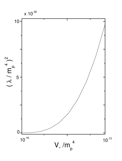
Figure 1: The plot shows the adimentional square of the brane tension $(\lambda/m_{p}^{4})^{2}$ versus the adimentional scalar potential $V_{*}/m_{p}^{4}$. Here, we have used the WMAP five-year data where $P_{\cal R}(k_{*})\simeq 2.4\times 10^{-9}$, $n_{s}(k_{*})\simeq 0.96$ and $\alpha_{s}(k_{*})\simeq-0.03$.

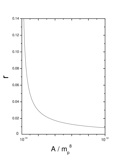
Figure 2: The plot shows the tensor-scalar ratio $r$ versus the adimentional parameter $A/m_{p}^{8}$. Here, we have used the WMAP five-year data where $P_{\cal R}(k_{*})\simeq 2.4\times 10^{-9}$, $n_{s}(k_{*})\simeq 0.96$ and $\alpha_{s}(k_{*})\simeq-0.03$.

V Conclusions

In this paper we have studied the brane-Chaplygin inflationary model. In the slow-roll approximation we have found a general relation between the scalar potential and its derivative. This has led us to a general criterium for inflation to occur (see Eq.(11)). We have also obtained explicit expressions for the corresponding scalar spectrum index $n_{s}$ and its running $\alpha_{s}$.

By using a chaotic potential in the high-energy regime and from the WMAP five year data, we found the constraints of the parameter $A$ from the tensor-scalar ratio $r$ (see Fig. 2). In order to bring some explicit results we have taken the constraints $A\simeq 10^{-13}m_{p}^{8}$, from which we get the values $V_{*}\simeq 3\times 10^{-7}m_{p}^{4}$, $\lambda\simeq 2\times 10^{-8}m_{p}^{4}$ and $m\simeq 10^{-5}m_{p}$. Here, we have used the WMAP five year data where $P_{\cal R}(k_{*})\simeq 2.4\times 10^{-9}$, $n_{s}(k_{*})\simeq 0.96$, $\alpha_{s}(k_{*})\simeq-0.03$ and $r(k_{*})\simeq 0.055$. Note that the restrictions imposed by currents observational data allowed us to establish a small range for the parameters that appear in the brane-Chaplygin inflationary model.

We have not addressed reheating and transition to standard cosmology in our model (see e.g., Ref.u ). However, a more accurate calculation for the reheating temperature in the hight-energy scenario, would be necessary for establishing some constrains on the parameters of the model. We hope to return to this point in the near future.

- (1) A. Guth, Phys. Rev. D 23, 347 (1981).
- (2) A. Albrecht and P. J. Steinhardt, Phys. Rev. Lett. 48, 1220 (1982); A complete description of inflationary scenarios can be found in the book by A. Linde , Particle physics and inflationary cosmology (Gordon and Breach, New York, 1990).
- (3) J. Dunkley et al. [WMAP Collaboration], arXiv:0803.0586 [astro-ph]; G. Hinshaw et al., arXiv:0803.0732 [astro-ph].
- (4) A. Sen, JHEP 0204, 048 (2002).
- (5) K. Akama, Lect. Notes Phys. 176, 267 (1982); V. A. Rubakov and M. E. Shaposhnikov, Phys. Lett. B 159, 22 (1985); N. Arkani- Hamed, S. Dimopoulos, and G. Dvali, Phys. Lett. B 429, 263 (1998); M. Gogberashvili, Europhys. Lett. 49, 396 (2000); L. Randall and R. Sundrum, Phys. Rev. Lett. 83, 3370 (1999); 83, 4690 (1999).
- (6) P. Bin etruy, C. Deffayet, and D. Langlois, Nucl. Phys. B565, 269 (2000) ; P. Bin etruy, C. Deffayet, U. Ellwanger, and D. Langlois, Phys. Lett. B 477, 285 (2000).
- (7) T. Shiromizu, K. Maeda, and M. Sasaki, Phys. Rev. D 62, 024012 (2000).
- (8) R. Maartens, D. Wands, B. A. Bassett, and I. P. C. Heard, Phys. Rev. D 62, 041301 (2000).
- (9) J. M. Cline, C. Grojean, and G. Servant, Phys. Rev. Lett.83, 4245 (1999); C. C saki, M. Graesser, C. Kolda, and J. Terning, Phys. Lett. B 462, 34 (1999); D. Ida, JHEP 0009, 014 (2000); R. N. Mohapatra, A. P erez-Lorenzana, and C. A. de S. Pires, Phys. Rev. D 62, 105030 (2000); R. N. Mohapatra, A. P erez-Lorenzana, and C. A. de S. Pires, Int. J. Mod. Phys. A 16, 1431 (2001); Y. Gong, arXiv:gr-qc/0005075.
- (10) R. Maartens, arXiv:gr-qc/0101059.
- (11) M. C. Bento, O. Bertolami and A. Sen, Phys. Rev. D 66, 043507 (2002).
- (12) A. Kamenshchik, U. Moschella and V. Pasquier, Phys. Lett. B 511, 265 (2001); N. Bilic, G. B. Tupper and R. D. Viollier, Phys. Lett. B 535, 17 (2002).
- (13) H. B. Benaoum, arXiv:hep-th/0205140; A. Dev, J.S. Alcaniz and D. Jain, Phys. Rev. D 67 023515 (2003); G. M. Kremer, Gen. Rel. Grav. 35, 1459 (2003); R. Bean, O. Dore, Phys. Rev. D 68, 023515 (2003); Z.H. Zhu, Astron. Astrophys. 423, 421 (2004); H. Sandvik, M. Tegmark, M. Zaldarriaga and I. Waga, Phys. Rev. D 69, 123524 (2004) ; L. Amendola, I. Waga and F. Finelli, JCAP 0511, 009 (2005); P.F. Gonzalez-Diaz, Phys. Lett. B 562, 1 (2003) ; L.P. Chimento, Phys. Rev. D 69, 123517 (2004); L.P. Chimento and R. Lazkoz, Phys. Lett. B 615, 146 (2005); U. Debnath, A. Banerjee and S. Chakraborty, Class. Quant. Grav. 21, 5609 (2004); W. Zimdahl and J.C. Fabris, Class. Quant. Grav. 22, 4311 (2005); P. Wu and H. Yu,Class. Quant. Grav. 24, 4661 (2007); M. R. Setare, Phys. Lett. B 654, 1 (2007); M. Bouhmadi-Lopez and R. Lazkoz, Phys. Lett. B 654, 51 (2007).
- (14) M.C. Bento, O. Bertolami and A. Sen, Phys. Lett. B 575, 172 (2003); M.C. Bento, O. Bertolami and A.A. Sen, Phys. Rev. D67, 063003 (2003).
- (15) M. Makler, S.Q. de Oliveira and I. Waga, Phys. Lett. B 555, 1 (2003); J.C. Fabris, S.V.B. Goncalves and P.E. de Souza, arXiv:astro-ph/0207430; M. Biesiada, W. Godlowski and M. Szydlowski, Astrophys. J. 622, 28 (2005); Y. Gong and C.K. Duan, Mon. Not. Roy. Astron. Soc. 352, 847 (2004); Y. Gong, JCAP 0503, 007 (2005) .
- (16) O. Bertolami and V. Duvvuri, Phys. Lett. B 640, 121 (2006).
- (17) S. del Campo and R. Herrera, Phys. Lett. B 660, 282 (2008).
- (18) G. A. Monerat et al., Phys. Rev. D 76, 024017 (2007).
- (19) J. M. Cline, C. Grojean and G. Servant, Phys. Rev. Lett. 83, 4245 (1999)
- (20) T. Barreiro, A.A. Sen, Phys. Rev. D 70, 124013 (2004).
- (21) L. Randall and R. Sundrum, Phys. Rev. Lett. 83, 4690 (1999); T. Shiromizu, K. Maeda and M. Sasaki, Phys. Rev. D 62, 024012 (2000); D. Dvali, G. Gabadadze and M. Porrati, Phys.Lett. B 485, 208 (2000); K. Freese and M. Lewis, Phys. Lett. B 540, 1 (2002); R. Maartens, Lect. Notes Phys. 653 213 (2004); A. Lue, Phys. Rept. 423, 1 (2006).
- (22) M. Fairbairn and M. H. G. Tytgat, Phys. Lett. B 546, 1 (2002).
- (23) S. Tsujikawa, D. Parkinson and B. A. Bassett, Phys. Rev. D 67, 083516 (2003).
- (24) D. Langlois, R. Maartens and D. Wands, Phys. Lett. B 489, 259 (2000).
- (25) M. Tegmark et al., Phys. Rev. D 69, 103501 (2004).
- (26) M. C. Bento, O. Bertolami and A. A. Sen, Phys. Rev. D 67, 063511 (2003).
- (27) E. J. Copeland, A. R. Liddle and J. E. Lidsey, Phys. Rev. D 64, 023509 (2001); E. J. Copeland and O. Seto, Phys. Rev. D 72, 023506 (2005).