Recent results on rare decay $\pi^{0}\rightarrow e^{+}e^{-}$

Abstract

Experimental and theoretical progress concerning the rare decay $\pi^{0}\rightarrow e^{+}e^{-}$ is briefly reviewed. It includes the latest data from KTeV and a new model independent estimate of the decay branching which show the deviation between experiment and theory at the level of $3.3\sigma$.

1 Introduction

Astrophysics observables tell us that $95\%$ of the matter in the Universe is not described in terms of the Standard Model (SM) matter. Thus, the search for the traces of New Physics is a fundamental problem of particle physics. There are two strategies to look for the effects of New Physics: experiments at high energy and experiments at low energy. In high-energy experiments it is considered that due to a huge amount of energy the heavy degrees of freedom presumably characteristic of the SM extension sector are possible to excite. In low-energy experiments it is huge statistics that compensates the lack of energy by measuring the rare processes characteristic of such extensions. At present, there is no any evidence for deviation of SM predictions from the results of high-energy experiments and we are waiting for the LHC epoch. On the other hand, in low-energy experiments there are rough edges indicating such deviations. The most famous example is the muon $(g-2)$. Below it will be shown that due to recent experimental and theoretical progress the rare process $\pi^{0}\rightarrow e^{+}e^{-}$ became a good SM test process and that at the moment there is a discrepancy between the SM prediction and experiment at the level of $3.3\sigma$ deviation.

2 KTeV data

In 2007, the KTeV collaboration published the result [1] for the branching ratio of the pion decay into an electron-positron pair

$$B_{\mathrm{no-rad}}^{\mathrm{KTeV}}\left(\pi^{0}\rightarrow e^{+}e^{-}\right)=\left(7.48\pm 0.38\right)\cdot 10^{-8}.$$ (1)

The result is based on observation of 794 candidate $\pi^{0}\rightarrow e^{+}e^{-}$ events using $K_{L}\rightarrow 3\pi^{0}$ as a source of tagged $\pi^{0}$s. Due to a complicated chain of the process and a good technique for final state resolution used by KTeV this is a process with low background.

3 Classical theory of $\pi^{0}\rightarrow e^{+}e^{-}$ decay

The rare decay $\pi^{0}\rightarrow e^{+}e^{-}$ has been studied theoretically over the years, starting with the first prediction of the rate by Drell [2]. Since no spinless current coupling of quarks to leptons exists, the decay is described in the lowest order of QED as a one-loop process via the two-photon intermediate state, as shown in Fig. 1. A factor of $2\left(m_{e}/m_{\pi}\right)^{2}$ corresponding to the approximate helicity conservation of the interaction and two orders of $\alpha$ suppress the decay with respect to the $\pi^{0}\rightarrow\gamma\gamma$ decay, leading to an expected branching ratio of about $10^{-7}$. In the Standard Model contributions from the weak interaction to this process are many orders of magnitude smaller and can be neglected.

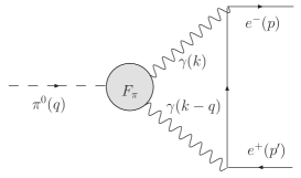
Figure 1: Triangle diagram for the $\pi^{0}\rightarrow e^{+}e^{-}$ process with a pion $\pi^{0}\rightarrow\gamma^{\ast}\gamma^{\ast}$ form factor in the vertex.

To the lowest order in QED the normalized branching ratio is given by

$$R\left(\pi^{0}\rightarrow e^{+}e^{-}\right)=\frac{B\left(\pi^{0}\rightarrow e^{+}e^{-}\right)}{B\left(\pi^{0}\rightarrow\gamma\gamma\right)}$$ (2)

$$\ =2\left(\frac{\alpha}{\pi}\frac{m_{e}}{m_{\pi}}\right)^{2}\beta_{e}\left(m_{\pi}^{2}\right)\left|\mathcal{A}\left(m_{\pi}^{2}\right)\right|^{2},$$

where $\beta_{e}\left(q^{2}\right)=\sqrt{1-4\frac{m_{e}^{2}}{q^{2}}}$, $B\left(\pi^{0}\rightarrow\gamma\gamma\right)=0.988$. The amplitude $\mathcal{A}$ can be written as

$$\mathcal{A}\left(q^{2}\right)=\frac{2i}{q^{2}}\int\frac{d^{4}k}{\pi^{2}}F_{\pi\gamma^{\ast}\gamma^{\ast}}\left(k^{2},\left(k-q\right)^{2}\right)$$ (3)

$$\cdot\frac{q^{2}k^{2}-\left(qk\right)^{2}}{\left(k^{2}+i\varepsilon\right)\left(\left(k-q\right)^{2}+i\varepsilon\right)\left(\left(k-p\right)^{2}-m_{e}^{2}+i\varepsilon\right)},$$

where $q^{2}=m_{\pi}^{2},p^{2}=m_{e}^{2}$. $F_{\pi\gamma^{\ast}\gamma^{\ast}}$ is the form factor of the transition $\pi^{0}\rightarrow\gamma^{\ast}\gamma^{\ast}$ with off-shell photons.

The imaginary part of $\mathcal{A}$ is defined uniquely as

$$\mathrm{Im}\mathcal{A}\left(q^{2}\right)=\frac{\pi}{2\beta_{e}\left(q^{2}\right)}\ln\left(y_{e}\left(q^{2}\right)\right),$$ (4)

$$y_{e}\left(q^{2}\right)=\frac{1-\beta_{e}\left(q^{2}\right)}{1+\beta_{e}\left(q^{2}\right)}.$$

It comes from the contribution of real photons in the intermediate state and is model independent since $F_{\pi\gamma^{\ast}\gamma^{\ast}}\left(0,0\right)=1$. Using inequality $\left|\mathcal{A}\right|^{2}\geq\left(\mathrm{Im}\mathcal{A}\right)^{2}$ one can get the well-known unitary bound for the branching ratio [3]

$$B\left(\pi^{0}\rightarrow e^{+}e^{-}\right)$$ (5)

$$\geq B^{\mathrm{unitary}}\left(\pi^{0}\rightarrow e^{+}e^{-}\right)=4.69\cdot 10^{-8}.$$

One can attempt to reconstruct the full amplitude by using a once-subtracted dispersion relation [5]

$$\mathcal{A}\left(q^{2}\right)=\mathcal{A}\left(q^{2}=0\right)+\frac{q^{2}}{\pi}\int_{0}^{\infty}ds\frac{\mathrm{Im}\mathcal{A}\left(s\right)}{s\left(s-q^{2}\right)}.$$ (6)

If one assumes that Eq. (4) is valid for any $q^{2}$, then one arrives for $q^{2}\geq 4m_{e}^{2}$ at [6, 7, 8]

$$\mathrm{Re}\mathcal{A}\left(q^{2}\right)=\mathcal{A}\left(q^{2}=0\right)+\frac{1}{\beta_{e}\left(q^{2}\right)}$$ (7)

$$\cdot\left[\frac{1}{4}\ln^{2}\left(y_{e}\left(q^{2}\right)\right)+\frac{\pi^{2}}{12}+\mathrm{Li}_{2}\left(-y_{e}\left(q^{2}\right)\right)\right],$$

where $\mathrm{Li}_{2}\left(z\right)=-\int_{0}^{z}\left(dt/t\right)\ln\left(1-t\right)$ is the dilogarithm function. The second term in Eq. (7) takes into account a strong $q^{2}$ dependence of the amplitude around the point $q^{2}=0$ occurring due to the branch cut coming from the two-photon intermediate state. In the leading order in $\left(m_{e}/m_{\pi}\right)^{2},$ Eq. (7) reduces to

$$\mathrm{Re}\mathcal{A}\left(m_{\pi}^{2}\right)=\mathcal{A}\left(q^{2}=0\right)+\ln^{2}\left(\frac{m_{e}}{m_{\pi}}\right)+\frac{\pi^{2}}{12}.$$ (8)

Thus, the amplitude is fully reconstructed up to a subtraction constant. Usually, this constant containing the nontrivial dynamics of the process is calculated within different models describing the form factor $F_{\pi}(k^{2},q^{2})$ [4, 5, 7, 9, 10]. However, it has recently been shown in [10] that this constant may be expressed in terms of the inverse moment of the pion transition form factor given in symmetric kinematics of spacelike photons

$$\mathcal{A}\left(q^{2}=0\right)=3\ln\left(\frac{m_{e}}{\mu}\right)-\frac{5}{4}$$ (9)

$$-\frac{3}{2}\left[\int_{0}^{\mu^{2}}dt\frac{F_{\pi\gamma^{\ast}\gamma^{\ast}}\left(t,t\right)-1}{t}\right.$$

$$+\left.\int_{\mu^{2}}^{\infty}dt\frac{F_{\pi\gamma^{\ast}\gamma^{\ast}}\left(t,t\right)}{t}\right].$$

Here, $\mu$ is an arbitrary (factorization) scale. One has to note that the logarithmic dependence of the first term on $\mu$ is compensated by the scale dependence of the integrals in the brackets. In this way two independent processes becomes related.

4 Importance of CLEO data on $F_{\pi\gamma^{\ast}\gamma}$

In order to estimate the integral in Eq. (9), one needs to define the pion transition form factor in symmetric kinematics for spacelike photon momenta. Since it is unknown from the first principles, we will adapt the available experimental data to perform such estimates. Let us first use the fact that $F_{\pi\gamma^{\ast}\gamma^{\ast}}\left(t,t\right)<F_{\pi\gamma^{\ast}\gamma^{\ast}}\left(t,0\right)$ for $t>0$ in order to obtain the lower bound of the integral in Eq. (9). For this purpose, we take the experimental results from the CELLO [11] and CLEO [12] Collaborations for the pion transition form factor in asymmetric kinematics for spacelike photon momentum which is well parametrized by the monopole form [12]

$$F_{\pi\gamma^{\ast}\gamma^{\ast}}^{\mathrm{CLEO}}\left(t,0\right)=\frac{1}{1+t/s_{0}^{\mathrm{CLEO}}},$$ (10)

$$s_{0}^{\mathrm{CLEO}}=\left(776\pm 22\quad\mathrm{MeV}\right)^{2}.$$

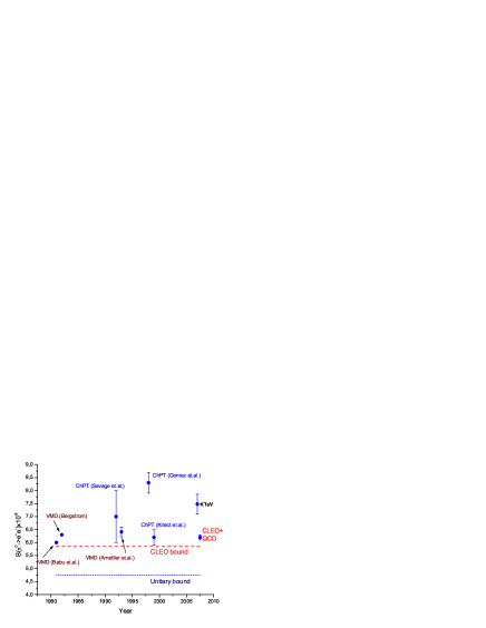
Figure 2: Evolution of model predictions and comparison with the latest KTeV result.

For this type of the form factor one finds from Eq. (9) that

$$\mathcal{A}\left(q^{2}=0\right)$$ (11)

$$>-\frac{3}{2}\ln\left(\frac{s_{0}^{\mathrm{CLEO}}}{m_{e}^{2}}\right)-\frac{5}{4}=-23.2\pm 0.1.$$

Thus, for the branching ratio we are able to establish the important lower bound which considerably improves the unitary bound given by Eq. (5)

$$B\left(\pi^{0}\rightarrow e^{+}e^{-}\right)$$ (12)

$$>B^{\mathrm{CLEO}}\left(\pi^{0}\rightarrow e^{+}e^{-}\right)=\left(5.84\pm 0.02\right)\cdot 10^{-8}.$$

It is natural to assume that the monopole form is also a good parametrization for the form factor in symmetric kinematics

$$F_{\pi\gamma^{\ast}\gamma^{\ast}}\left(t,t\right)=\frac{1}{1+t/s_{1}}.$$ (13)

The scale $s_{1}$ can be fixed from the relation for the slopes of the form factors in symmetric and asymmetric kinematics at low $t$ [13],

$$\left.-\frac{\partial F_{\pi\gamma^{\ast}\gamma^{\ast}}\left(t,t\right)}{\partial t}\right|_{t=0}=\left.-2\frac{\partial F_{\pi\gamma^{\ast}\gamma^{\ast}}\left(t,0\right)}{\partial t}\right|_{t=0},$$ (14)

that gives $s_{1}=s_{0}/2$. Note that a similar reduction of the scale is also predicted by OPE QCD from the large momentum behavior of the form factors: $s_{1}^{OPE}=s_{0}^{OPE}/3$ [14]. Thus, the estimate for $\mathcal{A}\left(0\right)$ can be obtained from Eq. (11) by shifting the lower bound by a positive number which belongs to the interval $[3\ln(2)/2,3\ln(3)/2]$

$$\mathcal{A}\left(q^{2}=0\right)=-\frac{3}{2}\ln\left(\frac{s_{1}}{m_{e}^{2}}\right)-\frac{5}{4}=-21.9\pm 0.3.$$ (15)

With this result the branching ratio becomes

$$B\left(\pi^{0}\rightarrow e^{+}e^{-}\right)=\left(6.23\pm 0.09\right)\cdot 10^{-8}.$$ (16)

This is $3.3$ standard deviations lower than the KTeV result given by Eq. (1).

5 Other decay modes

The $\eta\rightarrow l^{+}l^{-}$ decay can be analyzed in a similar manner. As in the pion case, the CLEO Collaboration has parametrized the data for the $\eta$-meson in the monopole form [12]:

$$F_{\eta\gamma^{\ast}\gamma^{\ast}}^{\mathrm{CLEO}}\left(t,0\right)=\frac{1}{1+t/s_{0\eta}^{\mathrm{CLEO}}},$$ (17)

$$s_{0\eta}^{\mathrm{CLEO}}=\left(774\pm 29\quad\mathrm{MeV}\right)^{2},$$

which is very close to the relevant pion parameter. Then following the previous case (with evident substitutions), one finds the bounds for the $q^{2}\rightarrow 0$ limit of the amplitude $\eta\rightarrow\mu^{+}\mu^{-}$ as

$$\mathcal{A}_{\eta}\left(q^{2}=0\right)$$ (18)

$$>-\frac{3}{2}\ln\left(\frac{s_{0\eta}^{\mathrm{CLEO}}}{m_{\mu}^{2}}\right)-\frac{5}{4}=-\left(7.2\pm 0.1\right),$$

and for $\eta\rightarrow e^{+}e^{-}$ one gets again Eq. (11). The obtained estimates allow one to find the bounds for the branching ratios

$$B\left(\eta\rightarrow\mu^{+}\mu^{-}\right)<\left(6.23\pm 0.12\right)\cdot 10^{-6},$$ (19)

$$B\left(\eta\rightarrow e^{+}e^{-}\right)>\left(4.33\pm 0.02\right)\cdot 10^{-9}.$$

It is important to note that for the decay $\eta\rightarrow\mu^{+}\mu^{-}$ we get the upper limit for the branching. This is because the real part of the amplitude for this process taken at the physical point $q^{2}=m_{\eta}^{2}$ for the parameter $s_{0\eta}^{\mathrm{CLEO}}$ remains negative and a positive shift due to the change of the scale $s_{0\eta}\rightarrow s_{1\eta}$ reduces the absolute value of the real part of the amplitude $\left|\mathrm{Re}\mathcal{A}\left(m_{\eta}^{2}\right)\right|$. At the same time, considering the decays of $\pi^{0}$ and $\eta$ into an electron-positron pair, the evolution to physical point (7) makes the real part of the amplitude to be positive for the parameter $s_{0}^{\mathrm{CLEO}}$ and the absolute value of the real part of the amplitude increases in changing the scales of the meson form factors. Thus, it would be very interesting to check experimentally the predicted bounds for the process $\eta\rightarrow\mu^{+}\mu^{-}$.

The predictions for the decays $\eta\rightarrow l^{+}l^{-}$ obtained by reducing the scale $s_{0\eta}^{\mathrm{CLEO}}\rightarrow s_{1\eta}$ for the case of the $\eta$-meson transition form factor are given in Table 1. Also note the recent measurement by the WASA/Celcius Collaboration [15] which improves the upper limit for the branching $\eta\rightarrow e^{+}e^{-}$.

Table 1: Values of the branchings $B\left(P\rightarrow l^{+}l^{-}\right)$ obtained in our approach and compared with the available experimental results.

$B$	Unitary bound	CLEO bound	CLEO+OPE	Experiment
$B\left(\pi^{0}\rightarrow e^{+}e^{-}\right)\times 10^{8}$	$\geq 4.69$	$\geq 5.85\pm 0.03$	$6.23\pm 0.09$	$7.49\pm 0.38$ [1]
$B\left(\eta\rightarrow\mu^{+}\mu^{-}\right)\times 10^{6}$	$\geq 4.36$	$\leq 6.23\pm 0.12$	$5.11\pm 0.20$	$5.8\pm 0.8$ [16]
$B\left(\eta\rightarrow e^{+}e^{-}\right)\times 10^{9}$	$\geq 1.78$	$\geq 4.33\pm 0.02$	$4.60\pm 0.06$	$\leq 2.7\times 10^{4}\cite[cite]{[\@@bibref{}{Berlowski:2008zz}{}{}]}$

6 Possible explanations of the effect

Therefore, it is extremely important to trace possible sources of the discrepancy between the KTeV experiment and theory. There are a few possibilities: (1) problems with (statistic) experiment procession, (2) inclusion of QED radiation corrections by KTeV is wrong, (3) unaccounted mass corrections are important, and (4) effects of new physics. At the moment, the last possibilities were reinvestigated. In [17], the contribution of QED radiative corrections to the $\pi^{0}\rightarrow e^{+}e^{-}$ decay, which must be taken into account when comparing the theoretical prediction (16) with the experimental result (1), was revised. Comparing with earlier calculations [18], the main progress is in the detailed consideration of the $\gamma^{\ast}\gamma^{\ast}\rightarrow e^{+}e^{-}$ subprocess and revealing of dynamics of large and small distances. Occasionally, this number agrees well with the earlier prediction based on calculations [18] and, thus, the KTeV analysis of radiative corrections is confirmed. In [19] it was shown that the mass corrections are under control and do not resolve the problem. So our main conclusion is that the inclusion of radiative and mass corrections is unable to reduce the discrepancy between the theoretical prediction for the decay rate (16) and experimental result (1).

7 $\pi^{0}\rightarrow e^{+}e^{-}$ decay as a filtering process for low mass dark matter

If one thinks about an extension of the Standard Model in terms of heavy, of an order of $100$ GeV or higher, particles, then the contribution of this sort of particles to the pion decay is negligible. However, there is a class of models for description of Dark Matter with a mass spectrum of particles of an order of 10 MeV [20]. This model postulates a neutral scalar dark matter particle $\chi$ which annihilates to produce electron/positron pairs: $\chi\chi\to e^{+}e^{-}$. The excess positrons produced in this annihilation reaction could be responsible for the bright 511 keV line emanating from the center of the galaxy [21]. The effects of low mass vector boson $U$ appearing in such model of dark matter (Fig. 3) were considered in [22] where the excess of KTeV data over theory put the constraint on coupling which is consistent with that coming from the muon anomalous magnetic moment and relic radiation [23]. Thus, the pion decay might be a filtering process for light dark matter particles.

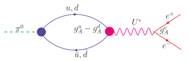
Figure 3: Loop diagram for $\pi^{0}\rightarrow e^{+}e^{-}$ process induced by the low mass exotic $U^{*}$ boson.

Further independent experiments at KLOE, NA48, WASAatCOSY, BES III and other facilities will be crucial for resolution of the problem. Also important is to get more precise data on the pion transition form factor in asymmetric as well in symmetric kinematics.

8 Acknowledgments

We are grateful to the Organizers for a nice meeting and kind invitation to present our results. Discussions on the subject of this work with C. Bloise, G. Collangelo, M.A. Ivanov, A. Kupcsh, E.A. Kuraev, M. P. Lombardo, E. Tomasi-Gustafsson were very helpful.

References

- [1] E. Abouzaid et al. Phys. Rev. D75 (2007) 012004.
- [2] S. Drell, Nuovo Cim. XI (1959) 693.
- [3] M. Berman and D.A. Geffen, Nuovo Cim. XVIII (1960) 1192.
- [4] L. Bergstrom, Z. Phys. C14 (1982) 129.
- [5] L. Bergstrom, E. Masso, L. Ametlier and A. Ramon, Phys. Lett. B126 (1983) 117.
- [6] G. D’Ambrosio and D. Espriu, Phys. Lett. B175, 237 (1986).
- [7] M. J. Savage, M. E. Luke, and M. B. Wise, Phys. Lett. B291, 481 (1992), hep-ph/9207233.
- [8] L. Ametller, A. Bramon, and E. Masso, Phys. Rev. D48, 3388 (1993), hep-ph/9302304.
- [9] G. V. Efimov, M. A. Ivanov, R. K. Muradov, and M. M. Solomonovich, JETP Lett. 34, 221 (1981).
- [10] A. E. Dorokhov and M. A. Ivanov, Phys. Rev. D75 (2007) 114007.
- [11] H. J. Behrend et al. [CELLO Collaboration], Z. Phys. C 49 (1991) 401.
- [12] CLEO, J. Gronberg et al., Phys. Rev. D57 (1998) 33.
- [13] A. E. Dorokhov, A. E. Radzhabov and M. K. Volkov, Eur. Phys. J. A 21 (2004) 155 [arXiv:hep-ph/0311359].
- [14] G. P. Lepage and S. J. Brodsky, Phys. Rev. D 22 (1980) 2157.
- [15] M. Berlowski et al., Phys. Rev. D 77 (2008) 032004.
- [16] R. Abegg et al., Phys. Rev. D 50 (1994) 92.
- [17] A. E. Dorokhov, E. A. Kuraev, Yu. M. Bystritskiy and M. Secansky, arXiv:0801.2028 [hep-ph].
- [18] L. Bergstrom, Z. Phys. C 20 (1983) 135.
- [19] A. E. Dorokhov and M. A. Ivanov, arXiv:0803.4493 [hep-ph].
- [20] C. Boehm and P. Fayet, Nucl. Phys. B 683 (2004) 219 [arXiv:hep-ph/0305261].
- [21] G. Weidenspointner et al., arXiv:astro-ph/0601673.
- [22] Y. Kahn, M. Schmitt, T. Tait, arXiv:0712.0007 [hep-ph].
- [23] P. Fayet, Phys. Rev. D75 115017 (2007).