On fine properties of mixtures with respect to
concentration of measure and Sobolev type inequalities

Abstract

Mixtures are convex combinations of laws. Despite this simple definition, a mixture can be far more subtle than its mixed components. For instance, mixing Gaussian laws may produce a potential with multiple deep wells. We study in the present work fine properties of mixtures with respect to concentration of measure and Sobolev type functional inequalities. We provide sharp Laplace bounds for Lipschitz functions in the case of generic mixtures, involving a transportation cost diameter of the mixed family. Additionally, our analysis of Sobolev type inequalities for two-component mixtures reveals natural relations with some kind of band isoperimetry and support constrained interpolation via mass transportation. We show that the Poincaré constant of a two-component mixture may remain bounded as the mixture proportion goes to $0$ or $1$ while the logarithmic Sobolev constant may surprisingly blow up. This counter-intuitive result is not reducible to support disconnections, and appears as a reminiscence of the variance-entropy comparison on the two-point space. As far as mixtures are concerned, the logarithmic Sobolev inequality is less stable than the Poincaré inequality and the sub-Gaussian concentration for Lipschitz functions. We illustrate our results on a gallery of concrete two-component mixtures. This work leads to many open questions.

Keywords. Mixtures of distributions; finite Gaussian mixtures; concentration of measure; Gaussian bounds; tails probabilities; deviation inequalities; functional inequalities; Poincaré inequalities; Gross logarithmic Sobolev inequalities; band isoperimetry; transportation of measure; mass transportation; transportation cost distances; Mallows or Wasserstein distance.

AMS-MSC. 60E15; 49Q20; 46E35; 62E99

1 Introduction

Mixtures of distributions are ubiquitous in Stochastic Analysis, Modelling, Simulation, and Statistics, see for instance the monographs [16, 18, 40, 39, 50]. Recall that a mixture of distributions is nothing else but a convex combination of these distributions. For instance, if $\mu_{0}$ and $\mu_{1}$ are two laws on the same space, and if $p\in[0,1]$ and $q=1-p$, then the law $p\mu_{1}+q\mu_{0}$ is a “two-component mixture”. More generally, a finite mixture takes the form $p_{1}\mu_{1}+\cdots+p_{n}\mu_{n}$ where $\mu_{1},\ldots,\mu_{n}$ are probability measures on a common measurable space and $p_{1}\delta_{1}+\cdots+p_{n}\delta_{n}$ is a finite discrete probability measure. A widely used example is given by finite mixtures of Gaussians for which $\mu_{i}=\mathcal{N}(m_{i},\sigma_{i}^{2})$ for every $1\leqslant i\leqslant n$. In that case, for certain choices of $m_{1},\ldots,m_{n}$ and $\sigma_{1},\ldots,\sigma_{n}$, the mixture

$$p_{1}\mathcal{N}(m_{1},\sigma_{1}^{2})+\cdots+p_{n}\mathcal{N}(m_{n},\sigma_{n}^{2})$$

is multi-modal and its log-density is a multiple wells potential. For instance, each component $\mu_{i}$ may correspond typically in Statistics to a sub-population, in Information Theory to a channel, and in Statistical Physics to an equilibrium. Another very natural example is given by the invariant measures of finite Markov chains, which are mixtures of the invariant measures uniquely associated to each recurrent class of the chain. A more subtle example is the local field of the Sherrington-Kirkpatrick model of spin glasses which gives rise to a mixture of two univariate Gaussians with equal variances, see for instance [13].

At this point, it is enlightening to introduce a bit more abstract point of view. Let $\nu$ be a probability measure on some measurable space $\Theta$ and $(\mu_{\theta})_{\theta\in\Theta}$ be a collection of probability measures on some common fixed measurable space $\mathcal{X}$, such that the map $\theta\mapsto\mathbf{E}_{\mu_{\theta}}f$ is measurable for any fixed bounded continuous $f:\mathcal{X}\to\mathbb{R}$. The mixture $\mathcal{M}(\nu,\mu_{\theta\in\Theta})$ is the law on $\mathcal{X}$ defined for any bounded measurable $f:\mathcal{X}\to\mathbb{R}$ by

$$\mathbf{E}_{\mathcal{M}(\nu,\mu_{\theta\in\Theta})}{f}=\int_{\Theta}\!\int_{\mathcal{X}}\!f(x)\,d\mu_{\theta}(x)\,d\nu(\theta)=\mathbf{E}_{\nu}(\theta\mapsto\mathbf{E}_{\mu_{\theta}}f).$$

Here $\nu$ is the mixing law whereas $(\mu_{\theta})_{\theta\in\Theta}$ are the mixed laws or the mixture components or even the mixed family. With these new notations, and for the finite mixture example mentioned earlier we have $\Theta=\{1,\ldots,n\}$ and $\nu=p_{1}\delta_{1}+\cdots+p_{n}\delta_{n}$ and

$$\mathcal{M}(\nu,(\mu_{\theta})_{\theta\in\Theta})=\mathcal{M}(p_{1}\delta_{1}+\cdots+p_{n}\delta_{n},\{\mu_{1},\ldots,\mu_{n}\})=p_{1}\mu_{1}+\cdots+p_{n}\mu_{n}.$$

The mixture $\mathcal{M}(\nu,\mu_{\theta\in\Theta})$ can be seen as a sort of general convex combination in the convex set of probability measures on $\mathcal{X}$. It appears for certain class of $\nu$ as a particular Choquet’s Integral, see [43] and [17]. On the other hand, the case where the mixture components are product measures is also related to exchangeability and De Finetti’s Theorem, see for instance [7]. In terms of random variables, if $(X,Y)$ is a couple of random variables then the law $\mathcal{L}(X)$ of $X$ is a mixture of the family of conditional laws $\mathcal{L}(X|Y=y)$ with the mixing law $\mathcal{L}(Y)$. By this way, mixing appears as the dual of the so-called disintegration of measure. Here and in the whole sequel, the term “mixing” refers to the mixture of distributions as defined above and has a priori nothing to do with weak dependence.

Our first aim is to investigate the fine behavior of concentration of measure for mixtures, for instance for a two-component mixture $p\mu_{1}+q\mu_{0}$ as $\min(p,q)$ goes to $0$. It is well known that Poincaré and (Gross) logarithmic Sobolev functional inequalities are powerful tools in order to obtain concentration of measure. Also, our second aim is to investigate the fine behavior of these functional inequalities for mixtures, and in particular for two-component mixtures. Our work reveals striking unexpected phenomena. In particular, our results suggest that the logarithmic Sobolev inequality, which implies sub-Gaussian concentration, is very sensitive to mixing, in contrast with the sub-Gaussian concentration itself which is far more stable. As in [20] and [3], our work is connected to the more general problem of the behavior of optimal constants for sequences of probability measures.

Let us start with the notion of concentration of measure for Lipschitz functions. We denote by ${{\left\|\cdot\right\|}}_{2}$ the Euclidean norm of $\mathbb{R}^{d}$. A function $f:\mathbb{R}^{d}\to\mathbb{R}$ is Lipschitz when

$${\|f\|_{\mathrm{Lip}}}=\sup_{x\neq y}\frac{|f(x)-f(y)|}{{{\left\|x-y\right\|}}_{2}}<\infty.$$

Let $\mu$ be a law on $\mathbb{R}^{d}$ such that $\mathbf{E}_{\mu}|f|<\infty$ for every Lipschitz function $f$. This holds true for instance when $\mu$ has a finite first moment. We always make implicitly this assumption in the sequel. We define now the log-Laplace transform $\alpha_{\mu}:\mathbb{R}\to[0,\infty]$ of $\mu$ by

$$\alpha_{\mu}(\lambda)=\log\sup_{{\|f\|_{\mathrm{Lip}}}\leqslant 1}\mathbf{E}_{\mu}{{\left(e^{\lambda(f-\mathbf{E}_{\mu}{f})}\right)}}.$$ (1)

The Cramér-Chernov-Chebychev inequality gives, for every $r>0$,

$$\beta_{\mu}(r)=\sup_{{\|f\|_{\mathrm{Lip}}}\leqslant 1}\mu{{\left({{\left|f-\mathbf{E}_{\mu}f\right|}}\geqslant r\right)}}\leqslant 2\exp{{\left(-\sup_{\lambda>0}{{\left(r\lambda-\alpha_{\mu}(\lambda)\right)}}\right)}}$$ (2)

and the supremum in the right hand side is a Fenchel-Legendre transform of $\alpha_{\mu}$. Note that $\beta_{\mu}$ is a uniform upper bound on the tails probabilities of Lipschitz images of $\mu$. We are interested in the control of $\beta_{\mu}$ via $\alpha_{\mu}$ in the case where $\mu=\mathcal{M}(\nu,(\mu_{\theta})_{\theta\in\Theta})$, in terms of the mixing law $\nu$ and of the log-Laplace bounds $(\alpha_{\mu_{\theta}})_{\theta\in\Theta}$ for the mixed family.

We say that $\mu$ satisfies a sub-Gaussian concentration of measure for Lipschitz functions when there exists a constant $C\in(0,\infty)$ such that for every real number $\lambda$,

$$\alpha_{\mu}(\lambda)\leqslant\frac{1}{4}C\lambda^{2}.$$ (3)

The $\log$-Laplace-Lipschitz quadratic bound (3) implies via (2) that for every $r>0$,

$$\beta_{\mu}(r)\leqslant 2\exp{{\left(-\frac{r^{2}}{C}\right)}}.$$ (4)

Actually, it was shown (see [15] and [9]) that up to constants, (3) and (4) are equivalent, and are also equivalent to the existence of a constant $\varsigma\in(0,\infty)$ and $x_{0}\in\mathbb{R}^{d}$ such that

$$\int_{\mathbb{R}^{d}}\!e^{\varsigma|x-x_{0}|^{2}}\,\mu(dx)<\infty.$$ (5)

Linear or quadratic upper bounds for $\alpha_{\mu}$ may be deduced from functional inequalities such as Poincaré and (Gross) logarithmic Sobolev inequalities [23, 24]. We say that $\mu$ satisfies a Poincaré inequality of constant $C\in(0,\infty)$ when for every smooth $h:\mathbb{R}^{d}\to\mathbb{R}$,

$$\mathbf{Var}_{\mu}(h)\leqslant C\,\mathbf{E}(|\nabla h|^{2})$$ (6)

where $\mathbf{Var}_{\mu}(h)=\mathbf{E}_{\mu}(h^{2})-(\mathbf{E}_{\mu}h)^{2}$ is the variance of $h$ for $\mu$. The smallest possible constant $C$ is called the optimal Poincaré constant of $\mu$ and is denoted $C_{\textsc{PI}}(\mu)$ with the convention $\inf\emptyset=\infty$. Similarly, $\mu$ satisfies a (Gross) logarithmic Sobolev inequality of constant $C\in(0,\infty)$ when

$$\mathbf{Ent}_{\mu}(h^{2})\leqslant C\,\mathbf{E}(|\nabla h|^{2})$$ (7)

for every smooth function $f:\mathbb{R}^{d}\to\mathbb{R}$, where $\mathbf{Ent}_{\mu}(h^{2})=\mathbf{E}_{\mu}(h^{2}\log h^{2})-\mathbf{E}_{\mu}(h^{2})\log\mathbf{E}_{\mu}(h^{2})$ is the entropy or free energy of $h^{2}$ for $\mu$, with the convention $0\log(0)=0$. As for the Poincaré inequality, the smallest possible $C$ is the optimal logarithmic Sobolev constant of $\mu$ and is denoted $C_{\textsc{GI}}(\mu)$ with $\inf\emptyset=\infty$. Standard linearization arguments give that

$$\rho(K_{\mu})\leqslant C_{\textsc{PI}}(\mu)\leqslant\frac{1}{2}\,C_{\textsc{GI}}(\mu)$$ (8)

where $\rho(K_{\mu})$ stands for the spectral radius of the covariance matrix $K_{\mu}$ of $\mu$ defined by $(K_{\mu})_{i,j}=\mathbf{E}_{\mu}(x_{i}x_{j})-\mathbf{E}_{\mu}(x_{i})\mathbf{E}_{\mu}(x_{j})$ where $x_{i}$ and $x_{j}$ are the coordinate functions. More precisely, the first inequality in (8) follows from (6) by taking $h={{\left<\cdot,u\right>}}$ where $u$ runs over the unit sphere while the second inequality in (8) follows by considering the directional derivative of both sides of (7) at the constant function $1$.

A basic example is given by Gaussian laws for which equalities are achieved in (8). A wide class of laws satisfy Poincaré and logarithmic Sobolev inequalities. Beyond Gaussian laws, a criterion due to Bakry & Émery [2, 1] (see also [42], [46, 12], and [10, 11]) states that if $\mu$ has Lebesque density $e^{-V}$ on $\mathbb{R}^{d}$ such that $x\mapsto V(x)-\frac{1}{2\kappa}|x|^{2}$ is convex for some fixed real $\kappa>0$ then $C_{\textsc{PI}}(\mu)\leqslant\kappa$ and $C_{\textsc{GI}}(\mu)\leqslant 2\kappa$ with equality in both cases when $\mu$ is Gaussian. This log-concave criterion appears as a comparison with Gaussians. Note that in general, $C_{\textsc{GI}}(\mu)<\infty$ implies $C_{\textsc{PI}}(\mu)<\infty$ but the converse is false. For instance, the law with density proportional to $\exp(-|x|^{a})$ on $\mathbb{R}$ satisfies a Poincaré inequality iff $a\geqslant 1$ and a logarithmic Sobolev inequality iff $a\geqslant 2$, see e.g. [1, Chapter 6]. Note also that if $\mu$ has disconnected support, then necessarily $C_{\textsc{PI}}(\mu)=C_{\textsc{GI}}(\mu)=\infty$. To see it, consider a non constant $h$ which is constant on each connected component of the support of $\mu$. This is for instance the case for the two-component mixture $\mu=p\mu_{1}+q\mu_{0}=\mathcal{M}(p\delta_{1}+q\delta_{0},\{\mu_{0},\mu_{1}\})$ with $p\in(0,1)$ and $q=1-p$ where $\mu_{0}$ and $\mu_{1}$ have disjoint supports.

The logarithmic Sobolev inequality (7) implies a sub-Gaussian concentration of measure for Lipschitz images of $\mu$. Namely, using (7) with $h=\exp(\frac{1}{2}\lambda f)$ for a real number $\lambda$ and a smooth Lipschitz function $f:\mathbb{R}^{d}\to\mathbb{R}$ gives via Rademacher’s Theorem and a standard argument attributed to Herbst [34, Chapter 5] that for any reals $\lambda$ and $r>0$

$$\alpha_{\mu}(\lambda)\leqslant\frac{1}{4}C_{\textsc{GI}}(\mu)\lambda^{2}\quad\text{and}\quad\beta_{\mu}(r)\leqslant 2\exp{{\left(-\frac{r^{2}}{C_{\textsc{GI}}(\mu)}\right)}}.$$ (9)

The same method yields from (6) a sub-exponential upper bound for $\beta_{\mu}$ of the form $c_{1}\exp(-c_{2}r)$ for some constants $c_{1},c_{2}>0$, see for instance [22] and [33, Section 2.5].

Both Poincaré and logarithmic Sobolev inequalities are invariant by the action of the translation group and the orthogonal group. More generally, let us denote by $f\cdot\mu$ the image measure of $\mu$ by the map $f$. Both (6) and (7) are stable by Lipschitz maps in the sense that $C_{\textsc{PI}}(f\cdot\mu)\leqslant{{\left\|f\right\|}}^{2}_{\textsc{Lip}}C_{\textsc{PI}}(\mu)$ and $C_{\textsc{GI}}(f\cdot\mu)\leqslant{{\left\|f\right\|}}^{2}_{\textsc{Lip}}C_{\textsc{GI}}(\mu)$. On the real line, $C_{\textsc{PI}}$ and $C_{\textsc{GI}}$ can be controlled via “simple” variational bounds such as (18). Both (6) and (7) are also stable by bounded perturbations on the log-density of $\mu$, see [27], [25], and [3] for further details. In view of sub-exponential or sub-Gaussian concentration bounds, the main advantage of (6) and (7) over a direct approach based on $\alpha_{\mu}$ or $\beta_{\mu}$ lies in the stability by tensor products of (6) and (7), see e.g. [1, Chapters 1 and 3], [9], and [21].

The case of mixtures. The integral criterion (5) shows that if the components of a mixture satisfies uniformly a sub-Gaussian concentration of measure for Lipschitz functions, and if the mixing law has compact support, then the mixture also satisfies a sub-Gaussian concentration of measure for Lipschitz functions. Such bounds appear for instance in [6]. However, this observation does not give any fine quantitative estimate on the dependency over the weights for a finite mixture. Regarding Poincaré and logarithmic Sobolev inequalities, it is clear that a finite mixture of Gaussians will satisfies such inequalities since its log-density is a bounded perturbation of a uniformly concave function. Here again, this does not give any fine control on the constants.

An upper bound for the Poincaré constant of univariate finite Gaussian mixture was provided by Johnson [29, Theorem 1.1 and Section 2]. Unfortunately, this upper bound blows up when the minimum weight of the mixing law goes to $0$. A more general upper bound for finite mixtures of overlapping densities was obtained by Madras and Randall [35, Theorem 1.2 and Section 5]. Here again, the bound blows up when the minimum weight of the mixing law goes to $0$. Some aspects of Poisson mixtures are considered by Kontoyannis and Madiman [30, 31] in connection with compound Poisson processes and discrete modified logarithmic Sobolev inequalities.

Outline of the article. Recall that the aim of the present work is to study fine properties of mixture of law with respect to concentration of measure and Sobolev type functional inequalities. The analysis of various elementary examples shows actually that such a general objective is very ambitious. Also, we decided to focus in the present work on more tractable situations. Section 2 provides Laplace bounds for Lipschitz functions in the case of generic mixtures. These upper bounds on $\alpha_{\mu}$ (and thus $\beta_{\mu}$) for a mixture $\mu$ involve the $W_{1}$-diameter (see Section 2 for a precise definition) of the mixed family. Section 3 is devoted to upper bounds on $\alpha_{\mu}$ for two-component mixtures $\mu=\mu_{p}=p\mu_{1}+q\mu_{0}$. Our result is mainly based on a Laplace-Lipschitz counterpart of the optimal logarithmic Sobolev inequality for asymmetric Bernoulli measures. In particular, we show that if $\mu_{0}$ and $\mu_{1}$ satisfy a sub-Gaussian concentration for Lipschitz functions, then it is also the case for the mixture $\mu_{p}$, with a quite satisfactory and intuitive behavior as $\min(p,q)$ goes to $0$. In Section 4, we study Poincaré and logarithmic Sobolev inequalities for two components mixtures. A decomposition of variance and entropy allows to reduce the problem to the Poincaré and logarithmic Sobolev inequalities for each component, to discrete inequalities for the Bernoulli mixing law $p\delta_{1}+q\delta_{0}$, and to the control of a mean-difference term. This last term can be controlled in turn by using some support-constrained transportation, leading to very interesting open questions in dimension $>1$. The Poincaré constant of the two-component mixture can remain bounded as $\min(p,q)$ goes to $0$, while the logarithmic Sobolev constant may surprisingly blow up at speed $-\log(\min(p,q))$. This counter-intuitive result shows that as far as mixture of laws are concerned, the logarithmic Sobolev inequality does not behave like the sub-Gaussian concentration for Lipschitz functions. We also illustrate our results on a gallery of concrete two-component mixtures. In particular, we show that the blow up of the logarithmic Sobolev constant as $\min(p,q)$ goes to $0$ is not necessarily related to support problems.

Open problems. The study of Poincaré and logarithmic Sobolev inequalities for multivariate or non-finite mixtures is an interesting open problem, for which we give some clues at the end of Section 4 in terms of support-constrained transportation interpolation. There is maybe a link with the decomposition approach used in [28] for Markov chains. One can also explore the tensor products of mixtures, which are again mixtures. Another interesting problem is the development of a direct approach for transportation cost and measure-capacities inequalities (see [5]) for mixtures, even in the finite univariate case.

2 General Laplace bounds for Lipschitz functions

Intuitively, the concentration of measure of a finite mixture may be controlled by the worst concentration of the components and some sort of diameter of the mixed family. We shall confirm, extend, and illustrate this intuition for a non necessarily finite mixture. The notion of diameter that we shall use is related to coupling and transportation cost. Recall that for every $k\geqslant 1$, the Wasserstein (or transportation cost) distance of order $k$ between two laws $\mu_{1}$ and $\mu_{2}$ on $\mathbb{R}^{d}$ is defined by (see e.g. [51, 52] and [44, 47])

$$W_{k}(\mu_{1},\mu_{2})=\inf_{\pi}{{\left(\int_{\mathbb{R}^{d}\times\mathbb{R}^{d}}\!|x-y|^{k}\,d\pi(x,y)\right)}}^{k^{-1}}$$ (10)

where $\pi$ runs over the set of laws on $\mathbb{R}^{d}\times\mathbb{R}^{d}$ with marginals $\mu_{1}$ and $\mu_{2}$. The $W_{k}$-convergence is equivalent to the weak convergence together with the convergence of moments up to order $k$. In dimension $d=1$, we have, by denoting $F_{1}$ and $F_{2}$ the cumulative distribution functions of $\mu_{1}$ and $\mu_{2}$, with generalized inverses $F_{1}^{-1}$ and $F_{2}^{-1}$, for every $k\geqslant 1$,

$$W_{k}(\mu_{1},\mu_{2})^{k}=\!\int_{0}^{1}\!{{\left|F_{1}^{-1}(x)-F_{2}^{-1}(x)\right|}}^{k}\,dx\ \ \text{and}\ \ W_{1}(\mu_{1},\mu_{2})=\!\int_{\mathbb{R}}\!{{\left|F_{1}(x)-F_{2}(x)\right|}}\,dx$$ (11)

where the last expression of $W_{1}$ follows from the Kantorovich-Rubinstein dual formulation

$$W_{1}(\mu_{1},\mu_{2})=\sup_{{\|f\|_{\mathrm{Lip}}}\leqslant 1}{{\left(\int_{\mathbb{R}^{d}}\!f\,d\mu_{1}-\int_{\mathbb{R}^{d}}\!f\,d\mu_{2}\right)}}.$$ (12)

Note that if $\mu_{1}$ does not give mass to points then $\mu_{2}=(F_{2}^{-1}\circ F_{1})\cdot\mu_{1}$. The transportation cost distances lead to the so called transportation cost inequalities, popularized by Marton [36, 37], Talagrand [49], and Bobkov & Götze [8]. See for instance the books [34, 51, 52] for a review. The link with concentration of measure was recently deeply explored by Gozlan, see e.g. [21]. We will not use this interesting line of research in the present paper.

Theorem 2.1 (General Laplace-Lipschitz bound via diameter).

Let $\mu=\mathcal{M}(\nu,{(\mu_{\theta})}_{\theta\in\Theta})$ be a general mixture. If this mixture satisfies the uniform bounds

$$\overline{\alpha}=\sup_{\theta\in\Theta}\alpha_{\theta}<\infty\quad\text{and}\quad\overline{W}=\sup_{\theta,\theta^{\prime}\in\Theta}W_{1}(\mu_{\theta},\mu_{\theta^{\prime}})<\infty$$

then for every $\lambda>0$ we have

$$\alpha_{\mu}(\lambda)\leqslant\overline{\alpha}(\lambda)+\frac{1}{8}\min{{\left(8\overline{W}\lambda,\overline{W}^{2}\lambda^{2}\right)}}.$$

Proof of Theorem 2.1.

The key point is that if ${\|f\|_{\mathrm{Lip}}}\leqslant 1$ then for every $\lambda>0$,

$$\frac{\mathbf{E}_{\mu}{{\left(e^{\lambda f}\right)}}}{e^{\lambda\mathbf{E}_{\mu}f}}=e^{-\lambda\mathbf{E}_{\mu}f}\int_{\Theta}\!\mathbf{E}_{\mu_{\theta}}{{\left(e^{\lambda f}\right)}}\,\nu(d\theta)\leqslant\int_{\Theta}\!e^{\alpha_{\theta}(\lambda)+\lambda(\mathbf{E}_{\mu_{\theta}}f-\mathbf{E}_{\mu}f)}\,\nu(d\theta).$$ (13)

As a consequence, we get

$$\alpha_{\mu}(\lambda)\leqslant\overline{\alpha}(\lambda)+\sup_{{\|f\|_{\mathrm{Lip}}}\leqslant 1}\log\int_{\Theta}\!e^{\lambda(\mathbf{E}_{\mu_{\theta}}f-\mathbf{E}_{\mu}f)}\,\nu(d\theta).$$ (14)

Thanks to the relation (12), we obtain

$$\mathbf{E}_{\mu_{\theta}}f-\mathbf{E}_{\mu}f =\int_{\Theta}\!{{\left(\mathbf{E}_{\mu_{\theta}}f-\mathbf{E}_{\mu_{\theta^{\prime}}}f\right)}}\,\nu(d\theta^{\prime})$$

$$\leqslant\int_{\Theta}\!W_{1}(\mu_{\theta},\mu_{\theta^{\prime}})\,\nu(d\theta^{\prime})\leqslant\overline{W}.$$

This shows that the second term in the right hand side of (14) is bounded by $\overline{W}\lambda$. Alternatively, one can use the Hoeffding bound [26] which says that if $X$ is a centered bounded random variable with oscillation $c=\sup X-\inf X$ then

$$\mathbf{E}{{\left(e^{\lambda X}\right)}}\leqslant e^{\frac{1}{8}\lambda^{2}c^{2}}.$$

The desired bound in terms of $\overline{W}^{2}\lambda^{2}$ follows by taking $X=\mathbf{E}_{\mu_{Y}}f-\mathbf{E}_{\mu}f$ where $Y\sim\nu$ and noticing that $c\leqslant\sup_{\theta,\theta^{\prime}}{{\left(\mathbf{E}_{\mu_{\theta}}f-\mathbf{E}_{\mu_{\theta^{\prime}}}f\right)}}=\overline{W}$. ∎

Example 2.2 (Finite mixtures).

For a finite mixture $\mu=p_{1}\mu_{1}+\cdots+p_{n}\mu_{n}=\mathcal{M}(\nu,(\mu_{i})_{1\leqslant i\leqslant n})$ where $\nu=p_{1}\delta_{1}+\cdots+p_{n}\delta_{n}$, the mixing measure $\nu$ is supported by a finite set. In that case, Theorem 2.1 gives an immediate Laplace bound, involving the worst bound for the mixture components $(\mu_{i})_{1\leqslant i\leqslant n}$ (this cannot be improved in general). However, in Section 3, we provide sharper bounds by improving the dependency over $\nu$ in the case where $n=2$.

Example 2.3 (Bounded mixtures of multivariate Gaussians).

Here $\mu_{\theta}=\mathcal{N}(m(\theta),\Gamma(\theta))$ where $m:\Theta\to\mathbb{R}^{d}$ and $\Gamma:\mathbb{R}^{d}\to\mathcal{S}^{+}_{d}$ are two measurable bounded functions and $\mathcal{S}^{+}_{d}$ is the cone of symmetric nonnegative $d\times d$ matrices. Note that $\Gamma(\theta)$ is allowed to be singular i.e. not of full rank. The spectrum of $\Gamma(\theta)$ is real and non-negative. If $\lambda_{1}(\theta)\geqslant\cdots\geqslant\lambda_{d}(\theta)$ are the eigenvalues of $\Gamma(\theta)$, we define $\rho=\sup_{\theta\in\Theta}\lambda_{1}(\theta)=\sup_{\theta\in\Theta}{{\left\|\Gamma(\theta)\right\|}}_{2\to 2}$. Now fix some mixing law $\nu$ on $\Theta$ and consider the mixture $\mu=\mathcal{M}(\nu,{(\mu_{\theta})}_{\theta\in\Theta})$. Then for every $\lambda>0$,

$$\alpha_{\mu}(\lambda)\leqslant\frac{\rho}{2}\lambda^{2}+\frac{1}{8}\min(8\overline{W}\lambda,\overline{W}^{2}\lambda^{2}).$$

One can deduce an upper bound for $\overline{W}$ from the following lemma.

Lemma 2.4 ($W_{1}$-distance of two multivariate Gaussian laws).

Let $\mu_{0}=\mathcal{N}(m(0),\Gamma(0))$ and $\mu_{1}=\mathcal{N}(m(1),\Gamma(1))$ be two Gaussian laws on $\mathbb{R}^{d}$. For $\theta\in\{0,1\}$, we denote by

$$\lambda_{1}(\theta)\geqslant\cdots\geqslant\lambda_{d}(\theta)$$

the ordered spectrum of $\Gamma(\theta)$ and by ${(v_{i}{(\theta)})}_{1\leqslant i\leqslant d}$ an associated orthonormal basis of eigenvectors. Assume, without loss of generality, that $v_{i}{(0)}\cdot v_{i}{(1)}\geqslant 0$ for every $1\leqslant i\leqslant d$ where “$\cdot$” stands for the Euclidean scalar product of $\mathbb{R}^{d}$. Then $W_{1}(\mu_{0},\mu_{1})$ is bounded above by

$${{\left|m(1)-m(0)\right|}}+\sqrt{\sum_{i=1}^{d}{{\left\{{{\left(\sqrt{\lambda_{i}{(1)}}-\sqrt{\lambda_{i}{(0)}}\right)}}^{2}+2\sqrt{\lambda_{i}{(1)}\lambda_{i}{(0)}}{{\left(1-v_{i}{(1)}\cdot v_{i}{(0)}\right)}}\right\}}}}.$$

The reader may find in [48, Theorem 3.2] a formula in the same spirit for $W_{2}(\mu_{0},\mu_{1})$.

Proof of Lemma 2.4.

The triangle inequality for the $W_{1}$ distance gives

$$W_{1}(\mu_{0},\mu_{1}) \leqslant W_{1}(\mu_{0},\mathcal{N}(m(1),\Gamma(0)))+W_{1}(\mathcal{N}(m(1),\Gamma(0)),\mu_{1})$$

$$\leqslant{{\left|m(1)-m(0)\right|}}+W_{1}(\mathcal{N}(0,\Gamma(0)),\mathcal{N}(0,\Gamma(1))).$$

Now, if ${(Y_{i})}_{1\leqslant i\leqslant d}$ are i.i.d. real random variables of law $\mathcal{N}(0,1)$ then the law of

$$X_{\theta}=\sum_{i=1}^{d}Y_{i}\sqrt{\lambda_{i}{(\theta)}}v_{i}{(\theta)}$$

is $\mathcal{N}(0,\Gamma(\theta))$ for $\theta\in\{0,1\}$. Moreover, from (10) and Jensen’s inequality, we get

$$W_{1}(\mathcal{N}(0,\Gamma(0)),\mathcal{N}(0,\Gamma(1)))^{2}\leqslant{{\left(\mathbb{E}{{\left|X_{1}-X_{0}\right|}}\right)}}^{2}\leqslant\mathbb{E}({{\left|X_{1}-X_{0}\right|}}^{2}).$$

At this step, we note that

$${{\left|X_{1}-X_{0}\right|}}^{2}= \sum_{i=1}^{d}Y_{i}^{2}{{\left|\sqrt{\lambda_{i}(1)}v_{i}(1)-\sqrt{\lambda_{i}(0)}v_{i}(0)\right|}}^{2}$$

$$+2\sum_{i<j}Y_{i}Y_{j}{{\left(\sqrt{\lambda_{i}(1)}v_{i}(1)-\sqrt{\lambda_{i}(0)}v_{i}(0)\right)}}\cdot{{\left(\sqrt{\lambda_{i}(1)}v_{i}(1)-\sqrt{\lambda_{i}(0)}v_{i}(0)\right)}}.$$

Since ${(Y_{i})}$ are i.i.d. $\mathcal{N}(0,1)$ and ${(v_{i}(\theta))}_{1\leqslant i\leqslant d}$ is orthonormal for $\theta\in\{0,1\}$, one has

$$\mathbb{E}({{\left|X_{1}-X_{0}\right|}}^{2}) =\sum_{i=1}^{d}{{\left|\sqrt{\lambda_{i}(1)}v_{i}(1)-\sqrt{\lambda_{i}(0)}v_{i}(0)\right|}}^{2}$$

$$=\sum_{i=1}^{d}{{\left\{{{\left(\sqrt{\lambda_{i}{(1)}}-\sqrt{\lambda_{i}{(0)}}\right)}}^{2}+2\sqrt{\lambda_{i}{(1)}\lambda_{i}{(0)}}{{\left(1-v_{i}{(1)}\cdot v_{i}{(0)}\right)}}\right\}}}.$$

∎

Of course the assumptions of Theorem 2.1 may be relaxed. Instead of trying to deal with generic abstract results, let us provide some highlighting examples.

Example 2.5 (Gaussian mixture of translated Gaussians).

Here $\Theta=\mathbb{R}$ and $\mu_{\theta}=\mathcal{N}(\theta,\sigma^{2})$ for some fixed $\sigma>0$, and the mixing law is also Gaussian $\nu=\mathcal{N}(0,\tau^{2})$ for some fixed $\tau>0$. In this case, $\overline{\alpha}(\lambda)=\frac{1}{2}\sigma^{2}\lambda^{2}$ but $\overline{W}$ is infinite since

$$W_{1}(\mu_{\theta},\mu_{\theta^{\prime}})={{\left|\theta-\theta^{\prime}\right|}}.$$

In particular, Theorem 2.1 is useless. Nevertheless, the function

$$\theta\mapsto g(\theta)=\mathbf{E}_{\mu_{\theta}}f-\mathbf{E}_{\mu}f$$

is Lipschitz since

$${{\left|g(\theta)-g(\theta^{\prime})\right|}}\leqslant\mathbf{E}{{\left({{\left|f(X+\theta)-f(X+\theta^{\prime})\right|}}\right)}}\leqslant{{\left|\theta-\theta^{\prime}\right|}}$$

where $X\sim\mathcal{N}(0,1)$. As a consequence, we get

$$\sup_{{\|f\|_{\mathrm{Lip}}}\leqslant 1}\log\int_{\Theta}\!e^{\lambda(\mathbf{E}_{\mu_{\theta}}f-\mathbf{E}_{\mu}f)}\,\nu(d\theta)\leqslant\frac{\tau^{2}\lambda^{2}}{2},$$

and for any $\lambda>0$

$$\alpha_{\mu}(\lambda)\leqslant\frac{\sigma^{2}+\tau^{2}}{2}\lambda^{2}.$$

The same argument may be used more generally for “position” mixtures. For instance if $\eta$ is some fixed probability measure on $\mathbb{R}^{d}$ and $\mu_{\theta}=\eta*\delta_{\theta}$ for $\theta\in\mathbb{R}^{d}$ then $\forall\lambda>0$,

$$\alpha_{\mu}(\lambda)\leqslant\alpha_{\eta}(\lambda)+\alpha_{\mu}(\lambda).$$

In this particular case, $\mu=\nu*\eta$ and the bound above follows also by tensorization!

Example 2.6 (Mixture of scaled Gaussians: from exponential to Gaussian tails).

Here we take $\Theta=[0,\infty)$ and $\mu_{\theta}=\mathcal{N}(0,\theta^{2})$ with a mixing measure $\nu$ of density

$$\theta\mapsto\frac{\gamma}{\Gamma\!{{\left(\gamma^{-1}\right)}}}\exp{{\left(-\theta^{\gamma}\right)}}\mathds{1}_{[0,\infty)}(\theta)$$

where $\gamma\geqslant 2$ is some fixed real number. Note that $\nu$ has a non-compact support and that $\mu$ does not satisfy the integral criterion (5). This means that $\mu$ cannot have sub-Gaussian tails. Note also that both $\overline{\alpha}(\lambda)$ and $\overline{W}$ are infinite since

$$\alpha_{\theta}(\lambda)=\frac{\theta^{2}\lambda^{2}}{2}\quad\text{and}\quad W_{1}(\mu_{\theta},\mu_{\theta^{\prime}})=\sqrt{\frac{2}{\pi}}\,{{\left|\theta-\theta^{\prime}\right|}}$$

where we used (11) for $W_{1}$. Starting from (13), one has by Cauchy-Schwarz’s inequality

$${{\left(\frac{\mathbf{E}_{\mu}{{\left(e^{\lambda f}\right)}}}{e^{\lambda\mathbf{E}_{\mu}f}}\right)}}^{2}\leqslant\int_{\Theta}\!e^{\theta^{2}\lambda^{2}}\,\nu(d\theta)\int_{\Theta}\!e^{2\lambda(\mathbf{E}_{\mu_{\theta}}f-\mathbf{E}_{\mu}f)}\,\nu(d\theta).$$ (15)

Note that $\nu$ satisfies condition (5) and $\alpha_{\nu}(\lambda)\leqslant C\lambda^{2}$ for some real constant $C>0$. Here and in the sequel, the constant $C$ may vary from line to line and may be chosen independent of $\gamma$. On the other hand, the centered function $g(\theta)=\mathbf{E}_{\mu_{\theta}}f-\mathbf{E}_{\mu}f$ is 1-Lipschitz since

$${{\left|g(\theta)-g(\theta^{\prime})\right|}}={{\left|\mathbf{E}f(\theta X)-\mathbf{E}f(\theta^{\prime}X)\right|}}\leqslant{{\left|\theta-\theta^{\prime}\right|}}\mathbf{E}({{\left|X\right|}})$$

where $X\sim\mathcal{N}(0,1)$. Also, for the second term in the right hand side of (15) we have

$$\int_{\Theta}\!e^{2\lambda(\mathbf{E}_{\mu_{\theta}}f-\mathbf{E}_{\mu}f)}\,\nu(d\theta)\leqslant e^{\alpha_{\nu}(2\lambda)}\leqslant e^{4C\lambda^{2}}.$$

If $\gamma=2$ then $\alpha_{\mu}(\lambda)\leqslant 2C\lambda^{2}-\frac{1}{4}\log(1-\lambda^{2})\leqslant 2C-\frac{1}{4}\log(1-\lambda)$ if $\lambda<1$, which gives, after some computations, the deviation bound, for some other constants $C^{\prime}>0$ and $C^{\prime\prime}>0$,

$$\mu(F-\mathbf{E}_{\mu}f\geqslant r)\leqslant C^{\prime}e^{-C^{\prime\prime}r}.$$

Assume in contrast that $\gamma>2$. Since $\theta^{2}\lambda^{2}\leqslant\gamma^{-1}\theta^{\gamma}+C_{0}\lambda^{\frac{2\gamma}{\gamma-2}}$ for some constant $C_{0}>0$ which may depend on $\gamma$ but not on $\lambda$ and $\theta$, we get, for some constants $C_{1}>0$ and $C_{2}>0$,

$$\int_{0}^{\infty}\!\exp{{\left(\theta^{2}\lambda^{2}\right)}}\,\nu(d\theta)\leqslant C_{1}\exp{{\left(C_{2}\lambda^{\frac{2\gamma}{\gamma-2}}\right)}}.$$

This gives $\alpha_{\mu}(\lambda)\leqslant{}C_{3}\lambda^{\frac{2\gamma}{\gamma-2}}+C_{4}$ for some constants $C_{3}>0$ and $C_{4}>0$, which yields a deviation bound of the form (for some constants $C_{5}>0$ and $C_{6}>0$)

$$\mu(f-\mathbf{E}_{\mu}f\geqslant r)\leqslant C_{5}\exp{{\left(-C_{6}r^{2-\frac{4}{\gamma+2}}\right)}}.$$

Note that $\nu$ goes to the uniform law on $[0,1]$ as $\gamma\to\infty$ and the Gaussian tail reappears.

3 Concentration bounds for two-component mixtures

In this section, we investigate the special case where the mixing measure $\nu$ is the Bernoulli measure $\mathcal{B}(p)=p\delta_{1}+q\delta_{0}$ where $q=1-p$. We are interested in the study of the sharp dependence of the concentration bounds on $p$, especially when $p$ is close to $0$ or $1$.

Theorem 3.1 (Two-component mixture).

Let $\mu_{0}$ and $\mu_{1}$ be two probability measures on $\mathcal{X}$ and $\mu=p\mu_{1}+q\mu_{0}$ with $p\in[0,1]$ and $q=1-p$. Define $x_{p}=\max(p,q)/(2c_{p})$ where

$$c_{p}=\frac{q-p}{4(\log(q)-\log(p))}$$

with the continuity conventions $c_{1/2}=1/8$ and $c_{0}=c_{1}=0$. Then for any $\lambda>0$,

$$\alpha_{\mu}(\lambda)\leqslant\max(\alpha_{\mu_{0}},\alpha_{\mu_{1}})(\lambda)+\begin{cases}\displaystyle{c_{p}\lambda^{2}W_{1}(\mu_{0},\mu_{1})^{2}}&\text{if $\lambda W_{1}(\mu_{0},\mu_{1})\leqslant x_{p}$}\\ \\ \displaystyle{\max(p,q){{\left(\lambda W_{1}(\mu_{0},\mu_{1})-\frac{1}{2}x_{p}\right)}}}&\text{otherwise}.\end{cases}$$

Note that if $\min(p,q)\to 0$, then $c_{p}\sim-(4\log(p))^{-1}\to 0$ and $x_{p}\to\infty$, and we thus recover an upper bound of the form $\alpha_{\mu}\leqslant\max(\alpha_{\mu_{1}},\alpha_{\mu_{2}})$ as $\min(p,q)\to 0$, which is satisfactory. The two different upper bounds given by Theorem 3.1 provide two different upper bounds for the concentration of measure of the mixture $\mu$, illustrated by the following Corollary (the proof of the Corollary is immediate and is left to the reader).

Corollary 3.2 (Two-component mixtures with sub-Gaussian tails).

Let $\mu_{0}$ and $\mu_{1}$ be two probability measures on $\mathcal{X}$ and $\mu=p\mu_{1}+q\mu_{0}$ for some $p\in[0,1]$ with $q=1-p$. If there exists a real constant $C>0$ such that for any $\lambda>0$

$$\max(\alpha_{\mu_{0}},\alpha_{\mu_{1}})(\lambda)\leqslant\frac{1}{2}C\lambda^{2}$$

then for every $r\geqslant 0$, with $\overline{W}=W_{1}(\mu_{0},\mu_{1})$,

$$\beta_{\mu}(r)\leqslant 2\begin{cases}\displaystyle{\exp{{\left(-\frac{r^{2}}{2C+4c_{p}\overline{W}^{2}}\right)}}}&\text{if $r\leqslant\max(p,q){{\left(\frac{C}{2c_{p}\overline{W}}+\overline{W}\right)}}$},\\ &\\ \displaystyle{\exp{{\left(-\frac{1}{2C}(r-\max(p,q)\overline{W})^{2}-\frac{\max(p,q)^{2}}{4c_{p}}\right)}}}&\text{otherwise.}\end{cases}$$

Proof of Theorem 3.1.

We have $\mu=q\mu_{0}+p\mu_{1}=\mathcal{M}(\nu,\{\mu_{0},\mu_{1}\})$ where $\nu:=q\delta_{0}+p\delta_{1}$. For this finite mixture, we get, as in the general case, for any $f\in\mathrm{Lip}(\mathcal{X},\mathbb{R})$ and $\lambda>0$,

$$\log{{\left(\frac{\mathbf{E}_{\mu}{{\left(e^{\lambda f}\right)}}}{e^{\lambda\mathbf{E}_{\mu}f}}\right)}}\leqslant\max(\alpha_{\mu_{0}},\alpha_{\mu_{1}})(\lambda)+\log{{\left(\frac{\mathbf{E}_{\nu}{{\left(e^{\lambda g}\right)}}}{e^{\lambda\mathbf{E}_{\nu}g}}\right)}},$$

where $g(i):=\mathbf{E}_{\mu_{i}}f$. At this step, we use the particular nature of $\nu$, which gives

$$\frac{\mathbf{E}_{\nu}{{\left(e^{\lambda g}\right)}}}{e^{\lambda\mathbf{E}_{\nu}g}}=\cosh_{p}(\lambda(g(1)-g(0))),$$

where $\cosh_{p}(x):=pe^{qx}+qe^{-px}$. Since $g(1)-g(0)=\mathbf{E}_{\mu_{1}}f-\mathbf{E}_{\mu_{0}}f$, we get by (12)

$$-W_{1}(\mu_{0},\mu_{1})\leqslant g(1)-g(0)\leqslant W_{1}(\mu_{0},\mu_{1}).$$

Since $\cosh_{p}(-x)=\cosh_{q}(x)$ for any $x\in\mathbb{R}$, we get for any $\lambda>0$,

$$\sup_{{\|f\|_{\mathrm{Lip}}}\leqslant 1}{{\left(\frac{\mathbf{E}_{\nu}{{\left(e^{\lambda g}\right)}}}{e^{\lambda\mathbf{E}_{\nu}g}}\right)}}=\max{{\left(\cosh_{p},\cosh_{q}\right)}}(\lambda W_{1}(\mu_{0},\mu_{1})).$$

Putting all together, we obtain, for any $\lambda>0$,

$$\alpha_{\mu}(\lambda)\leqslant\max(\alpha_{\mu_{0}},\alpha_{\mu_{1}})(\lambda)+\log\max{{\left(\cosh_{p},\cosh_{q}\right)}}(\lambda W_{1}(\mu_{0},\mu_{1})),$$

Since $(\cosh_{q}-\cosh_{p})^{\prime}(x)=2pq(\cosh(px)-\cosh(qx))$, one has, for every $x\geqslant 0$,

$$\max{{\left(\cosh_{p},\cosh_{q}\right)}}(x)=\cosh_{\min(p,q)}(x).$$

Let us assume that $p\leqslant q$. Lemma 3.3 ensures that, for every $x\geqslant 0$,

$$\log\max{{\left(\cosh_{p},\cosh_{q}\right)}}(x)=\log\cosh_{p}(x)\leqslant c_{p}x^{2}.$$

On the other hand,

$$\log\cosh_{p}(x)=qx+\log{{\left(p+qe^{-x}\right)}}\leqslant qx.$$

Now, for $x=x_{p}$, the slope of $x\mapsto c_{p}x^{2}$ is equal to $q$ and the tangent is $y=q(x-x_{p}/2)$. On the other hand, the convexity of $x\mapsto\log\cosh_{p}(x)$ yields $\log\cosh_{p}(x)\leqslant q(x-x_{p})$ for $x\geqslant x_{p}$ (drawing a picture may help the reader). The desired conclusion follows immediately. ∎

The proof of Theorem 3.1 relies on Lemma 3.3 below which provides a Gaussian bound for the Laplace transform of a Lipschitz function with respect to a Bernoulli law. This lemma is an optimal version of the Hoeffding bound [26] in the case of a Bernoulli law.

Lemma 3.3 (Two-point lemma).

For any $0\leqslant p\leqslant 1/2$, we have

$$\sup_{x>0}x^{-2}\log(pe^{qx}+qe^{-px})=c_{p}=\frac{q-p}{4(\log(q)-\log(p))}$$ (16)

with the natural conventions $c_{0}=0$ and $c_{1/2}=1/8$ as in Theorem 3.1. Moreover, the supremum in $x$ is achieved for $x=2(\log(q)-\log(p))$.

The constant $c_{p}$ is also equal, as it will appear in the proof, to $\sup_{\lambda>0}\alpha_{\mathcal{B}(p)}(\lambda)/\lambda^{2}$. The classical Hoeffding bound for this supremum is $c_{1/2}=1/8$ which is the maximum of $c_{p}$ over $p$. Additionally, the quantity $1/(4c_{p})$ is the optimal constant of the logarithmic Sobolev inequality for the asymmetric Bernoulli measure $q\delta_{0}+p\delta_{1}$ (see Lemma 4.1).

Proof of Lemma 3.3.

Let us define $\widehat{x}_{p}=\log(q/p)$ and $\beta(x)=x^{-2}\psi(x)$ where

$$\psi(x)=\log(pe^{qx}+qe^{-px}).$$

The function $\psi$ is “strongly convex” at the origin ($\psi(0)=\psi^{\prime}(0)=0$ and $\psi^{\prime\prime}(0)=pq$ and $\psi^{\prime\prime\prime}(0)>0$) and linear at infinity ($\psi^{\prime}(\infty)=q$). Therefore, the supremum of $\beta$ is achieved for some $x>0$. The derivative of $\beta$ has the sign of $\gamma(x):=x\psi^{\prime}(x)-2\psi(x)$. Furthermore,

$$\gamma^{\prime}(x)=x\psi^{\prime\prime}(x)-\psi^{\prime}(x)\quad\text{and}\quad\gamma^{\prime\prime}(x)=x\psi^{\prime\prime\prime}(x).$$

As a consequence, $\gamma^{\prime\prime}$ has the sign of $\psi^{\prime\prime\prime}$ which is positive on $(0,\widehat{x}_{p})$ and negative on $(\widehat{x}_{p},+\infty)$. Since $\gamma^{\prime}(0)=0$ and $\gamma^{\prime}$ achieves its maximum for $x=\widehat{x}_{p}$ and $\gamma^{\prime}$ goes to $-q$ at infinity and there exists an unique $y_{p}>0$ (in fact $y_{p}>\widehat{x}_{p}$) such that $\gamma^{\prime}(y_{p})=0$. As a conclusion, since $\gamma(0)=0$ and $\gamma$ is increasing on $(0,y_{p})$ and $\gamma(x)$ goes to $-\infty$ as $x$ goes to infinity, $\gamma(x)$ is equal to zero exactly two times: for $x=0$ and $x=z_{p}>y_{p}>\widehat{x}_{p}$ In fact, $z_{p}$ is equal to $2\widehat{x}_{p}$. Indeed, we have

$$\psi^{\prime}(x)=pq\frac{e^{qx}-e^{-px}}{pe^{qx}+qe^{-px}}.$$

Now, we compute

$$\psi^{\prime}(2\widehat{x}_{p})=pq\frac{(q/p)^{2q}-(p/q)^{2p}}{p(q/p)^{2q}+q(p/q)^{2p}}=\cdots=q^{2}-p^{2}=q-p,$$

and

$$2\psi(2\widehat{x}_{p}) =2\log(p(q/p)^{2q}+q(p/q)^{2p})$$

$$=2\log((q+p)(q/p)^{q-p})$$

$$=2\widehat{x}_{p}\psi^{\prime}(2\widehat{x}_{p}).$$

Thus, $2\widehat{x}_{p}$ is (the unique positive) solution of $2\psi(x)=x\psi^{\prime}(x)$. As a conclusion, we get $c_{p}=\psi(2\widehat{x}_{p})/(4\widehat{x}_{p}^{2})$, which gives the desired formula after some algebra. ∎

Remark 3.4 (Advantage of direct Laplace bounds).

Consider a mixture $\mu=p\mu_{1}+q\mu_{0}$ of two Gaussian laws $\mu_{0}$ and $\mu_{1}$ on $\mathbb{R}$ with same variance $\sigma^{2}$ and different means. Corollary 3.2 ensures that for every $r\geqslant 0$,

$$\beta_{\mu}(r)\leqslant 2\exp{{\left(-\frac{r^{2}}{2\sigma^{2}+4c_{p}W_{1}(\mu_{0},\mu_{1})^{2}}\right)}}.$$

This bound remains relevant as $\sigma\to 0$ since we recover the bound for the Bernoulli mixing law $\nu=p\delta_{1}+q\delta_{0}$. On the other hand, any concentration bound deduced from a logarithmic Sobolev inequality would blow up as $\sigma$ goes to zero, as we shall see in Section 4.

Remark 3.5 (Inhomogeneous tails).

It is satisfactory to recover, when $p$ goes to $0$ (resp. $1$), the concentration bound of $\mu_{0}$ (resp. $\mu_{1}$) and not only the maximum of the bounds of the two components. It is possible to exhibit two regimes, corresponding to small and big values of $\lambda$. Assume that $\mu_{i}=\mathcal{N}(0,\theta_{i}^{2})$ for $i\in\{0,1\}$ with $\theta_{1}>\theta_{0}>0$. Theorem 2.1 gives

$$\alpha_{\mu}(\lambda)\leqslant\frac{\theta_{1}^{2}\lambda^{2}}{2}+(\theta_{1}-\theta_{0})\lambda.$$

On the other hand, one has

$$\log\frac{\mathbf{E}_{\mu}{{\left(e^{\lambda f}\right)}}}{e^{\mathbf{E}_{\mu}{{\left(\lambda f\right)}}}}\leqslant\int\!\alpha_{\mu_{\theta}}(\lambda)\,\nu(d\theta)+\log\int\!e^{H_{\lambda}(\theta)+\lambda g(\theta)}\,\nu(d\theta),$$

where

$$H_{\lambda}(\theta)=\alpha_{\mu_{\theta}}(\lambda)-\int\!\alpha_{\mu_{\theta^{\prime}}}(\lambda)\,\nu(d\theta^{\prime})\quad\text{and}\quad g(\theta)=\mathbf{E}_{\mu_{\theta}}f-\mathbf{E}_{\mu}f.$$

Then, Lemma 3.3 ensures that for every $\varepsilon>0$,

$$\log\int\!e^{H_{\lambda}(\theta)+\lambda g(\theta)}\,\nu(d\theta) \leqslant c_{p}{{\left(H_{\lambda}(1)+\lambda g(1)-H_{\lambda}(0)-\lambda g(0)\right)}}^{2}$$

$$\leqslant c_{p}{{\left(\frac{1}{\varepsilon}{{\left|H_{\lambda}(1)-H_{\lambda}(0)\right|}}^{2}+\varepsilon{{\left|\lambda g(1)-\lambda g(0)\right|}}^{2}\right)}}.$$

Choosing $\varepsilon=\lambda$ leads to

$$\log\int\!e^{H_{\lambda}(\theta)+\lambda g(\theta)}\,\nu(d\theta)\leqslant c_{p}{{\left(\frac{(\theta_{1}^{2}-\theta_{0}^{2})^{2}}{4}+(\theta_{1}-\theta_{0})^{2}\right)}}\lambda^{3}.$$

As a conclusion $\alpha_{\mu}$ can be control by (at least) these two ways:

$$\alpha_{\mu}(\lambda)\leqslant\begin{cases}\displaystyle{\frac{\theta_{1}^{2}\lambda^{2}}{2}+(\theta_{1}-\theta_{0})\lambda},&\\ \\ \displaystyle{\frac{p\theta_{1}^{2}+q\theta_{0}^{2}\lambda^{2}}{2}+c_{p}{{\left(\frac{(\theta_{1}^{2}-\theta_{0}^{2})^{2}}{4}+(\theta_{1}-\theta_{0})^{2}\right)}}\lambda^{3}}.&\end{cases}$$

The second one provides sharp bounds for $\lambda\leqslant f(1/c_{p})$ whereas the first one is useful for $\lambda\geqslant f(1/c_{p})$ (where $f$ is an increasing function which is computable).

4 Gross-Poincaré inequalities for two-component mixtures

It is known that functional inequalities such as Poincaré and (Gross) logarithmic Sobolev inequalities provide, via Laplace exponential bounds, dimension free concentration bounds, see for instance [34]. It is quite natural to ask for such functional inequalities for mixtures. Before attacking the problem, some facts have to be emphasized.

As already mentioned in the introduction, a law $\mu$ with disconnected support cannot satisfy a Poincaré or a logarithmic Sobolev inequality. In particular, a mixture of laws with disjoint supports cannot satisfy such functional inequalities. This observation suggests that in order to obtain a functional inequality for a mixture, one has probably to control the considered functional inequality for each component of the mixture and to ensure that the support of the mixture is connected. It is important to realize that such a connectivity problem is due to the peculiarities of the functional inequalities, but does not pose a real problem for the concentration of measure properties, as suggested by Theorem 3.1 and Remark 3.4 for instance. In the sequel, we will focus on the case of two-component mixtures, and try to get sharp bounds on the Poincaré and logarithmic Sobolev constants. The two-component case is fundamental. The extension of the results to more general finite mixtures is possible by following roughly the same scheme, see Remark 4.2 below.

For the logarithmic Sobolev inequality of two-component mixtures, we will make use of the following optimal two-point Lemma, obtained years ago independently by Diaconis & Saloff-Coste and Higushi & Yoshida. An elementary proof due to Bobkov is given by Saloff-Coste in his Saint-Flour Lecture Notes [45].

Lemma 4.1 (Optimal logarithmic Sobolev inequality for Bernoulli measures).

For every $p\in(0,1)$ and every $f:\{0,1\}\to\mathbb{R}$, and with the convention $(\log(q)-\log(p))/(q-p)=2$ if $p=q=1/2$, we have

$${\mathbf{Ent}_{p\delta_{1}+q\delta_{0}}}\!\left({f^{2}}\right)\leqslant\frac{\log(q)-\log(p)}{q-p}pq{{\left(f(0)-f(1)\right)}}^{2}.$$

Moreover, the function of $p$ in front of the right hand side cannot be improved.

Note that the constant in front of the right hand side of the inequality provided by Lemma 4.1 is nothing else but $pq/(4c_{p})$ where $c_{p}$ is as in Theorem 3.1 and Lemma 3.3. At this stage, it is important to understand the deep difference between the Poincaré and the logarithmic Sobolev inequalities at the level of the two-point space. On the two-point space, the Poincaré inequality turns out to be a simple equality, and Lemma 4.1 is in fact an entropy-variance comparison. Namely, for every $p\in(0,1)$ and $f:\{0,1\}\to\mathbb{R}$,

$${\mathbf{Ent}_{p\delta_{1}+q\delta_{0}}}\!\left({f^{2}}\right)\leqslant\frac{\log(q)-\log(p)}{q-p}{\mathbf{Var}_{p\delta_{1}+q\delta_{0}}}\!\left({f}\right).$$

This inequality is optimal and $(\log(q)-\log(p))/(q-p)$ tends to $+\infty$ as $\min(p,q)$ goes to $0$. Also, for strongly asymmetric Bernoulli measures, the entropy of the square can take extremely big values for a fixed prescribed variance. This elementary phenomenon helps to better understand the surprising difference in the behavior of the Poincaré and logarithmic Sobolev constants of certain two-component mixtures exhibited in the sequel. Moreover, this observation suggests to use asymmetric test functions inspired from the two-point space in order to show that the logarithmic Sobolev constant may blow up when the mixing law is strongly asymmetric. We shall adopt however another (quantitative) route.

4.1 Decomposition of the variance and entropy of the mixture

Let $\mu_{0}$ and $\mu_{1}$ be two laws on $\mathbb{R}^{d}$, $p\in[0,1]$, $q=1-p$, $\nu=p\delta_{1}+q\delta_{0}$, and $\mu_{p}=p\mu_{1}+q\mu_{0}$. Then, one can decompose and bound the variance of $f:\mathbb{R}^{d}\to\mathbb{R}$ with respect to $\mu_{p}$ as

$${\mathbf{Var}_{\mu_{p}}}\!\left({f}\right) =\mathbf{E}_{\nu}{{\left(\theta\mapsto{\mathbf{Var}_{\mu_{\theta}}}\!\left({f}\right)\right)}}+{\mathbf{Var}_{\nu}}\!\left({\theta\mapsto\mathbf{E}_{\mu_{\theta}}f}\right)$$

$$=\mathbf{E}_{\nu}{{\left(\theta\mapsto{\mathbf{Var}_{\mu_{\theta}}}\!\left({f}\right)\right)}}+pq{{\left(\mathbf{E}_{\mu_{0}}f-\mathbf{E}_{\mu_{1}}f\right)}}^{2}$$

$$\leqslant\max(C_{\textsc{PI}}(\mu_{0}),C_{\textsc{PI}}(\mu_{1}))\mathbf{E}_{\mu}({{\left|\nabla f\right|}}^{2})+pq{{\left(\mathbf{E}_{\mu_{0}}f-\mathbf{E}_{\mu_{1}}f\right)}}^{2}.$$

For the entropy, let us write

$${\mathbf{Ent}_{\mu_{p}}}\!\left({f^{2}}\right)=\mathbf{E}_{\nu}{{\left(\theta\mapsto{\mathbf{Ent}_{\mu_{\theta}}}\!\left({f^{2}}\right)\right)}}+{\mathbf{Ent}_{\nu}}\!\left({\theta\mapsto\mathbf{E}_{\mu_{\theta}}(f^{2})}\right).$$

Applying Lemma 4.1 to the function $\theta\mapsto\sqrt{\mathbf{E}_{\mu_{\theta}}(f^{2})}$, one gets

$${\mathbf{Ent}_{\nu}}\!\left({\theta\mapsto\mathbf{E}_{\mu_{\theta}}(f^{2})}\right)\leqslant\frac{pq(\log q-\log p)}{q-p}{{\left(\sqrt{\mathbf{E}_{\mu_{0}}(f^{2})}-\sqrt{\mathbf{E}_{\mu_{1}}(f^{2})}\right)}}^{2}.$$

Since $\mathbf{E}_{\mu_{0}}(f)\mathbf{E}_{\mu_{1}}(f)\leqslant\sqrt{\mathbf{E}_{\mu_{0}}(f^{2})\mathbf{E}_{\mu_{1}}(f^{2})}$, we have

$${{\left(\sqrt{\mathbf{E}_{\mu_{0}}(f^{2})}-\sqrt{\mathbf{E}_{\mu_{1}}(f^{2})}\right)}}^{2}= \mathbf{E}_{\mu_{0}}(f^{2})+\mathbf{E}_{\mu_{1}}(f^{2})-2\sqrt{\mathbf{E}_{\mu_{0}}(f^{2})\mathbf{E}_{\mu_{1}}(f^{2})}$$

$$\leqslant {\mathbf{Var}_{\mu_{0}}}\!\left({f}\right)+{\mathbf{Var}_{\mu_{1}}}\!\left({f}\right)+{{\left(\mathbf{E}_{\mu_{0}}f-\mathbf{E}_{\mu_{1}}f\right)}}^{2}.$$

(Note that the right hand side is not equal to zero if $\mu_{0}=\mu_{1}$). Using the Poincaré inequalities for $\mu_{0}$ and $\mu_{1}$ provides the following control of the entropy:

$${\mathbf{Ent}_{\mu_{p}}}\!\left({f^{2}}\right)\leqslant \max(C_{\textsc{GI}}(\mu_{0}),C_{\textsc{GI}}(\mu_{1}))\mathbf{E}_{\mu}({{\left|\nabla f\right|}}^{2})$$

$$+\frac{pq(\log q-\log p)}{q-p}{{\left(\mathbf{E}_{\mu_{0}}f-\mathbf{E}_{\mu_{1}}f\right)}}^{2}$$

$$+\max(C_{\textsc{PI}}(\mu_{0}),C_{\textsc{PI}}(\mu_{1}))\frac{\log q-\log p}{q-p}\mathbf{E}_{\mu_{p}}({{\left|\nabla f\right|}}^{2}).$$

(The worst term is the last one since it always explodes as $\min(p,q)$ goes to zero). We thus see that in both cases (Poincaré and logarithmic Sobolev inequalities), the problem can be reduced to the control of the mean-difference term ${{\left(\mathbf{E}_{\mu_{0}}f-\mathbf{E}_{\mu_{1}}f\right)}}^{2}$ in terms of $\mathbf{E}_{\mu}({{\left|\nabla f\right|}}^{2})$ for every smooth function $f$. Note that this task is impossible if $\mu_{0}$ and $\mu_{1}$ have disjoint supports.

Remark 4.2 (Finite mixtures).

Let $(\mu_{i})_{1\leqslant i\leqslant n}$ be a family of probability measures on $\mathbb{R}^{d}$. Consider the finite mixture $\mu=\mathcal{M}(\nu,(\mu_{i})_{1\leqslant i\leqslant n})$ with mixing measure $\nu=p_{1}\delta_{1}+\cdots+p_{n}\delta_{n}$. The decomposition of variance is a general fact valid in particular for $\mu$, and writes

$${\mathbf{Var}_{\mu}}\!\left({f}\right)=\mathbf{E}_{\nu}{{\left(\theta\mapsto{\mathbf{Var}_{\mu_{\theta}}}\!\left({f}\right)\right)}}+{\mathbf{Var}_{\nu}}\!\left({\theta\mapsto\mathbf{E}_{\mu_{\theta}}f}\right).$$

Here again, the first term in the right hand side may be controlled with the Poincaré inequality for each of the components $(\mu_{i})_{1\leqslant i\leqslant n}$. For the second term of the right hand side, it remains to notice that for every $g:\Theta=\{1,\ldots,n\}\to\mathbb{R}$,

$${\mathbf{Var}_{\nu}}\!\left({g}\right)=\frac{1}{2}\sum_{i,j}p_{i}p_{j}(g(i)-g(j))^{2}=\sum_{i<j}p_{i}p_{j}(g(i)-g(j))^{2}$$

which gives for $g=\mathbf{E}_{\mu_{\theta}}(f)$ the identity

$${\mathbf{Var}_{\nu}}\!\left({\mathbf{E}_{\mu_{\theta}}f}\right)=\sum_{i<j}p_{i}p_{j}{{\left(\mathbf{E}_{\mu_{i}}f-\mathbf{E}_{\mu_{j}}f\right)}}^{2}.$$

As for the two-component case, this further reduces the Poincaré inequality for $\mu$ to the control of the mean-differences ${{\left(\mathbf{E}_{\mu_{i}}f-\mathbf{E}_{\mu_{j}}f\right)}}^{2}$ in terms of $\mathbf{E}_{\mu}(|\nabla f|^{2})$. An analogous approach for the entropy and the logarithmic Sobolev inequality can be obtained by using [14, Theorem A1 p. 49] for instance.

4.2 Control of the mean-difference in dimension one

The following lemma provides the control of the mean-difference term ${{\left(\mathbf{E}_{\mu_{0}}f-\mathbf{E}_{\mu_{1}}f\right)}}^{2}$ in the case where $\mu_{0}$ and $\mu_{1}$ are probability measures on $\mathbb{R}$ (i.e. $d=1$).

Lemma 4.3 (Control of the mean-difference term in dimension one).

Let $\mu_{0}$ and $\mu_{1}$ be two probability distributions on $\mathbb{R}$ absolutely continuous with respect to the Lebesgue measure. Let us denote by $F_{0}$ (respectively $F_{1}$) the cumulative distribution function and $f_{0}$ (respectively $f_{1}$) the probability density function of $\mu_{0}$ (respectively $\mu_{1}$). If $\mathrm{co}(S)$ denotes the convex envelope of the set $S=\mathrm{supp}(\mu_{0})\cup\mathrm{supp}(\mu_{1})$, then, for any $p\in(0,1)$, with $\mu_{p}=p\mu_{1}+q\mu_{0}$ and $q=1-p$, we have

$${{\left(\mathbf{E}_{\mu_{0}}f-\mathbf{E}_{\mu_{1}}f\right)}}^{2}\leqslant I(p)\,\mathbf{E}_{\mu_{p}}(f^{\prime 2})\quad\text{where}\quad I(p)=\int_{\mathrm{co}(S)}\!\frac{{{\left(F_{1}(x)-F_{0}(x)\right)}}^{2}}{pf_{1}(x)+qf_{0}(x)}\,dx,$$

and the constant $I(p)$ cannot be improved. Moreover, the function $p\mapsto I(p)$ is convex, and

$$\frac{1}{2\max(p,q)}I{{\left(\frac{1}{2}\right)}}\leqslant I(p)\leqslant\frac{1}{2\min(p,q)}I{{\left(\frac{1}{2}\right)}}.$$ (17)

Furthermore, if $S$ is not connected then $I$ is constant and equal to $\infty$, while the convexity of $I$ ensure that $\sup_{p\in(0,1)}I(p)=\max(I(0^{+}),I(1^{-}))$ where

$$I(0^{+})=\lim_{p\to 0^{+}}I(p)\quad\text{and}\quad I(1^{-})=\lim_{p\to 1^{-}}I(p),$$

and $I(p)<\infty$ for every $p$ in $(0,1)$ if and only if $\max(I(0^{+}),I(1^{-}))<\infty$.

Proof of Lemma 4.3.

For any smooth and compactly supported function $f$, an integration by parts gives for every $\theta\in\{0,1\}$,

$$\mathbf{E}_{\mu_{\theta}}f=\int_{\mathbb{R}}\!f(x)f_{\theta}(x)\,dx=-\int_{\mathbb{R}}\!f^{\prime}(x)F_{\theta}(x)\,dx.$$

Since $F_{1}-F_{0}=0$ outside $\mathrm{co}(S)$ we have

$$\mathbf{E}_{\mu_{0}}f-\mathbf{E}_{\mu_{1}}f=\int_{\mathrm{co}(S)}\!(F_{1}(x)-F_{0}(x))f^{\prime}(x)\,dx.$$

It remains to use the Cauchy-Schwarz inequality, which gives

$${{\left(\mathbf{E}_{\mu_{0}}f-\mathbf{E}_{\mu_{1}}f\right)}}^{2} ={{\left(\int_{\mathrm{co}(S)}\!\frac{F_{0}(x)-F_{1}(x)}{\sqrt{pf_{1}(x)+qf_{0}(x)}}f^{\prime}(x){\sqrt{pf_{1}(x)+qf_{0}(x)}}\,dx\right)}}^{2}$$

$$\leqslant I(p)\,\int_{\mathrm{co}(S)}\!f^{\prime}(x)^{2}(pf_{1}(x)+qf_{0}(x))dx=I(p)\mathbf{E}_{\mu_{p}}(f^{\prime 2}).$$

The equality case of the Cauchy-Schwarz inequality provides the optimality of $I(p)$. The bound (17) follows from $2\min(p,q)(f_{0}+f_{1})/2\leqslant pf_{1}+qf_{0}\leqslant 2\max(p,q)(f_{0}+f_{1})/2$. The other claims of the lemma are immediate. ∎

4.3 Control of the Poincaré and logarithmic Sobolev constants

By combining the decomposition of the variance and of the entropy given at the beginning of the current section with Lemma 4.3 and Lemma 4.1, we obtain the following Theorem.

Theorem 4.4 (Poincaré and logarithmic Sobolev inequalities for two-component mixtures).

Let $\mu_{0}$ and $\mu_{1}$ be two probability distributions on $\mathbb{R}$ absolutely continuous with respect to the Lebesgue measure, and consider the two-component mixture $\mu_{p}=p\mu_{1}+q\mu_{0}$ with $0\leqslant p\leqslant 1$ and $q=1-p$. If $I(p)$ is as in Lemma 4.3 then for every $p\in(0,1)$,

$$C_{\textsc{PI}}(\mu_{p})\leqslant\max(C_{\textsc{PI}}(\mu_{0}),C_{\textsc{PI}}(\mu_{1}))+pqI(p)$$

and

$$C_{\textsc{GI}}(\mu_{p})\leqslant\max(C_{\textsc{GI}}(\mu_{0}),C_{\textsc{GI}}(\mu_{1}))+\frac{\log q-\log p}{q-p}{{\left(pqI(p)+\max(C_{\textsc{PI}}(\mu_{0}),C_{\textsc{PI}}(\mu_{1}))\right)}}.$$

In particular, since $\sup_{p\in(0,1)}I(p)=\max(I(0^{+}),I(1^{-}))$ where $I(0^{+})$ and $I(1^{-})$ are as in Lemma 4.3, we get the following uniform bound:

$$\sup_{p\in(0,1)}C_{\textsc{PI}}(\mu_{p})\leqslant\max(C_{\textsc{PI}}(\mu_{0}),C_{\textsc{PI}}(\mu_{1}))+\frac{1}{4}\max(I(0^{+}),I(1^{-})).$$

Moreover, if $I(0^{+})<\infty$ (respectively if $I(1^{-})<\infty$) then

$$\limsup_{p\to 0^{+}\text{respectively $1^{-}$}}C_{\textsc{PI}}(\mu_{p})\leqslant\max(C_{\textsc{PI}}(\mu_{0}),C_{\textsc{PI}}(\mu_{1}))$$

The upper bounds given by Theorem 4.4 must be understood in $[0,\infty]$ since the right hand side can be infinite (in such a case the bound is of course useless). Additionally, by Lemma 4.3, the function $p\mapsto I(p)$ is convex, and it is possible that $I(1/2)<\infty$ while $\max(I(0^{+}),I(1^{-}))=\infty$. The following corollary provides a uniform bound on the Poincaré constant of a two-component mixture in terms of $I(1/2)$ without using $\max(I(0^{+}),I(1^{-}))$. This corollary has no immediate logarithmic Sobolev counterpart, as explained in the remark below following the proof of the corollary.

Corollary 4.5 (Uniform Poincaré inequality for two-component mixtures).

Let $\mu_{0}$ and $\mu_{1}$ be two probability distributions on $\mathbb{R}$ absolutely continuous with respect to the Lebesgue measure and consider the mixture $\mu_{p}=p\mu_{1}+q\mu_{0}$ for every $p\in[0,1]$. We have then

$$\max_{p\in[0,1]}C_{\textsc{PI}}(\mu_{p})\leqslant\max(C_{\textsc{PI}}(\mu_{0}),C_{\textsc{PI}}(\mu_{1}))+\frac{1}{2}I{{\left(\frac{1}{2}\right)}}$$

where $I(1/2)$ is as in Lemma 4.3.

Proof of Corollary 4.5.

We observe that thanks to (17), one has

$$pqI(p)=\max(p,q)\min(p,q)I(p)\leqslant\frac{1}{2}I{{\left(\frac{1}{2}\right)}}$$

and Theorem 4.4 provides the desired result. ∎

Remark 4.6 (Blow-up of the logarithmic Sobolev constant).

With the notations of Corollary 4.5, we have, by using the same argument, that for every $p\in(0,1)$,

$$C_{\textsc{GI}}(\mu_{p})\leqslant\max(C_{\textsc{GI}}(\mu_{0}),C_{\textsc{GI}}(\mu_{1}))+\frac{1}{2}\frac{\log(q)-\log(p)}{q-p}{{\left(I{{\left(\frac{1}{2}\right)}}+\max(C_{\textsc{PI}}(\mu_{0}),C_{\textsc{PI}}(\mu_{1}))\right)}}.$$

Since $(\log(q)-\log(p))/(q-p)$ goes to $+\infty$ at speed $-\log(\min(p,q))$ as $\min(p,q)$ goes to $0$, we cannot derive a uniform logarithmic Sobolev inequality for two-component mixtures under the sole assumption that $I(1/2)<\infty$. Surprisingly, we shall see in the sequel that this behavior is sharp and cannot be improved in general for two-component mixtures.

4.4 The fundamental example of two Gaussians with identical variance

It was already observed by Johnson in [29, Theorem 1.1 page 536] that for the finite univariate Gaussian mixture $\mu=p_{1}\mathcal{N}(m_{1},\tau^{2})+\cdots+p_{n}\mathcal{N}(m_{n},\tau^{2})$, we have

$$C_{\textsc{PI}}(\mu)\leqslant\tau{{\left(1+\frac{\sigma^{2}}{\tau\min_{1\leqslant i\leqslant n}p_{i}}\exp{{\left(\frac{\sigma^{2}}{\tau\min_{1\leqslant i\leqslant n}p_{i}}\right)}}\right)}}$$

where $\sigma^{2}=(p_{1}m_{1}^{2}+\cdots+p_{n}m_{n}^{2})-(p_{1}m_{1}+\cdots+p_{n}m_{n})^{2}$ is the variance of $p_{1}\delta_{m_{1}}+\cdots+p_{n}\delta_{m_{n}}$. This upper bound on the Poincaré constant blows up as $\min_{1\leqslant i\leqslant n}p_{i}$ goes to $0$. Madras and Randall have also obtained [35, Theorem 1.2 and Section 5] upper bounds for the Poincaré constant of non-Gaussian finite mixtures under an overlapping condition on the supports of the components. As for the result of Johnson mentioned earlier, their upper bound blows up when the minimum weight of the mixing law $\min_{1\leqslant i\leqslant n}p_{i}$ goes to $0$. In the sequel, we show that the Poincaré constant can remain actually bounded as $\min_{1\leqslant i\leqslant n}p_{i}$ goes to $0$. To fix ideas, we will consider the special case of a two-component mixture of two Gaussian distributions $\mathcal{N}(-a,1)$ and $\mathcal{N}(+a,1)$. As usual, we denote by $\Phi$ (respectively $\varphi$) the cumulative distribution function (respectively probability density function) of the standard Gaussian measure $\mathcal{N}(0,1)$.

Corollary 4.7 (Mixture of two Gaussians with identical variance).

For any $a>0$ and $0<p<1$, let $\mu_{0}=\mathcal{N}(-a,1)$ and $\mu_{1}=\mathcal{N}(+a,1)$, and define the two-component mixture $\mu_{p}=p\mu_{1}+q\mu_{0}$. Then

$$C_{\textsc{PI}}(\mu_{p})\leqslant 1+pq4a^{2}{{\left(\Phi(2a)e^{4a^{2}}+\frac{2a}{\sqrt{2\pi}}e^{2a^{2}}+\frac{1}{2}\right)}}$$

Additionally, a sharper upper bound for $p=1/2$ is given by

$$C_{\textsc{PI}}(\mu_{1/2})\leqslant 1+a\frac{2\Phi(a)-1}{2\varphi(a)}.$$

Note that as a function of $p$, the obtained upper bounds on the constants are continuous on the whole interval $[0,1]$. The bound (8) expressed in the univariate situation implies that $C_{\textsc{PI}}$ is always greater than or equal to the variance of the probability measure. Here, the variance of $\mu_{p}$ is equal to $1+4apq$. Then the upper bound on the Poincaré constant given above is sharp for any $p\in(0,1)$ as $a$ goes to $0$.

Proof of Corollary 4.7.

Lemma 4.3 ensures that $p\mapsto I(p)$ is a convex function: let us have a look at $I(0^{+})$ and $I(1^{-})$ which are here equal by symmetry. Since

$$\Phi(x+a)-\Phi(x-a)=\int_{-a}^{+a}\!\varphi(x+u)\,du\leqslant 2a\begin{cases}\varphi(x+a)&\text{if }x<-a,\\ \varphi(0)&\text{if }-a\leqslant x\leqslant a,\\ \varphi(x-a)&\text{if }a<x,\end{cases}$$

one has

$$I(1^{-}) =\int_{\mathbb{R}}\!\frac{(\Phi(x+a)-\Phi(x-a))^{2}}{\varphi(x-a)}\,dx$$

$$\leqslant 4a^{2}{{\left(\int_{-\infty}^{-a}\frac{\varphi(x+a)^{2}}{\varphi(x-a)}\,dx+\varphi(0)^{2}\int_{-a}^{+a}\frac{1}{\varphi(x-a)}\,dx+\int_{+a}^{+\infty}\!\!\varphi(x-a)\,dx\right)}}$$

$$\leqslant 4a^{2}{{\left(e^{4a^{2}}\int_{-\infty}^{-a}e^{-\frac{(x+3a)^{2}}{2}}\frac{1}{\sqrt{2\pi}}\,dx+\frac{1}{\sqrt{2\pi}}\int_{0}^{2a}e^{\frac{x^{2}}{2}}\,dx+\int_{0}^{+\infty}\!\!\varphi(x)\,dx\right)}}$$

$$\leqslant 4a^{2}{{\left(\Phi(2a)e^{4a^{2}}+\frac{2a}{\sqrt{2\pi}}e^{2a^{2}}+\frac{1}{2}\right)}}.$$

Then, the first statement follows from Theorem 4.4. For the second one, by Lemma 4.8 given at the end of the section, we have

$$I{{\left(\frac{1}{2}\right)}} =2\int_{\mathbb{R}}\!\frac{\Phi(x+a)-\Phi(x-a)}{\varphi(x+a)+\varphi(x-a)}(\Phi(x+a)-\Phi(x-a))\,dx$$

$$\leqslant 2\tau_{a}\int_{\mathbb{R}}\!(\Phi(x+a)-\Phi(x-a))\,dx$$

$$=4a\tau_{a}.$$

This gives as expected $I(1/2)\leqslant 2a(2\Phi(a)-1)/\varphi(a)$. ∎

The following lemma shows that $I(1/2)$ is related to some kind of “band isoperimetry”. Note that Lemma 4.3 provides a more general approach beyond the Gaussian case.

Lemma 4.8 (Band bound).

For any $x\in\mathbb{R}$ and any $a>0$,

$$\frac{\Phi(x+a)-\Phi(x-a)}{\varphi(x+a)+\varphi(x-a)}\leqslant\frac{\Phi(+a)-\Phi(-a)}{\varphi(+a)+\varphi(-a)}=\tau_{a}$$

Moreover, this constant cannot be improved. As an example, one has $\tau_{1}\approx 1.410686134$.

Proof of Lemma 4.8.

Assume that $a=1$. Let $\tau>0$ and define for any $x\in\mathbb{R}$

$$\alpha(x)=\Phi(x+1)-\Phi(x-1)-\tau(\varphi(x+1)+\varphi(x-1)).$$

One has $\alpha^{\prime}(x)=0$ iff $\tau(1+x+(x-1)e^{2x})=e^{2x}-1$. Thus, either $x=0$, or

$$\tau^{-1}=\beta(x)=-1+x\coth(x).$$

The function $\beta$ is even, convex, and achieves its global minimum $0$ at $x=0$. Therefore, the equation $\alpha^{\prime}(x)=0$ has three solutions $\{-x_{\tau},0,+x_{\tau}\}$, where $x_{\tau}>0$ satisfies $\tau\beta(x_{\tau})=1$. Since $\lim_{x\to\pm\infty}\alpha(x)=0$, one has $\alpha\leqslant 0$ on $\mathbb{R}$ if and only if $\alpha(0)\leqslant 0$ and $\alpha^{\prime\prime}(0)\leqslant 0$. The condition $\alpha(0)\leqslant 0$ is fulfilled as soon as

$$\tau\geqslant\frac{\Phi(+1)-\Phi(-1)}{\varphi(+1)+\varphi(-1)}$$

whereas the condition $\alpha^{\prime\prime}(0)\geqslant 0$ holds for any $\tau$. The case where $a\neq 1$ is similar. ∎

Remark 4.9 (Relation with isoperimetry).

If $A_{x}=[x-a,x+a]$ then ${\partial}A_{x}=\{x-a,x+a\}$. If $\gamma=\mathcal{N}(0,1)$ then $\gamma(A_{x})=\Phi(x+a)-\Phi(x-a)$ while $\gamma_{s}({\partial}A_{x})=\varphi(x+a)+\varphi(x-a)$ where $\gamma_{s}$ is the surface measure associated to $\gamma$, see e.g. [32]. Lemma 4.8 expresses that for any $A\in\mathcal{C}_{a}=\{A_{x};x\in\mathbb{R}\}$, we have $\gamma(A)\leqslant\tau_{a}\gamma_{s}({\partial}A)$ and equality is achieved for $A=A_{0}$. Recall that the Gaussian isoperimetric inequality states that $(\varphi\circ\Phi^{-1})(\gamma(A))\leqslant\gamma_{s}({\partial}A)$ for any regular $A\subset\mathbb{R}$ with equality when $A$ is a half line, see e.g. [32] and references therein.

4.5 Gallery of examples of one-dimensional two-component mixtures

Recall that if $\mu$ is a probability measure on $\mathbb{R}$ with density $f>0$ and median $m$ then

$$\max(b_{-},b_{+})\leqslant C_{\textsc{GI}}(\mu)\leqslant 16\max(b_{-},b_{+})$$ (18)

where

$$b_{+} =\sup_{x>m}\mu([x,+\infty))\log{{\left(1+\frac{1}{2\mu([x,+\infty))}\right)}}\int_{m}^{x}\!\frac{1}{f(y)}\,dy,$$

and

$$b_{-} =\sup_{x<m}\mu((-\infty,x])\log{{\left(1+\frac{1}{2\mu((-\infty,x])}\right)}}\int_{x}^{m}\!\frac{1}{f(y)}\,dy.$$

These bounds appear in [5, Remark 7 page 9] as a refinement of a famous criterion by Bobkov and Götze based on previous works of Hardy and Muckenhoupt, see also [41]. More generally, the notion of measure capacities constitutes a powerful tool for the control of $C_{\textsc{PI}}$ and $C_{\textsc{GI}}$, see [38] and [4, 5]. In the present article, we only use a weak version of such criteria, stated in the following lemma, and which can be found for instance in [1, Chapter 6 page 107]. We will typically use it in order to show that $C_{\textsc{GI}}(p_{1}\mu+q\mu_{0})$ blows up as $p$ goes to $0$ or $1$ for certain choices of $\mu_{0}$ and $\mu_{1}$.

Lemma 4.10 (Crude lower bound).

Let $\mu$ be some distribution on $\mathbb{R}$ with density $f>0$ then for every median $m$ of $\mu$ and every $x\leqslant m$, by denoting $\Psi(u)=-u\log(u)$,

$$150\,C_{\textsc{GI}}(\mu)\geqslant\Psi(\mu(-\infty,x])\int_{x}^{m}\!\frac{1}{f(y)}\,dy.$$

In this whole section, $\mu_{0}$ and $\mu_{1}$ are absolutely continuous probability measures on $\mathbb{R}$ with cumulative distribution functions $F_{0}$ and $F_{1}$ and probability density functions $f_{0}$ and $f_{1}$. For every $0\leqslant p\leqslant 1$, we consider the two-component mixture $\mu_{p}=p\mu_{1}+q\mu_{0}$. The sharp analysis of the logarithmic Sobolev constant for finite mixtures is a difficult problem. Also, we decided to focus on some enlightening examples, by providing a gallery of special cases of $\mu_{0}$ and $\mu_{1}$ for which we are able to control the dependence over $p$ of the Poincaré and logarithmic Sobolev constant of $\mu_{p}$. Some of them are quite surprising and reveal hidden subtleties of the logarithmic Sobolev inequality as $\min(p,q)$ goes to $0$…The key tools used here are Theorem 4.4 and Lemma 4.10.

4.5.1 One Gaussian and a sub-Gaussian

Setting. Here $\mu_{1}=\mathcal{N}(0,1)$ while $\mu_{0}$ is such that $f_{0}\leqslant\kappa f_{1}$ for some finite constant $\kappa\geqslant 1$.

Claim. For every $0<p<1$ we have $C_{\textsc{PI}}(\mu_{p})\leqslant\max(1,C_{\textsc{PI}}(\mu_{0}))+Dq$. This upper bound goes to $\max(1,C_{\textsc{PI}}(\mu_{0}))$ as $p\to 1$ and is additionally uniformly bounded when $p$ runs over $(0,1)$. Similarly, $C_{\textsc{GI}}(\mu_{p})\leqslant\alpha-\beta\log(p)$ for some constants $\alpha,\beta>0$ which do not depend on $p$. This upper bound blows up at speed $-\log(p)$ as $p\to 0$. This is actually the real behavior of $C_{\textsc{GI}}(\mu_{p})$ in some situations as shown in Section 4.5.4!

Proof. Since $\mu_{1}=\mathcal{N}(0,1)$, we have $C_{\textsc{PI}}(\mu_{1})=1$ and $C_{\textsc{GI}}(\mu_{1})=2$. By hypothesis, we have $F_{0}\leqslant\kappa F_{1}$ and $1-F_{0}\leqslant\kappa(1-F_{1})$. Thus, for some $D>0$ and every $0<p<1$,

$$I(p)\leqslant\frac{2(1+\kappa^{2})}{p}{{\left(\int_{-\infty}^{0}\!\frac{F_{1}^{2}(x)}{f_{1}(x)}\,dx+\int_{0}^{+\infty}\!\frac{(1-F_{1}(x))^{2}}{f_{1}(x)}\,dx\right)}}=\frac{D}{p}<\infty.$$

Now Theorem 4.4 shows that $C_{\textsc{PI}}(\mu_{p})\leqslant\max(1,C_{\textsc{PI}}(\mu_{0}))+Dq$. The desired upper bound for $C_{\textsc{GI}}(\mu_{p})$ follows by the same way and we leave the details to the reader.

4.5.2 Two Gaussians with identical mean

We have already considered the mixture of two Gaussians with identical variances and different means in Section 4.4. Here we consider a mixture of two Gaussians with identical means and different variances. It turns out that this Gaussian mixture is a simple Gaussian sub-case of Section 4.5.1, for which we are able to provide a more precise bound for $C_{\textsc{GI}}$.

Setting. $\mu_{1}=\mathcal{N}(0,\sigma^{2})$ with $\sigma>1$ and $\mu_{0}=\mathcal{N}(0,1)$.

Claim. There exists $C>0$ such that, for any $p<1/2$,

$$I(p)\leqslant C{{\left(\frac{1}{p}\right)}}^{\frac{\sigma^{2}-2}{\sigma^{2}-1}}\quad\text{and}\quad C_{\textsc{PI}}(\mu_{p})\leqslant\sigma^{2}+Cp^{\frac{1}{\sigma^{2}-1}}.$$

Moreover we have $\sup_{p\in(0,1)}C_{\textsc{PI}}(\mu_{p})<\infty$.

Proof. We have $f_{0}\leqslant\kappa f_{1}$ for some $\kappa>1$, and we recover the setting of Section 4.5.1. Let us provide now an upper bound for $I(p)$ when $p$ is close to $0$. We have $pf_{1}(x)\geqslant qf_{0}(x)$ if and only if ${{\left|x\right|}}\geqslant\overline{x}_{p}$ where

$$\overline{x}_{p}=\sqrt{\frac{2\sigma^{2}}{\sigma^{2}-1}\log{{\left(\frac{q\sigma}{p}\right)}}}.$$

We have, for some constant $C>0$,

$$I(p) \leqslant 2\int_{-\infty}^{-1}\frac{F_{1}(x)^{2}}{pf_{1}(x)+qf_{0}(x)}\,dx+2\int_{-1}^{0}\frac{F_{1}(x)^{2}}{f_{0}(x)}dx$$

$$\leqslant 2\int_{-\infty}^{-1}\frac{1}{x^{2}}\frac{f_{1}(x)^{2}}{pf_{1}(x)+qf_{0}(x)}\,dx+C,$$

since $2q\geqslant 1$ and $F_{1}(x)\leqslant f_{1}(x)/{{\left|x\right|}}$. If $p$ is sufficiently small then $\overline{x}_{p}>1$ and

$$\int_{-\infty}^{-1}\frac{1}{x^{2}}\frac{f_{1}(x)^{2}}{pf_{1}(x)+qf_{0}(x)}\,dx\leqslant 2\int_{-\overline{x}_{p}}^{-1}\frac{1}{x^{2}}\frac{f_{1}(x)^{2}}{f_{0}(x)}\,dx+\frac{1}{p}F_{1}(-\overline{x}_{p}).$$

By the definition of $\overline{x}_{p}$, for some $C>0$,

$$\frac{1}{p}F_{1}(-\overline{x}_{p})\leqslant\frac{C}{p}e^{-\overline{x}_{p}^{2}/(2\sigma^{2})}\leqslant C{{\left(\frac{1}{p}\right)}}^{\frac{\sigma^{2}-2}{\sigma^{2}-1}}.$$

If $\sigma^{2}\leqslant 2$, then this function of $p$ is bounded. On the other hand, for some $C>0$,

$$\int_{-\overline{x}_{p}}^{-1}\frac{1}{x^{2}}\frac{f_{1}(x)^{2}}{f_{0}(x)}\,dx\leqslant C\int_{-\overline{x}_{p}}^{-1}\frac{1}{x^{2}}e^{\frac{\sigma^{2}-2}{2\sigma^{2}}x^{2}}\,dx.$$

If $\sigma^{2}\leqslant 2$, then this function of $p$ is bounded. If $\sigma^{2}>2$, then, for some $C>0$,

$$\int_{-\overline{x}_{p}}^{-1}e^{\frac{\sigma^{2}-2}{2\sigma^{2}}x^{2}}\,dx\leqslant Ce^{\frac{\sigma^{2}-2}{2\sigma^{2}}\overline{x}_{p}^{2}}\leqslant C{{\left(\frac{1}{p}\right)}}^{\frac{\sigma^{2}-2}{\sigma^{2}-1}}.$$

As a conclusion, if $\sigma^{2}\leqslant 2$, then $\sup_{p\in(0,1)}I(p)<\infty$, whereas if $\sigma^{2}>2$, then for some constant $C>0$ and any $p<1/2$,

$$I(p)\leqslant C{{\left(\frac{1}{p}\right)}}^{\frac{\sigma^{2}-2}{\sigma^{2}-1}}$$

The bound of $C_{\textsc{PI}}$ follows from Theorem 4.4. For the logarithmic Sobolev inequality, one may use the Bobkov-Götze criterion.

4.5.3 Two uniforms with overlapping supports

Setting. Here $\mu_{0}=\mathcal{U}([0,1])$ and $\mu_{1}=\mathcal{U}([a,a+1])$ for some $a\in[0,1]$.

Claim. For every $p\in(0,1)$, we have

$$C_{\textsc{PI}}(\mu_{p})\leqslant\pi^{-2}+\frac{a^{2}}{3}{{\left(3pq(1-a)+a\right)}}$$

and for $p\leqslant 1/2$,

$$C_{\textsc{GI}}(\mu_{p})\geqslant\frac{a^{2}}{600}\log(1/p).$$

Proof. It is known (see e.g. [19]) that $C_{\textsc{PI}}(\mathcal{U}([0,1])=\pi^{-2}$ while $C_{\textsc{GI}}(\mathcal{U}([0,1])=2\pi^{-2}$. By translation invariance, we also have $C_{\textsc{PI}}(\mathcal{U}([1,1+a])=\pi^{-2}$ and $C_{\textsc{GI}}(\mathcal{U}([1,1+a])=2\pi^{-2}$. The desired result follows from Theorem 4.4 since for $p\in(0,1)$,

$$I(p)=\int_{0}^{a}\frac{x^{2}}{q}\,dx+\int_{a}^{1}\frac{a^{2}}{p+q}\,dx+\int_{1}^{a+1}\frac{(1+a-x)^{2}}{p}\,dx=\frac{a^{2}}{3pq}{{\left(3pq(1-a)+a\right)}}.$$

The minoration of $C_{\textsc{GI}}(\mu_{p})$ follows from Lemma 4.10:

$$150C_{\textsc{GI}}(\mu_{p})\geqslant\Psi(\mu_{p}(0,a/2])\int_{a/2}^{a}\!\frac{1}{f_{p}(y)}\,dy=\Psi{{\left(\frac{pa}{2}\right)}}\frac{a}{2p}.$$

4.5.4 One Gaussian and a uniform

Setting. Here $\mu_{1}=\mathcal{N}(0,1)$ and $\mu_{0}=\mathcal{U}([-1,+1])$.

Claim. There exists a real constant $C>0$ such that $C_{\textsc{GI}}(\mu_{p})\geqslant-C\log(p)$ for every $p\in(0,1)$. Also, $C_{\textsc{GI}}(\mu_{p})$ blows up at speed $-\log(p)$ as $p\to 0^{+}$. Moreover, $\mu_{p}$ satisfies a sub-Gaussian concentration of measure for Lipschitz functions, uniformly in $p\in(0,1)$. This similarity with the Bernoulli law $\mathcal{B}(p)$ suggests that the blow up phenomenon of $C_{\textsc{GI}}(\mu_{p})$ is due to the asymptotic support reduction from $\mathbb{R}$ to $[-1,+1]$ when $p$ goes to $0^{+}$. Actually, Section 4.5.5 shows that this intuition is false.

Proof. We have $f_{0}\leqslant\kappa f_{1}$ for some constant $\kappa\geqslant 1$. Also, for every $p\in(0,1)$, the result of Section 4.5.1 gives that $C_{\textsc{GI}}(\mu_{p})\leqslant\alpha-\beta\log(p)$ for some constants $\alpha>0$ and $\beta>0$ independent of $p$. Now, by Lemma 4.10,

$$150\,C_{\textsc{GI}}(p) \geqslant\Psi(pF_{1}(-2)+qF_{0}(-2))\int_{-2}^{0}\!\frac{1}{pf_{1}(u)+qf_{0}(u)}\,du$$

$$=\Psi(pF_{1}(-2))\int_{-2}^{0}\!\frac{1}{pf_{1}(u)+qf_{0}(u)}\,du$$

$$\geqslant-{{\left(F_{1}(-2)\int_{-2}^{-1}\!\frac{1}{f_{1}(u)}\,du\right)}}\log(p).$$

4.5.5 Surprising blow up

Setting. Here $f_{1}(x)=Z_{1}^{-1}e^{-x^{2}}$ and $f_{0}(x)=Z_{0}^{-1}e^{-|x|^{a}}$ for some fixed real number $a>2$, with $Z_{1}=\pi^{-1/2}$ and $Z_{0}=2\Gamma(a^{-1})a^{-1}$. Note that $\mu_{0}$ has lighter tails than $\mu_{p}$ with $p>0$.

Claim. There exists a real constant $C>0$ which may depend on $a$ such that

$$C_{\textsc{GI}}(\mu_{p})\geqslant C(-\log(p))^{1-2a^{-1}}$$

for small enough $p$. In particular, $C_{\textsc{GI}}(\mu_{p})$ blows up as $p\to 0^{+}$.

Comments. As mentioned in the introduction, we have $\max(C_{\textsc{GI}}(\mu_{0}),C_{\textsc{GI}}(\mu_{1}))<\infty$. We have seen in Section 4.5.2 that $C_{\textsc{GI}}(\mu_{p})$ does not blow up as $p\to 0^{+}$ if $a=2$. Here $a>2$, and $\mu_{0}$ has strictly lighter tails than $\mu_{p}$ for every $p\in(0,1)$, and moreover, this difference is at the level of the log-power of the tails, not only at the level of the constants in front of the log-power. The potential (-$\log$-density) of $\mu_{p}$ has multiple wells, see Figure 1. This example shows also that the blow up speed of $C_{\textsc{GI}}(\mu_{p})$ as $p\to 0^{+}$ cannot be improved by considering a mixture of fully supported laws. Note that $\mu_{0}\to\mathcal{U}([-1,+1])$ as $a\to\infty$, and the result is thus compatible with Section 4.5.4.

Proof. Since $f_{0}\leqslant\kappa f_{1}$ for some constant $\kappa\geqslant 1$, Section 4.5.1 gives $C_{\textsc{GI}}(\mu_{p})<\infty$ for every $p\in(0,1)$. Moreover, $p\mapsto C_{\textsc{GI}}(\mu_{p})$ is uniformly bounded on $(p_{0},1)$ for every $p_{0}>0$. Let us study the behavior of this function as $p\to 0$. In the sequel we assume that $p<p_{0}$ where $p_{0}$ satisfies $p_{0}Z_{0}=q_{0}Z_{1}$. The immediate tails comparison gives $qf_{0}(x)\leqslant pf_{1}(x)$ for large enough $x$. Let us find some explicit bound on $x$. The inequality $qf_{0}(x)\leqslant pf_{1}(x)$ writes $|x|^{a}-x^{2}\geqslant\log(qZ_{1})-\log(pZ_{0})$. Now, $|x|^{a}-x^{2}\geqslant\frac{1}{2}|x|^{a}$ for $|x|^{a-2}\geqslant 2$. The non-negative solution of $\frac{1}{2}|x|^{a}=\log(qZ_{1})-\log(pZ_{0})$ is

$$\overline{x}_{p}={{\left(2\log{{\left(\frac{q}{p}\frac{Z_{1}}{Z_{0}}\right)}}\right)}}^{1/a}.$$

If $p$ is small enough, then $|\overline{x}_{p}|^{a-2}\geqslant 2$ and therefore, $qf_{0}(x)\leqslant pf_{1}(x)$ for any $|x|\geqslant\overline{x}_{p}$. Now, by Lemma 4.10, for small enough $p$,

$$150\,C_{\textsc{GI}}(\mu_{p})\geqslant\Psi(pF_{1}(-2\overline{x}_{p})+qF_{0}(-2\overline{x}_{p}))\int_{-2\overline{x}_{p}}^{0}\!\frac{1}{pf_{1}(u)+qf_{0}(u)}\,du.$$

For small enough $p$, we have $\max(F_{0},F_{1})(-2\overline{x}_{p})<e^{-1}$ and thus, for some constant $C>0$,

$$\Psi(pF_{1}(-2\overline{x}_{p})+qF_{0}(-2\overline{x}_{p}))\geqslant\Psi(pF_{1}(-2\overline{x}_{p}))\geqslant-pF_{1}(-2\overline{x}_{p})\log(p)\geqslant C\frac{e^{-4\overline{x}_{p}^{2}}}{\overline{x}_{p}}\Psi(p).$$

On the other hand, since $qf_{0}(x)\leqslant pf_{1}(x)$ for $|x|\geqslant\overline{x}_{p}$, we get for some constant $C>0$,

$$\int_{-2\overline{x}_{p}}^{0}\!\frac{1}{pf_{1}(u)+qf_{0}(u)}\,du\geqslant\int_{-2\overline{x}_{p}}^{-\overline{x}_{p}}\!\frac{du}{2pf_{1}(u)}\geqslant\frac{Ce^{4\overline{x}_{p}^{2}}}{p\overline{x}_{p}}.$$

Consequently, for some real constant $C>0$,

$$150\,C_{\textsc{GI}}(\mu_{p})\geqslant-C\frac{\log(p)}{\overline{x}_{p}^{2}}.$$

Now, by using the explicit expression of $\overline{x}_{p}$, we finally obtain for some real constant $C>0$,

$$C_{\textsc{GI}}(\mu_{p})\geqslant C\,(-\log(p))^{1-2a^{-1}}.$$

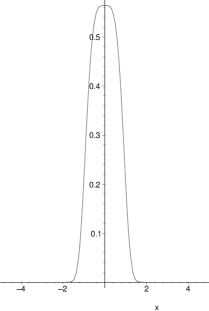
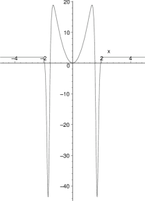
Figure 1: Density and second derivative of $-\log$-density of $\mu_{p}$ for Example 4.5.5 with $p=1/100$ and $a=4$. The second plot reveals a deep multiple wells potential.

4.6 Multivariate mean-difference bound

It is quite natural to ask for a multidimensional counterpart of the mean-difference Lemma 4.3. Let us give some informal ideas to attack this problem. Let $\mu_{0}$ and $\mu_{1}$ be two probability measures on $\mathbb{R}^{d}$, and consider as usual the mixture $\mu_{p}=p\mu_{1}+q\mu_{0}$ with $p\in(0,1)$ and $q=1-p$. It is well known (see for instance [51]) that if $\mu_{0}$ and $\mu_{1}$ are regular enough, then there exists a map $T:\mathbb{R}^{d}\to\mathbb{R}^{d}$ such that the image measure $T\cdot\mu_{0}$ of $\mu_{0}$ by $T$ is $\mu_{1}$ and

$$W_{2}(\mu_{0},\mu_{1})^{2}=\int_{\mathbb{R}^{d}}\!{{\left|T(x)-x\right|}}^{2}\,\mu_{0}(dx).$$

If $\mu_{(s)}$ denotes the image of $\mu_{0}$ by $x\mapsto sT(x)+(1-s)x$ for every $0<s<1$, then

$${{\left(\mathbf{E}_{\mu_{1}}f-\mathbf{E}_{\mu_{0}}f\right)}}^{2}={{\left(\int_{0}^{1}\!\int_{\mathbb{R}^{d}}\!(T(x)-x)\cdot\nabla f(sT(x)+(1-s)x)\,d\mu_{0}(x)\,ds\right)}}^{2}.$$

By Cauchy-Schwarz’s inequality, we get

$${{\left(\mathbf{E}_{\mu_{1}}f-\mathbf{E}_{\mu_{0}}f\right)}}^{2}\leqslant{{\left(\int_{\mathbb{R}^{d}}\!{{\left|T(x)-x\right|}}^{2}\,d\mu_{0}(x)\right)}}{{\left(\int_{0}^{1}\!\int_{\mathbb{R}^{d}}\!{{\left|\nabla f(x)\right|}}^{2}\,d\mu_{(s)}(x)\,ds\right)}}$$

and therefore

$${{\left(\mathbf{E}_{\mu_{1}}f-\mathbf{E}_{\mu_{0}}f\right)}}^{2}\leqslant W_{2}(\mu_{1},\mu_{0})^{2}\int_{\mathbb{R}^{d}}\!\int_{0}^{1}\!{{\left|\nabla f(x)\right|}}^{2}\,d\mu_{(s)}(x)\,ds.$$

This shows that in order to control the mean-difference term ${{\left(\mathbf{E}_{\mu_{1}}f-\mathbf{E}_{\mu_{0}}f\right)}}^{2}$ by $\mathbf{E}_{\mu_{p}}(|\nabla f|^{2})$, it is enough to find a real constant $C_{p}>0$ such that $\overline{\mu}\leqslant C_{p}\mu_{p}$ where

$$\overline{\mu}(A)=\int_{0}^{1}\!\mu_{(s)}(A)\,ds.$$

Unfortunately, this is not feasible if for some $s\in(0,1)$, the support of $\mu_{(s)}$ is not included in the support of $\mu_{p}$ (union of the supports of $\mu_{0}$ and $\mu_{1}$ if $p\in(0,1)$). This problem is due to the linear interpolation used to define $\mu_{(s)}$ via $T$. The linear interpolation will fail if the support of $\mu_{p}$ is a non-convex connected set. Let us adopt an alternative pathwise interpolation scheme. For each $x\in S_{0}=\mathrm{supp}(\mu_{0})$, let us pick a continuous and piecewise smooth interpolating path $\gamma_{x}:[0,1]\to\mathbb{R}^{d}$ such that $\gamma_{x}(0)=x$ and $\gamma_{x}(1)=T(x)$. Then for every smooth $f:\mathbb{R}^{d}\to\mathbb{R}$,

$$f(x)-f(T(x))=\int_{0}^{1}\!\dot{\gamma}_{x}(s)\,\nabla f(\gamma_{x}(s))\,ds\leqslant\sqrt{\int_{0}^{1}\!|\dot{\gamma}_{x}(s)|^{2}\,ds}\ \sqrt{\int_{0}^{1}\!|\nabla f|^{2}(\gamma_{x}(s))\,ds}.$$

As a consequence, we have

$${{\left(\mathbf{E}_{\mu_{0}}f-\mathbf{E}_{\mu_{1}}f\right)}}^{2}\leqslant{{\left(\int_{S_{0}}\!\int_{0}^{1}\!|\dot{\gamma}_{x}(s)|^{2}\,ds\,\mu_{0}(dx)\right)}}\ {{\left(\int_{S_{0}}\!\int_{0}^{1}\!|\nabla f|^{2}(\gamma_{x}(s))\,ds\,\mu_{0}(dx)\right)}}.$$

Now, let $\mu_{(s)}$ be the image measure of $\mu_{0}$ by the map $x\mapsto\gamma_{x}(s)$, where here again $\overline{\mu}$ is the measure defined by $\overline{\mu}(A)=\int_{0}^{1}\!\mu_{(s)}(A)\,ds$. With this notation, we have

$${{\left(\mathbf{E}_{\mu_{0}}f-\mathbf{E}_{\mu_{1}}f\right)}}^{2}\leqslant{{\left(\int_{S_{0}}\!\int_{0}^{1}\!|\dot{\gamma}_{x}(s)|^{2}\,ds\,\mu_{0}(dx)\right)}}\ {{\left(\int_{\mathbb{R}^{d}}\!|\nabla f|^{2}(x)\,\overline{\mu}(dx)\right)}}.$$

Note that

$${{\left(\int_{S_{0}}\!\int_{0}^{1}\!|\dot{\gamma}_{x}(s)|^{2}\,ds\,\mu_{0}(dx)\right)}}\geqslant W_{2}(\mu_{0},\mu_{1})^{2}$$

with equality when $\gamma_{x}$ is the linear interpolation map between $x$ and $T(x)$ for every $x\in S_{0}$. The mean-difference control that we seek for follows then immediately if there exists a real constant $C_{p}>0$ such that $\overline{\mu}\leqslant C_{p}\mu_{p}$. The problem is thus reduced to the choice of an interpolation scheme $\gamma$ such that the support of $\overline{\mu}$ is included in the support of $\mu_{p}$ (which is the union of the supports of $\mu_{0}$ and $\mu_{1}$ as soon as $0<p<1$). Let us give now two enlightening examples.

Example 4.11 (When the linear interpolation map is optimal).

Consider the two-dimensional example where $\mu_{0}=\mathcal{U}([0,2]\times[0,2])$ and $\mu_{1}=\mathcal{U}([1,3]\times[0,2])$. If $\gamma$ is the natural linear interpolation map given by $\gamma_{x}(s)=x+se_{1}$ then $\mu_{(s)}=\mathcal{U}([s,s+2]\times[0,2])$ is supported inside $\mathrm{supp}(\mu_{0})\cup\mathrm{supp}(\mu_{1})$. This is due to the convexity of this union. Also, the linear interpolation map is here optimal. Moreover, elementary computations reveal that

$$C_{p}=\frac{1}{\min(p,q)}\quad\text{and}\quad W_{2}(\mu_{0},\mu_{1})^{2}=1.$$

Therefore, for every $0<p<1$ and any smooth $f:\mathbb{R}^{2}\to\mathbb{R}$,

$${{\left(\mathbf{E}_{\mu_{0}}f-\mathbf{E}_{\mu_{1}}f\right)}}^{2}\leqslant\frac{1}{\min(p,q)}\mathbf{E}_{\mu_{p}}(|\nabla f|^{2}).$$

Example 4.12 (When the linear interpolation map fails).

In contrast, for the example where $\mu_{0}=\mathcal{U}([0,2]\times[0,2])$ and $\mu_{1}=\mathcal{U}([1,3]\times[1,3])$ and if $\gamma$ is the natural linear interpolation map given by $\gamma_{x}(s)=x+s(e_{1}+e_{2})$ then $\mu_{(s)}$ is not supported in $\mathrm{supp}(\mu_{0})\cup\mathrm{supp}(\mu_{1})$ and this union is not convex. If $A=[0,1]\times[2,3]$ then $\mu_{(s)}(A)>0$ for every $0<s<1$ while $\mu_{p}(A)=0$ for every $0<p<1$ and hence there is no finite constant $C_{p}>0$ such that $\overline{\mu}\leqslant C_{p}\mu_{p}$. This shows that the linear interpolation map fails here. Let us give an alternative interpolation map which leads to the desired result. We set for every $x\in\mathrm{supp}(\mu_{0})$ and every $0\leqslant s\leqslant 1$, with $\mathbf{1}=(e_{1},e_{1})$,

$$\gamma_{x}(s)=\begin{cases}(1-s)x+2s\mathbf{1}&\text{if $0\leqslant s\leqslant\frac{1}{2}$}\\ sx+\mathbf{1}&\text{otherwise}.\end{cases}$$

This corresponds to a two-steps linear interpolation between the squares $[0,2]^{2}$ and $[1,3]^{2}$ with intermediate square $[1,2]^{2}$. For every $0\leqslant s\leqslant 1$,

$$\mu_{(s)}=\begin{cases}\mathcal{U}([2s,2]^{2})&\text{if $0\leqslant s\leqslant\frac{1}{2}$}\\ \mathcal{U}([1,1+2s]^{2})&\text{otherwise}.\end{cases}$$

Note that we constructed $\gamma$ in such a way that $\mu_{(s)}$ is always supported in $\mathrm{supp}(\mu_{0})\cup\mathrm{supp}(\mu_{1})$. Elementary computations reveal that for every $0<p<1$,

$$\int_{S_{0}}\!\int_{0}^{1}\!|\dot{\gamma}_{x}(s)|^{2}\,ds\,\mu_{0}(dx)=\frac{8}{3}\quad\text{and}\quad\overline{\mu}\leqslant\frac{4}{\min(p,q)}\mu_{p}.$$

Finally, putting all together, we obtain for every $0<p<1$ and smooth $f:\mathbb{R}^{2}\to\mathbb{R}$,

$${{\left(\mathbf{E}_{\mu_{0}}f-\mathbf{E}_{\mu_{1}}f\right)}}^{2}\leqslant\frac{32}{3\min(p,q)}\mathbf{E}_{\mu_{p}}(|\nabla f|^{2}).$$

As a conclusion, one can retain that the natural interpolation problem associated to the control of the mean-difference involves a kind of support-constrained interpolation for mass transportation.

Acknowledgements. The authors would like to warmly thank Arnaud Guillin, Sébastien Gouëzel, and all the participants of the Working Seminar Inégalités fonctionnelles held on March 2008 at the Institut Henri Poincaré of Paris for fruitful discussions. The final form of the paper has benefited from the fine comments of two anonymous reviewers.

Compiled

Djalil Chafaï mailto:chafai(AT)math.univ-toulouse.fr

UMR181 INRA ENVT, 23 Chemin des Capelles F-31076 Toulouse Cedex 3, France.

UMR5583 CNRS Institut de Mathématiques de Toulouse (IMT)
Université de Toulouse III, 118 route de Narbonne, F-31062, Toulouse Cedex, France.

Florent Malrieu mailto:florent.malrieu(AT)univ-rennes1.fr

UMR 6625 CNRS Institut de Recherche Mathématique de Rennes (IRMAR)
Université de Rennes I, Campus de Beaulieu, F-35042 Rennes Cedex, France.

References

- [1] C. Ané, S. Blachère, D. Chafaï, P. Fougères, I. Gentil, F. Malrieu, C. Roberto, and G. Scheffer, Sur les inégalités de Sobolev logarithmiques, Société Mathématique de France, Paris, 2000, Preface by D. Bakry and M. Ledoux.
- [2] D. Bakry and M. Émery, Diffusions hypercontractives, Séminaire de probabilités, XIX, 1983/84, Lecture Notes in Math., vol. 1123, Springer, Berlin, 1985, pp. 177–206.
- [3] D. Bakry, M. Ledoux, and F.-Y. Wang, Perturbations of functional inequalities using growth conditions, J. Math. Pures Appl. (9) 87 (2007), no. 4, 394–407.
- [4] F. Barthe, P. Cattiaux, and C. Roberto, Interpolated inequalities between exponential and Gaussian, Orlicz hypercontractivity and isoperimetry, Rev. Mat. Iberoam. 22 (2006), no. 3, 993–1067.
- [5] F. Barthe and C. Roberto, Sobolev inequalities for probability measures on the real line, Studia Math. 159 (2003), no. 3, 481–497, Dedicated to Professor Aleksander Pełczyński on the occasion of his 70th birthday (Polish).
- [6] S. G. Bobkov, Concentration of normalized sums and a central limit theorem for noncorrelated random variables, Ann. Probab. 32 (2004), no. 4, 2884–2907.
- [7] , Generalized symmetric polynomials and an approximate de Finetti representation, J. Theoret. Probab. 18 (2005), no. 2, 399–412.
- [8] S. G. Bobkov and F. Götze, Exponential integrability and transportation cost related to logarithmic Sobolev inequalities, J. Funct. Anal. 163 (1999), no. 1, 1–28.
- [9] F. Bolley and C. Villani, Weighted Csiszár-Kullback-Pinsker inequalities and applications to transportation inequalities, Ann. Fac. Sci. Toulouse (2005), 331–352.
- [10] L. A. Caffarelli, Monotonicity properties of optimal transportation and the FKG and related inequalities, Comm. Math. Phys. 214 (2000), no. 3, 547–563.
- [11] , Erratum: [Comm. Math. Phys. 214 (2000), no. 3, 547–563], Comm. Math. Phys. 225 (2002), no. 2, 449–450.
- [12] E. A. Carlen, Superadditivity of Fisher’s information and logarithmic Sobolev inequalities, J. Funct. Anal. 101 (1991), no. 1, 194–211.
- [13] S. Chatterjee, Spin glasses and Stein’s method, preprint arXiv:0706.3500v2 [math.PR], 2007.
- [14] P. Diaconis and L. Saloff-Coste, Logarithmic Sobolev inequalities for finite Markov chains, Ann. Appl. Probab. 6 (1996), no. 3, 695–750.
- [15] H. Djellout, A. Guillin, and L. Wu, Transportation cost-information inequalities and applications to random dynamical systems and diffusions, Ann. Probab. 32 (2004), no. 3B, 2702–2732.
- [16] B. S. Everitt and D. J. Hand, Finite mixture distributions, Chapman & Hall, London, 1981, Monographs on Applied Probability and Statistics.
- [17] V. P. Fonf, J. Lindenstrauss, and R. R. Phelps, Infinite dimensional convexity, Handbook of the geometry of Banach spaces, Vol. I, North-Holland, Amsterdam, 2001, pp. 599–670.
- [18] S. Frühwirth-Schnatter, Finite mixture and Markov switching models, Springer Series in Statistics, Springer, New York, 2006.
- [19] I. Gentil, Inégalités de Sobolev logarithmique et de Poincaré pour la loi uniforme, unpublished note, available on the author’s web page, 2004.
- [20] I. Gentil and C. Roberto, Spectral gaps for spin systems: some non-convex phase examples, J. Funct. Anal. 180 (2001), no. 1, 66–84.
- [21] N. Gozlan, A characterization of dimension free concentration in terms of transportation inequalities, preprint arXiv: 0804.3089 [math.PR], 2008.
- [22] M. Gromov and V. D. Milman, A topological application of the isoperimetric inequality, Amer. J. Math. 105 (1983), no. 4, 843–854.
- [23] L. Gross, Logarithmic Sobolev inequalities, Amer. J. Math. 97 (1975), no. 4, 1061–1083.
- [24] , Hypercontractivity, logarithmic Sobolev inequalities, and applications: a survey of surveys, Diffusion, quantum theory, and radically elementary mathematics, Math. Notes, vol. 47, Princeton Univ. Press, Princeton, NJ, 2006, pp. 45–73.
- [25] B. Helffer, Semiclassical analysis, Witten Laplacians, and statistical mechanics, Series in Partial Differential Equations and Applications, vol. 1, World Scientific Publishing Co. Inc., River Edge, NJ, 2002.
- [26] W. Hoeffding, Probability inequalities for sums of bounded random variables, J. Amer. Statist. Assoc. 58 (1963), 13–30.
- [27] R. Holley and D. Stroock, Logarithmic Sobolev inequalities and stochastic Ising models, J. Statist. Phys. 46 (1987), no. 5-6, 1159–1194.
- [28] M. Jerrum, J.-B. Son, P. Tetali, and E. Vigoda, Elementary bounds on Poincaré and log-Sobolev constants for decomposable Markov chains, Ann. Appl. Probab. 14 (2004), no. 4, 1741–1765.
- [29] O. Johnson, Convergence of the Poincaré constant, Teor. Veroyatnost. i Primenen. 48 (2003), no. 3, 615–620, preprint version available at arXiv.org:math.PR/0206227.
- [30] I. Kontoyiannis and M. Madiman, Measure concentration for compound Poisson distributions, Electron. Comm. Probab. 11 (2006), 45–57 (electronic).
- [31] L. Kontoyiannis and M. Madiman, Entropy, compound Poisson approximation, log-Sobolev inequalities and measure concentration, Information Theory Workshop,24–29 Oct. 2004. IEEE, 2004, pp. 71–75.
- [32] R. Latała, On some inequalities for Gaussian measures, Proceedings of the International Congress of Mathematicians, Vol. II (Beijing, 2002) (Beijing), Higher Ed. Press, 2002, pp. 813–822.
- [33] M. Ledoux, Concentration of measure and logarithmic Sobolev inequalities, Séminaire de Probabilités, XXXIII, Springer, Berlin, 1999, pp. 120–216.
- [34] , The concentration of measure phenomenon, Mathematical Surveys and Monographs, vol. 89, American Mathematical Society, Providence, RI, 2001.
- [35] N. Madras and D. Randall, Markov chain decomposition for convergence rate analysis, Ann. Appl. Probab. 12 (2002), no. 2, 581–606.
- [36] K. Marton, A simple proof of the blowing-up lemma, IEEE Trans. Inform. Theory 32 (1986), no. 3, 445–446.
- [37] , Bounding -distance by informational divergence: a method to prove measure concentration, Ann. Probab. 24 (1996), no. 2, 857–866.
- [38] V. G. Maz’ja, Sobolev spaces, Springer Series in Soviet Mathematics, Springer-Verlag, Berlin, 1985, Translated from the Russian by T. O. Shaposhnikova.
- [39] G. McLachlan and K. Basford, Mixture models, Statistics: Textbooks and Monographs, vol. 84, Marcel Dekker Inc., New York, 1988, Inference and applications to clustering.
- [40] G. McLachlan and D. Peel, Finite mixture models, Wiley Series in Probability and Statistics: Applied Probability and Statistics, Wiley-Interscience, New York, 2000.
- [41] L Miclo, Quand est-ce que des bornes de Hardy permettent de calculer une constante de Poincaré exacte sur la droite ?, preprint, http://hal.archives-ouvertes.fr/hal-00017875/en/, 2005.
- [42] F. Otto and M. G. Reznikoff, A new criterion for the logarithmic Sobolev inequality and two applications, J. Funct. Anal. 243 (2007), no. 1, 121–157.
- [43] R. R. Phelps, Lectures on Choquet’s theorem, second ed., Lecture Notes in Mathematics, vol. 1757, Springer-Verlag, Berlin, 2001.
- [44] S. T. Rachev, Probability metrics and the stability of stochastic models, Wiley Series in Probability and Mathematical Statistics: Applied Probability and Statistics, John Wiley & Sons Ltd., Chichester, 1991.
- [45] L. Saloff-Coste, Lectures on finite Markov chains, Lectures on probability theory and statistics (Saint-Flour, 1996), Lecture Notes in Math., vol. 1665, Springer, Berlin, 1997, pp. 301–413.
- [46] A. J. Stam, Some inequalities satisfied by the quantities of information of Fisher and Shannon, Information and Control 2 (1959), 101–112.
- [47] V. N. Sudakov, Geometric problems in the theory of infinite-dimensional probability distributions, Proc. Steklov Inst. Math. (1979), no. 2, i–v, 1–178, Cover to cover translation of Trudy Mat. Inst. Steklov 141 (1976).
- [48] A. Takatsu, On Wasserstein geometry of the space of Gaussian measures, arXiv:0801.2250 [math.DG], 2008.
- [49] M. Talagrand, Transportation cost for Gaussian and other product measures, Geom. Funct. Anal. 6 (1996), no. 3, 587–600.
- [50] D. M. Titterington, A. F. M. Smith, and U. E. Makov, Statistical analysis of finite mixture distributions, Wiley Series in Probability and Mathematical Statistics: Applied Probability and Statistics, John Wiley & Sons Ltd., Chichester, 1985.
- [51] C. Villani, Topics in optimal transportation, Graduate Studies in Mathematics, vol. 58, American Mathematical Society, Providence, RI, 2003.
- [52] , Optimal transport, old and new, lecture notes, École d’été de Saint-Flour 2005, preprint, 2007.