Phase diagram of the Ising square lattice with competing interactions

Abstract

We restudy the phase diagram of the 2D-Ising model with competing interactions $J_{1}$ on nearest neighbour and $J_{2}$ on next-nearest neighbour bonds via Monte-Carlo simulations. We present the finite temperature phase diagram and introduce computational methods which allow us to calculate transition temperatures close to the critical point at $J_{2}=J_{1}/2$. Further on we investigate the character of the different phase boundaries and find that the transition is weakly first order for moderate $J_{2}>J_{1}/2$.

1 Introduction

The search for exotic groundstates in two-dimensional frustrated quantum spin systems is a topic of intense research (see, e.g., Refs. P:misguich05 ; P:richter04 for recent reviews). In this context, the antiferromagnetic $J_{1}$-$J_{2}$ spin-1/2 Heisenberg model on the square lattice has been intensively studied during the past two decades. Nevertheless, the nature of an intermediate non-magnetic phase around $J_{2}\approx J_{1}/2$ has remained under debate until recently (see Refs. P:misguich05 ; P:mambrini06 and references therein). Among the possible approaches to the antiferromagnetic $J_{1}$-$J_{2}$ Heisenberg model, quantum Monte-Carlo (QMC) simulations suffer from a severe sign problem in the region $J_{2}\approx J_{1}/2$. Other approaches include perturbation theory around the Ising limit P:oitmaa96 ; P:singh03 . A closely related model is given by hard-core bosons on the square lattice with nearest neighbour (NN) and next-nearest neighbour (NNN) hopping and repulsion terms P:batrouni00 ; P:batrouni01 ; P:wessel08 ; P:chen08 . In this case, there is no sign problem such that QMC simulations are possible in principle P:batrouni00 ; P:batrouni01 ; P:wessel08 ; P:chen08 . However, simple QMC algorithms suffer freezing problems in the intermediate regime at $J_{2}=J_{1}/2$ which can be traced to a groundstate degeneracy of the Ising limit. This motivated us to perform a model study by solving the related freezing problems in Monte-Carlo (MC) simulations of the Ising model.

Investigations of the two-dimensional $J_{1}$-$J_{2}$ Ising model on the square lattice have an even longer history than of the corresponding Heisenberg model, including in particular MC simulations (see, e.g., P:SK79 ; P:landau80 ; P:landaubinder80 ; P:landaubinder85 ; P:bloete87 ; P:MKT06 ; B:landaubinder ). Nevertheless, certain issues have remained controversial also in the case of the Ising model, in particular the nature of the finite-temperature phase transition for $J_{2}>J_{1}/2$: MC simulations P:SK79 ; P:landaubinder85 ; P:MKT06 and an investigation of the Fisher zeros of the partition function P:monroe07 have suggested non-universal critical exponents, whereas a variational approach P:lopez93 and a differential operator technique P:AVS08 predict a first-order transition for $J_{1}/2<J_{2}\lesssim J_{1}$. In this paper we resolve this issue in favour of a weak first-order transition at least for not too large $J_{2}>J_{1}/2$ by providing substantially improved MC results for the phase diagram.

This paper is organized as follows: in section 1.1 we introduce the $J_{1}$-$J_{2}$ Ising model on the square lattice and discuss its $T=0$ groundstates. The MC simulation methods are described in section 2 and results are presented in section 3. We conclude with a summary and outlook in section 4.

1.1 Model

We study the classical Ising model with competing antiferromagnetic interactions $J_{1}$ on the NN bonds and $J_{2}$ on the NNN bonds ($J_{i}>0$):

$$H=J_{1}\sum_{\text{NN}}S_{i}S_{j}+J_{2}\sum_{\text{NNN}}S_{i}S_{j}\,,\quad S_{i}=\pm 1\,.$$ (1)

We will study square lattices of linear extent $L$ with periodic boundary conditions.

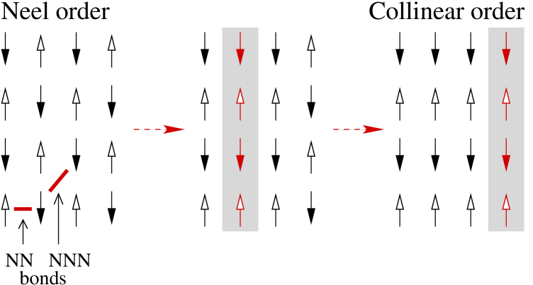
Figure 1: Sketched are both ordered phases and a third groundstate configuration at $J_{2}=J_{1}/2$ (middle). The total degeneracy of the groundstate at $J_{2}=J_{1}/2$ is of order $2^{L+1}$. Shaded areas mark flipped lines.

For $J_{2}=0$ the groundstate of (1) is the known antiferromagnetic solution which is a Néel ordered lattice (see Fig. 1, left) with energy $E=-2J_{1}N$ ($N=L^{2}$ is the number of sites). Switching on the repulsive interaction on the diagonal (NNN) bonds of the square lattice yields an increase of the groundstate energy for the Néel-ordered state:

$$E_{\text{N\'{e}el}}=-2N(J_{1}-J_{2})\,.$$ (2)

For large $J_{2}$ the system orders in the collinear (or superantiferromagnetic) phase (see Fig. 1, right) where all diagonal bonds are antiferromagnetic, while half of the NN bonds is antiferromagnetic and the other half is ferromagnetic. Thus, the energy in this state depends only on $J_{2}$:

$$E_{\text{Coll}}=-2NJ_{2}\,.$$ (3)

The critical point separating these two phases lies at $J_{2}=J_{1}/2$, where the transition temperature is suppressed to $T=0$. At this point the groundstate is highly degenerate. More precisely, there are $2^{L+1}-2$ groundstates which can be obtained as follows: flipping a line of antiparallel spins costs no energy at $J_{2}=J_{1}/2$. Thus, one can generate almost $2^{L+1}$ groundstates from a Néel state by flipping either the $L$ horizontal or the $L$ vertical lines independently (the second Néel state can be reached in both ways). In particular, one can reach a collinear state through a series of intermediate groundstates by $L/2$ line flips, as sketched in Fig. 1. Accordingly, close to the critical point $J_{2}=J_{1}/2$ the energy landscape is characterized by many local minima which are separated by large energy barriers. Therefore, MC simulations using only single-spin flips have problems to reach the configuration with global minimum energy. To solve this problem and to obtain transition temperatures also in the vicinity of $J_{2}=J_{1}/2$ we implemented improved MC algorithms which we will discuss in the next section.

2 Methods

2.1 Computational methods

We first tried to simulate the model with competing interactions using conventional single-spin flip MC simulations B:landaubinder . However, near the critical point this algorithm does not provide proper results and suffers severe freezing problems in the proximity of the critical temperature and below. To overcome these problems we implemented a parallel tempering algorithm P:huku96 ; P:marinari98 ; P:hans97 ; P:trebst06 : a number of simulations with the same set of parameters ($J_{1}$, $J_{2}$, $L$) but varying temperatures are simulated simultaneously. After a sufficiently large number of sweeps over the complete lattice an additional MC step proposes a configuration swap between neighbouring simulations with an acceptance rate $p(i,i+1)$:

$$p(i,i+1)=\min\left\{1,e^{\Delta\beta\Delta E}\right\}\,,$$ (4)

$$\Delta\beta=\frac{1}{T_{i+1}}-\frac{1}{T_{i}}\,,\quad\Delta E=E_{i+1}-E_{i}\,.$$

We have chosen the temperatures $T_{i}$ logarithmically with a density maximum near the estimated transition temperature. A selfadjusting temperature set P:trebst06 was not necessary for our purposes. To manage the additional computational workload of the parallel tempering algorithm we implemented a parallelisation of the MC code via OpenMP B:omp00 ; B:omp07 . To assure the independence of the simulations we used the sprng (version 4.0) P:masca00 lagged Fibonacci generator for producing independent random number streams for each simulation. We have checked in some samples that our MC results do not change if we replace the random number generator by the Mersenne Twister algorithm P:matsu98 , as implemented in the boost libraries version 1.33.1.

Another way to improve the MC simulations is to allow not only single-spin updates but also flipping whole lines of spins in an additional MC step (as sketched in Fig. 1). This method simulates directly the transition between degenerate groundstates at $J_{2}=J_{1}/2$ and helps to minimize statistical errors for lattice sizes up to $50\times 50$. For larger lattices the probability to flip a whole line decreases rapidly for ratios $J_{2}\neq J_{1}/2$ while the simulation time to calculate them increases with $L$. We also tried cluster updates P:wolff89 but in the case of competing interactions this method does not help: when one approaches the critical temperature, the clusters extend over the whole lattice and therefore do not support the ordering process.

The parallel tempering algorithm gives rise to correlations between different temperature points in a simulation which can affect the independency of the calculated data. Therefore, the meanvalues and errorbars of the shown observables are derived from at least 10 independent MC runs.

2.2 Order parameters

To distinguish the two ordered and the disordered phases we use the respective structure factors

$$S(\vec{q})=\frac{1}{N}\sum_{i,j}e^{i\vec{q}\cdot(\vec{x}_{i}-\vec{x}_{j})}\langle S_{i}S_{j}\rangle$$ (5)

where $\vec{q}$ is a vector in momentum space and indicates the different magnetic phases:

$$\vec{q}=(0,0) \rightarrow$$ ferromagnetic order,

$$\vec{q}=(0,\pi),(\pi,0) \rightarrow$$ collinear order, (6)

$$\vec{q}=(\pi,\pi) \rightarrow$$ Néel order.

We identify $M(\vec{q})=\sqrt{S(\vec{q})/N}$ as our order parameter. The Néel order parameter can be calculated as staggered magnetization due to a simple sublattice rotation. Using the order of the collinear phase we can also calculate the associated order parameter via the column or line index of the underlying lattice. To find the transition temperature we calculate the fourth order Binder cumulant P:binder81a ; P:binder81b ; B:landaubinder for different system sizes $L$:

$$U_{4}=1-\frac{\langle M^{4}\rangle}{3\langle M^{2}\rangle^{2}}\,.$$ (7)

For large enough $L$ they will meet in a single point at $T_{C}$ (for an example see Fig. 2).

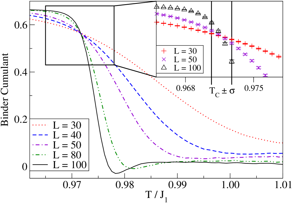
Figure 2: Binder cumulants depending on temperature for $J_{2}=0.6J_{1}$ and different lattice sizes. In the inset three cumulants are plotted with errorbars. The intersection area gives $T_{C}$ with small error.

To analyze the character of the phase transition we calculated the specific heat and recorded time series of the energies to set up histograms P:challa86 ; P:berg91 ; P:borgs92 . Furthermore we calculated the temperature derivative of the Binder cumulant which is related with the critical exponent $\nu$ B:landaubinder to study the critical behaviour of the system:

$$aL^{1/\nu}=\left.\frac{\partial U_{4}}{\partial T}\right|_{T=T_{C}}\,.$$ (8)

To have a closer look on the critical point $J_{2}=J_{1}/2$ we analyzed the peaks of the specific heat via polynomial fitting.

3 Results

We calculated the critical temperatures for various ratios of $J_{2}/J_{1}$ especially close to the critical point (Fig. 3). Our data is in good agreement with MC results from Landau and Binder for $J_{2}\geq 0.6J_{1}$ P:landaubinder85 and $J_{2}\leq 0.4J_{1}$ P:landau80 . In addition, our improved MC algorithm with the above described parallel tempering mode and line flip updates enabled us to obtain results much closer to $J_{2}=J_{1}/2$ ($|J_{2}/J_{1}-0.5|=0.005$) for system sizes up to $N=250\leavevmode\nobreak\ 000$.

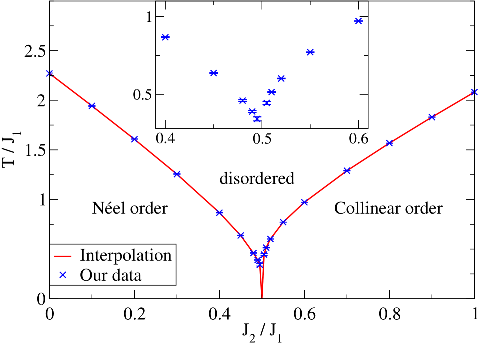
Figure 3: Plotted are $T_{C}$’s over the ratio $J_{2}/J_{1}$. Data were produced by parallel tempering MC simulations. Near the critical point $J_{2}=J_{1}/2$ additional line flip updates led to a better convergence.

To investigate the character of the phase transition we calculated the specific heat and energy histograms for different lattice sizes. Looking at the peaks in the specific heat for different $J_{2}/J_{1}$ suggests different character of the phase transition. For $J_{2}<J_{1}/2$ (Fig. 4(a)) we have a slowly emerging peak with growing system size. Indeed, for an Ising like transition we expect only a logarithmic divergence in the specific heatP:onsager44 and a critical exponent $\nu=1$ P:fisher67 . To verify the Ising like behaviour we had a closer look at the derivative of the Binder cumulant $U_{4}$ near the critical temperature. We expect a linear correspondence in $L$ for equation (8). An analysis of our results at $J_{2}=0.3J_{1}$ yields $\nu=0.99(1)$ which is in good agreement with the expected value $\nu=1$. On the other hand for $J_{2}>J_{1}/2$ and in particular for the case $J_{2}=0.6J_{1}$ shown in Fig. 4(b) there are different opinions about the character of the phase transition. Some authors assume a continuous phase transition with non universal exponents P:SK79 ; P:landaubinder85 ; P:MKT06 ; P:monroe07 whereas other authors find a first order phase transition P:lopez93 ; P:AVS08 . Note that our results for the specific heat (Fig. 4(b)) differ quantitatively from the approximate results of P:lopez93 . In particular, the maximum of the specific heat continues to diverge for growing $L$. We estimated the area under the peak in dependence on the lattice size and find it to converge towards a constant value for large enough $L$. This indicates a $\delta$-peak structure for the specific heat in the thermodynamic limit as expected for a first order phase transition. We should nevertheless mention that the value of the specific heat does not follow the finite size scaling law expected for first order transitions P:challa86 very well, which may be due to crossover phenomena.

As further verification of our characterisation of the order of the phase transition we computed energy histograms. First, we extracted a system-size dependent $T_{C}$ from the maximum of the specific heat. Then we recorded the time series of the energy for each system size and the associated $T_{C}$. Fig. 5 shows the resulting energy distribution for $J_{2}=0.3J_{1}$ and $J_{2}=0.6J_{1}$. For $J_{2}=0.3J_{1}$ we find a single peak, consistent with a conventional second order phase transition. By contrast, for $J_{2}=0.6J_{1}$ a double peak structure emerges for sufficiently large system size, see Fig. 5(b). Such a double peak structure is characteristic for a first order transition P:challa86 ; P:berg91 ; P:borgs92 . The fact that the double peak structure emerges only for large system sizes shows that the transition for $J_{2}=0.6J_{1}$ is a weak first order one. Since we have observed similar behavior for nearby ratios of $J_{2}/J_{1}$, we believe the transition for $J_{2}>J_{1}/2$ to be of first order, at least for not too large values of $J_{2}$.

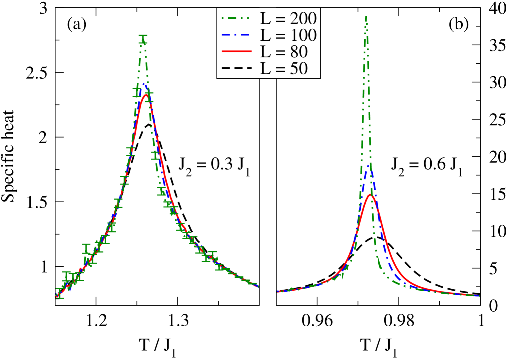
Figure 4: Comparison of specific heats for $J_{2}<J_{1}/2$ (a) and $J_{2}>J_{1}/2$ (b). The peaks emerge at the critical temperature obtained from the fourth order cumulant calculations. Note the different magnitudes of the divergence. Errorbars are omitted if they are of the same order as the linewidth.

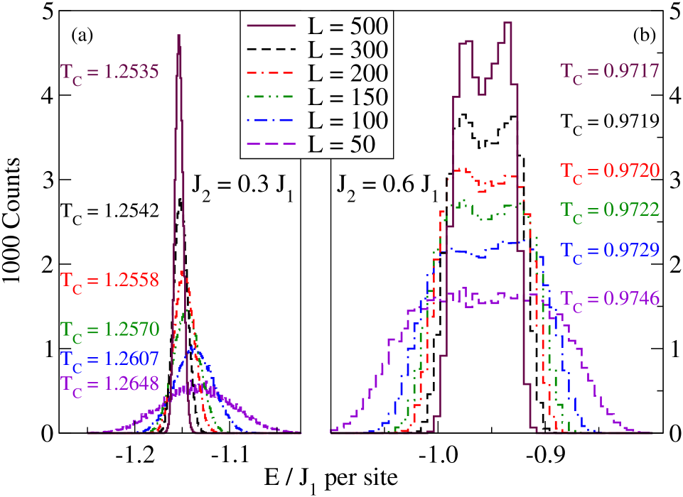
Figure 5: Energy histogram for $J_{2}=0.3J_{1}$ ($binsize=10^{-4}J_{1}$) and $J_{2}=0.6J_{1}$ ($binsize=6\cdot 10^{-3}J_{1}$). For each lattice size $L$ the histogram is plotted at the critical temperature $T_{C}(L)$. The slowly emerging double peak structure in panel (b) in comparison to the clearly single peaked structure in panel (a) indicates a weak first order transition for $J_{2}>J_{1}/2$.

Fig. 6 shows the specific heat exactly at the critical point $J_{2}=J_{1}/2$ for different system sizes. The purpose of this computation is to verify if a direct phase transition from Néel to collinear order is possible at finite temperature, or if any other finite-temperature phase could exist in this region. Previous publications P:landau80 ; P:lopez93 have shown curves for the specific heat at $J_{2}=J_{1}/2$ with a rounded peak, but we are not aware of any systematic finite-size analysis. In our results, we observe that the peaks of the specific heat are moving to lower temperatures for increasing system sizes, suggesting that the transition temperature is suppressed to $T_{C}=0$ in the thermodynamic limit. To further substantiate this conclusion, the inset of Fig. 6 shows the peak positions ($T_{C}$) with respect to the inverse lattice length $1/L$. For the given lattice sizes we find a power law behaviour for $T_{C}$ and $1/L$. This is consistent with $T_{C}=0$ in the thermodynamic limit.

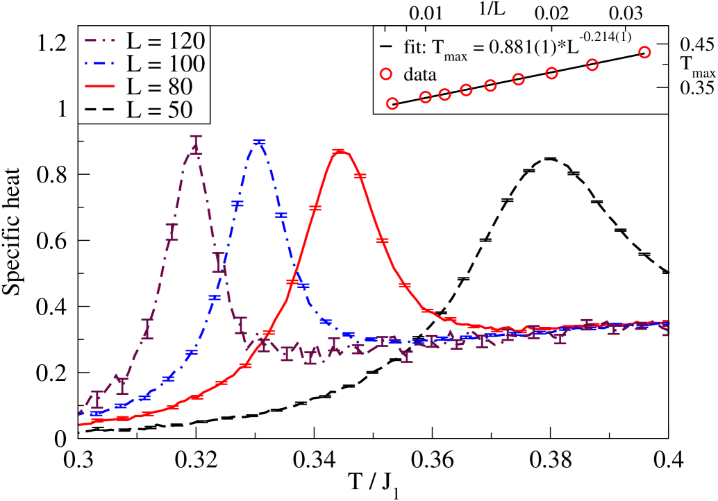
Figure 6: Specific heat at $J_{2}=0.5J_{1}$ for different lattice sizes with errorbars at every fourth data point. The peak moves towards lower temperature (here $T_{C}/J_{1}=0.380(4),0.345(4),0.331(3),0.320(2)$) for growing system sizes. The inset shows $T_{C}$ (obtained from a polynomial fitting of the maximum in the specific heat) versus the inverse lattice length in a log-log-scale (errorbars are smaller than the symbols). The behaviour of $T_{C}$ is consistent with a power law in $L$, indicating $T_{C}=0$ in the thermodynamic limit.

4 Discussion

In this paper, we combined single-spin flip, parallel tempering and line flip MC algorithms to enhance the efficiency of MC simulations of the frustrated square-lattice Ising model. These improvements enabled us to compute critical temperatures in the direct vicinity of the critical point $J_{2}=J_{1}/2$ where the groundstate is highly degenerate. For $J_{2}<J_{1}/2$ there is a finite-temperature phase transition into a Néel-ordered state. This transition belongs to the two-dimensional Ising universality class. We believe that at the critical point $J_{2}=J_{1}/2$ the transition temperature is suppressed to zero. On the right hand side ($J_{2}>J_{1}/2$) there is again a finite-temperature phase transition into a phase with collinear order.

At $J_{2}=0.6J_{1}$ we have observed a double peak structure in the histogram of the energy. This identifies the phase transition as a weakly first order one. We believe this first order transition to be generic for moderate $J_{2}>J_{1}/2$. However, for larger $J_{2}$ it becomes increasingly difficult to identify a double peak structure in the histogram of the energy. Therefore, the transition could in fact become a second order one for $J_{2}\gtrsim J_{1}$. Note that a recent MC investigation P:MKT06 has concluded that the transition is second order for $J_{2}=J_{1}$, although in P:MKT06 only smaller lattices have been considered than in the present work.

In order to understand the possible nature of the transition at large $J_{2}$, it is instructive to consider the limit $J_{1}=0$ where one has two decoupled Ising models. The critical theory then consists of two conformal field theories with central charge $c=1/2$ each, i.e., a $c=1$ theory. Thus, the point $J_{1}=0$ lies within the manifold of $c=1$ conformal field theories where continuously varying critical exponents are possible in principle P:ginsparg88 . However, the coupling given by $J_{1}$ turns out to be a relevant perturbation of the critical point such that this coupling should either lead to a first order transition or a fixed point with $c<1$ B:cardy96 . According to the classification of minimal conformal field theories with $c<1$ P:BPZ84 a possible second order phase transition at $J_{2}\gg J_{1}$ should have universal exponents. Therefore, a scenario with non-universal critical behaviour P:SK79 ; P:landaubinder85 ; P:MKT06 ; P:monroe07 does not appear very plausible from a conformal field theory perspective either. Our MC results show that large crossover scales exist in the present model such that very big lattices would be needed for a reliable numerical determination of the nature of the transition for $J_{2}\gtrsim J_{1}$.

A similar phase diagram as in the Ising model is also found for the classical $J_{1}$-$J_{2}$ $X$-$Y$ P:simon00 and Heisenberg models P:weber03 . However, we believe that the nature of the phase transition for $J_{2}>J_{1}/2$ is a different issue in these two models due to the different symmetries in spin space.

After having solved the freezing problems in the Ising model, we are now about to introduce hopping terms and to study finite-temperature properties of hard-core bosons on the square lattice using parallel tempering QMC simulations P:melko07 .

- (1) G. Misguich, C. Lhuillier, in Frustrated spin systems, edited by H.T. Diep (World-Scientific, 2005)
- (2) J. Richter, J. Schulenburg, A. Honecker, in Quantum Magnetism, edited by U. Schollwöck, J. Richter, D.J.J. Farnell, R.F. Bishop, (Lecture Notes in Physics, 645) (Springer, Berlin, 2004) p. 85
- (3) M. Mambrini, A. Läuchli, D. Poilblanc, F. Mila, Phys. Rev. B 74, 144422 (2006)
- (4) J. Oitmaa, Zheng Weihong, Phys. Rev. B 54, 3022 (1996)
- (5) R.R.P. Singh, W. Zheng, J. Oitmaa, O.P. Sushkov, C.J. Hamer, Phys. Rev. Lett. 91, 017201 (2003)
- (6) G.G. Batrouni, R.T. Scalettar, Phys. Rev. Lett. 84, 1599 (2000)
- (7) F. Hébert, G.G. Batrouni, R.T. Scalettar, G. Schmid, M. Troyer, A. Dorneich, Phys. Rev. B 65, 014513 (2001)
- (8) Y.-C. Chen, R.G. Melko, S. Wessel, Y.-J. Kao, Phys. Rev. B 77, 014524 (2008)
- (9) K.-K. Ng, Y.-C. Chen, Phys. Rev. B 77, 052506 (2008)
- (10) R.H. Swendsen, S. Krinsky, Phys. Rev. Lett. 43, 177 (1979)
- (11) D.P. Landau, Phys. Rev. B 21, 1285 (1980)
- (12) K. Binder, D.P. Landau, Phys. Rev. B 21, 1941 (1980)
- (13) D.P. Landau, K. Binder, Phys. Rev. B 31, 5946 (1985)
- (14) H.W.J. Blöte, A. Compagner, A. Hoogland, Physica A 141, 375 (1987)
- (15) A. Malakis, P. Kalozoumis, N. Tyraskis, Eur. Phys. J. B 50, 63 (2006)
- (16) D.P. Landau, K. Binder, Monte Carlo Simulations in Statistical Physics (Cambridge University Press, 2000)
- (17) J.L. Monroe, S. Kim, Phys. Rev. E 76, 021123 (2007)
- (18) J.L. Morán-López, F. Aguilera-Granja, J.M. Sanchez, Phys. Rev. B 48, 3519 (1993)
- (19) R.A. dos Anjos, J.R. Viana, J.R. de Sousa, Phys. Lett. A 372, 1180 (2008)
- (20) K. Hukushima, K. Nemoto, J. Phys. Soc. Jpn. 65, 1604 (1996)
- (21) E. Marinari, Lecture Notes in Physics, 501, 50 (Springer, 1998) [cond-mat/9612010]
- (22) U.H.E. Hansmann, Chem. Phys. Lett. 281, 140 (1997)
- (23) H.G. Katzgraber, S. Trebst, D.A. Huse, M. Troyer, J. Stat. Mech., P03018 (2006)
- (24) B. Chapman, G. Jost, R. v. d. Pas, Using OpenMP: Portable Shared Memory Parallel Programming (The MIT Press, 2007)
- (25) R. Chandra, R. Menon, L. Dagum, D. Kohr, D. Maydan, J. McDonald, Parallel Programming in OpenMP (Morgan Kaufmann, 2000)
- (26) M. Mascagni, A. Srinivasan, ACM TOMS 26, 436 (2000)
- (27) M. Matsumoto, T. Nishimura, ACM TOMACS 8, 3 (1998)
- (28) U. Wolff, Phys. Rev. Lett. 62, 361 (1989)
- (29) K. Binder, Phys. Rev. Lett. 47, 693 (1981)
- (30) K. Binder, Z. Phys. B 43, 119 (1981)
- (31) M.S.S. Challa, D.P. Landau, K. Binder, Phys. Rev. B 34, 1841 (1986)
- (32) N.A. Alves, B.A. Berg, R. Villanova, Phys. Rev. B 43, 5846 (1991)
- (33) C. Borgs, W. Janke, Phys. Rev. Lett. 68, 1738 (1992)
- (34) L. Onsager, Phys. Rev. 65, 117 (1944)
- (35) M.E. Fisher, R.J. Burford, Phys. Rev. 156, 583 (1967)
- (36) P. Ginsparg, Nucl. Phys. B 295, 153 (1988)
- (37) J. Cardy, Scaling and Renormalization in Statistical Physics (Cambridge University Press, Cambridge, 1996)
- (38) A.A. Belavin, A.M. Polyakov, A.B. Zamolodchikov, Nucl. Phys. B 241, 333 (1984)
- (39) D. Loison, P. Simon, Phys. Rev. B 61, 6114 (2000)
- (40) C. Weber, L. Capriotti, G. Misguich, F. Becca, M. Elhajal, F. Mila, Phys. Rev. Lett. 91, 177202 (2003)
- (41) R.G. Melko, J. Phys.: Condens. Matter 19, 145203 (2007)