Statistical Modeling of Solar Flare Activity from
Empirical Time Series of Soft X-ray Solar Emission

Abstract

A time series of soft X-ray emission observed on 1974-2007 years (GOES) is analyzed. We show that in the periods of high solar activity 1977-1981, 1988-1992, 1999-2003 the energy statistics of soft X-ray solar flares for class M and C is well described by a FARIMA time series with Pareto innovations. The model is characterized by two effects. One of them is a long-range dependence (long-term memory), and another corresponds to heavy-tailed distributions. Their parameters are statistically stable enough during the periods. However, when the solar activity tends to minimum, they change essentially. We discuss possible causes of this evolution and suggest a statistical model for predicting the flare energy statistics.

1 Introduction

Individual solar cycles are different in form, amplitude and length. At present, the accurate solar data is only available for the most recent three cycles. Understanding the long-term solar variability and predicting the solar activity is an actual problem for solar physics. It is very important to predict the time and strength of such events because these disturbances can pose serious threats to man-made spacecrafts, can disrupt electronic communication channels and can even set up huge electrical currents in power grids (Clark 2006). It is enough to remind about serious problems with GOES, Deuthsche Telecom, Telstars 401, etc. Satellite operators would be glad to escape the unhappy surprise, and mission planners are compelled to take into account the future space weather forecast. Not only NASA satellites malfunctioned because of the disturbances, but the global positioning system was impaired. The cost to the airline industry arose as planes were re-routed to lower altitudes, burning more fuel in force of atmospheric drag.

As the geological records show, the Earth’s climate has always been changing. The reasons for such changes, however, have always been subject to continuous discussions and are still not well understood. In addition to natural climate changes the risk of human influence on climate is seriously considered too. Any factor that alters the radiation received from the Sun or lost to Space will affect climate. So, Mann et al.(1998) have clearly detected a significant correlation between solar irradiance and reconstructed Northern Hemisphere temperature. The statistics indicates that during “Maunder Minimum” of solar activity the climate was especially cold, but when the intensity of solar radiance again increased from early nineteenth century through to the mid-twentieth century, the period coincides with the general warming. This, however, would either imply unrealistically large variations in total solar irradiance or a higher climate sensitivity to radiative forcing than normally accepted. Therefore, other mechanisms have to be invoked. The most promising candidate is a change in cloud formation because clouds have a very strong impact on the radiation balance and because only little energy is needed to change the cloud formation process. According to satellite records taken from 1979 to 1992, Earth was 3% cloudier during solar minima than at solar maxima (Svensmark & Friis-Christensen1997). One of the ways to influence cloud formation might be through the cosmic ray flux that is strongly modulated by the varying solar activity. Scafetta & West(2003) argue that Earth’s short-term temperature anomalies inherit a Lévy-walk memory component from the intermittence of solar flares.

The aim of this paper is to present a statistical model for predicting soft X-ray solar burst activity in the period of solar cycle maxima.The paper is organized as follows. The random features of solar activity is outlined in Section 2. The data set is described in Section 3. In Section 4 we present the essence of our statistical investigation of SXR flares. Interrelations among statistical flare parameters, such as long-range dependence index, Hurst exponent for X-ray flux and their evolution during solar cycles, are analyzed. In the period of strong solar activity the index of self-similarity is nearly constant (Section 5). This feature can be used for predicting the power of soft X-ray emission for the 24-th solar cycle near its solar activity maximum (2010-2014). The corresponding model is constructed in Section 6. Next, we give a summary and discussion of the main results. Finally, the conclusions are drawn in Section 7.

2 Randomness in Solar Activity

The solar 11-year cycle is driven by Sun’s magnetic field. The Sun’s magnetic field is produced by a hydromagnetic dynamo process underneath the solar surface and is cyclic in nature. This fundamental theoretical idea was established by Parker(1955). However, only within the last few years, theoretical models of the solar dynamo have become sophisticated enough to explain various aspects of the solar activity. So, recently Dikrati & Gilman(2006) have made the first attempt of using a theoretical dynamo model to predict the strength of the upcoming cycle 24. They have shown that this cycle will be the strongest in 50 years. But later Choudhuri et al.(2007) pointed out that some assumptions in the Dikpati-Gilman model are unjustified. On the contrary, their model, based on the earlier work of Nandy & Choudhuri(2002), predicts that the cycle 24 will be weaker than the 23-rd. The key problem here is the following: the dominant processes like the magnetic field advection and toroidal field generation by differential rotation are fairly regular during the rising phase of a cycle from a minimum to a maximum, and hence a good knowledge of magnetic configurations during a minimum would enable a good theoretical model to predict the next maximum reliably. However, the dominant process in the declining phase of a cycle contains the poloidal field generation by the Babcock-Leighton mechanism which involves randomness (primary cause of solar cycle fluctuations) and cannot be predicted in advance by any deterministic model. That is why, although active regions appear in a latitude belt at a certain phase of the solar cycle, where exactly within this belt the active regions appear seems random. Since the poloidal field generated from an active region depends on the tilt, the scatter in the tilts introduces randomness in the poloidal field generation process.

The other feature of solar activity is that there is a “magnetic persistence” between the surface polar fields and spot-producing toroidal fields, generated by differential rotation shearing (Dikpati et al.2006). This means that the Sun retains a memory of its magnetic field for a long time (about 20 years or so). The solar cycle prediction is similar to that employed in global atmospheric dynamics over the last ten years. Such models predict changes in certain global characteristics of a cycle, without attempting to reproduce details that occur on smaller spatial scales and shorter time scales. The interrelation between global characteristics and small scale processes is an open problem, and meanwhile some effects of smaller scales are included in parametric form.

3 X-ray Flare Observations

Solar activity is a many-sided phenomenon. It includes flares, prominence eruptions, coronal mass ejections, solar energetic particles, various radio bursts, high-speed solar wind streaming from coronal holes, etc. Solar flares are the most energetic and violent events occurring in the solar atmosphere. The energy release in a flare ranges from 10²⁶ to 3$\times$10³² ergs. Magnetic reconnection is considered to play a central role in any flare energy release.

Observations of solar flare phenomena in X-rays became possible in the 1960s with the availability of space-borne instrumentation. Since 1974 broad-band soft X-ray emission of the Sun has been measured almost continuously by the meteorology satellites operated by NOAA so as the Synchronous Meteorological Satellite (SMS) and the Geostationary Operational Environment Satellite (GOES). The first GOES was launched by NASA in 1975, and the GOES series extends to the currently operational GOES 11 and GOES 12. From 1974 to 1986 the soft X-ray records are obtained by at least one GOES-type satellite; starting with 1983, data from two and even three co-operating GOES are generally available. The X-ray sensor, part of the space environment monitor system aboard GOES, consists of two ion chamber detectors, which provide whole-sun X-ray fluxes in the 0.05-0.3 and 0.1-0.8 nm wavelength bands. Solar soft X-ray flares are classified according to their peak burst intensity measured in the 0.1-0.8 nm wavelength band by GOES. The letters (A, B, C, M, X) denote the order of magnitude of the peak flux on a logarithmic scale, and the number following the letter gives the multiplicative factor, i.e., A$n=n\times 10^{-8}$, B$n=n\times 10^{-7}$, C$n=n\times 10^{-6}$, M$n=n\times 10^{-5}$ and X$n=n\times 10^{-4}$ W/m². In general, $n$ is given as a float number with one decimal (prior to 1980, $n$ is listed as an integer). No background subtraction is applied to the data. Now the data is widely available from the NOAA Space Environment Center site (http://www.ngdc.noaa.gov/stp/SOLAR/ftpsolarflares.html).

In the meantime, a wealth of data has been accumulated. It makes worthwhile re-investigating the temporal and spatial features of soft X-ray (SXR) flares on an extensive statistical basis. Li et al. (1998) studied the distribution of the X-ray flares (M$\geq$1) from 1987 to 1992 with respect to helio longitude. They have shown that the flares were not uniformly distributed in longitude. The temporal analysis of X-flare statistics concerns basically the waiting-time distribution (see, for example, Boffetta et al. 1999; Moon et al. 2001; Lepreti et al.2001; Wheatland2002; Veronig et al. 2002 and so on). In the present analysis we make use of SXR flares observed by GOES during 1976-2006. Our consideration will be devoted only to the energy statistics of soft X-ray solar flares in time.

4 Predictive Tool Description

Our analysis is based on the properties of fractional autoregressive integrated moving average (FARIMA) processes (Beran 1994). They are widely used in modeling of various complex physical systems. The FARIMA($p$,$d$,$q$) process is defined as the solution of the equation $\Phi(B)\Delta^{d}X(n)=\Theta(B)\epsilon_{n}$, $n\in{\bf Z}$, where $B$ is the shift operator $BX(n)=X(n-1)$ and $\Delta$ is the difference operator, i. e. $\Delta X(n)=X(n)-X(n-1)$. Here $\Phi$ and $\Theta$ are the polynomials of degree $p$ and $q$ respectively, $d$ takes fractional values, either positive or negative, and “innovations” $\epsilon_{j}$ are independent and identically distributed (i.i.d.) random variables. The polynomials $\Phi$ and $\Theta$ correspond to autoregressive (AR) and moving average (MA) parts, respectively. The linear representation of FARIMA processes takes the form

$$X(n)=\sum^{\infty}_{j=0}c_{n-j}\epsilon_{j}\,,$$ (1)

for details see (Beran 1994). The innovations may be either Gaussian, non-Gaussian with finite variance or they may have infinite variance. For infinite variance innovations $\epsilon$, one may consider, for example, symmetric and skewed stable distributions, as well as Pareto distributions. Both are characterized by the parameter $\alpha$ and their tails $P(\epsilon>x)$ satisfy

$$P(\epsilon>x)=1-F(x)\sim x^{-\alpha},\qquad{\rm as}\qquad x\to\infty,$$ (2)

where $F(x)$ denotes the corresponding distribution function and $\sim$ denotes that the ratio of the left-hand side to the right-hand one tends to 1, as $x\to\infty$. It should be noted that the Lévy-stable distributions have $0<\alpha<2$ whereas for the Pareto distribution the parameter $\alpha$ is greater than zero. The resulting process $X(n)$ will be long-range dependent and Lévy-stable if the innovations are Lévy-stable, and asymptotically will be in the domain of attraction of a Lévy-stable distribution if the innovations are Pareto (see Samorodnitsky & Taqqu 1994). Moreover, such FARIMA processes are asymptotically self-similar with $d-1/\alpha$.

The Lévy-stable distribution, named after the French mathematician Paul Lévy who investigated the behavior of sums of independent random variables, is most conveniently described by its characteristic function $\phi(\theta)$ – the inverse Fourier transform of the probability density function. The most popular form of the characteristic function of a Lévy-stable random variable is given by the expression

$$\log\phi(\theta)=\cases{-\sigma^{\alpha}|\theta|^{\alpha}\{1-i\beta\,{\rm sign}(\theta)\tan(\pi\alpha/2)\}+i\mu\theta,\qquad\alpha\neq 1,\cr-\sigma\,|\theta|\,\{1+2i\beta\,{\rm sign}(\theta)\log|\theta|/\pi\}+i\mu\theta,\quad\qquad\alpha=1,}$$ (3)

where $0<\alpha\leq 2$, $-1\leq\beta\leq 1$, $\sigma>0$ and $\mu\in{\bf R}$ are parameters of this distribution (Samorodnitsky & Taqqu 1994). The Pareto distribution, introduced by the Italian economist Vilfredo Pareto, is a power law probability density that we represent in the form of $f(x)=\alpha\lambda^{\alpha}(\lambda+x)^{-\alpha-1}$, where $\lambda$ and $\alpha$ are positive constants (Burnecki et al. 2005).

The power-law behavior of the tails implies that the variance is infinite if $\alpha<2$. The tail index (exponent) $\alpha$ controls the rate of decay of the tail of the distribution function $F$. Modeling with FARIMA time series with infinite variance allows to take into account heavy tails. Through a suitable choice of coefficients $c_{n-j}$ one can also add long-term memory effects. The FARIMA processes is an useful family of models because it offers a lot of flexibility in modeling long-range and short-range dependence by choosing the memory parameter $d$ and appropriate autoregressive and moving average coefficients in expression (1).

The problem of estimating the exponent in heavy-tailed data has a long history in statistics because of its practical importance. The presence of heavy tails in data was firstly noted in the work of Zipf(1932) in his study of word frequencies in languages. Next, Mandelbrot(1960) noted their presence in financial data. Since the early 1970s the heavy-tailed behavior has been noted in many other scientific fields (see, for example, reviews of Adler et al. 1998; Park & Willinger 2000). However, the availability of huge amount of various data poses a set of new challenges for the problem of estimating the tail index. The point is that the data can be contaminated by extraneous oscillations, different noises with finite variance and so on. This makes the analysis of heavy-tailed data more complicated (Janicki & Weron1994; Lynch et al. 2005). The time series of soft X-ray solar emission relates to such problematic data (Baiesi et al.2006). Therefore, for reliability we will estimate the tail index by different statistical tests. One of them is based on the asymptotic max self-similarity properties of heavy-tailed maxima (Stoev & Michailidis2006). In this test the maximum values of data are calculated over blocks of size $m$, scaled at rate of $m^{1/\alpha}$. By examining a sequence of growing block sizes $m=2^{j}$, $1\leq j\leq\log_{2}N,j\in{\bf N}$, and subsequently estimating the mean of logarithms of block-maxima one obtains an estimation of the tail index $\alpha$. Another estimator, that we use, under the assumption of the Lévy stable law applies the McCulloch(1986) quantile fit.

5 Cycling of Self-similarity

Using the max self-similarity estimator and considering our data in year intervals, we have analyzed how the solar cycling influences on the tail index. Figure 1 shows a clear correlation between solar activity and the index. When the solar activity is around maxima, the tail index is larger than one, whereas in minima it tends to fall down less than one. The index value in the period of high solar activity almost coincides with the result of Weron et al. (2005). Although their data insert only X-ray solar bursts of C and M type, the value $\alpha$ was estimated to be $1.2674$. The present analysis extends the tail index analysis on some cycles and speaks surely that the index tendency observed earlier is kept at least during the recent three solar cycles.

The McCulloch’s testing (McCulloch1986) gives similar results. This test shows that the tail parameter $\alpha$ depends on the solar activity value during the three solar cycles. Of course, the estimator has a particular character. It is convenient for the analysis of random variables with a stable distribution. Nevertheless, the distribution also has heavy tails. Our first aim is to find such distribution that will be best fitted to the experimental series.

6 Solar flares

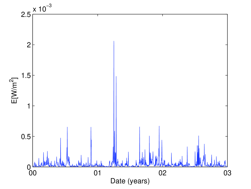
Figure 2: Energy-time series of solar flares from 2000 January 01 to 2002 December 31.

Now we restrict our attention to such time intervals, in which the solar activity is strong (in particular, 1978-1981, 1988-1992 and 1999-2003). We use X-ray flare data from GOES satellite, that contain information about time of appearance and energy of solar flares (from http://www.ngdc.noaa.gov/stp/SOLAR/ftpsolar-flares.html). The captured energy was transmitted by X-rays emitted during blasts on a solar surface from 2000 January 1 to 2002 December 31. We aggregated the energy values on a daily basis. The time series is presented in Fig. 2.

The first estimation procedure of the self-similarity parameter $H$ (i. e. the Hurst exponent)is the so-called finite impulse response transformation (FIRT). The FIRT estimator involve an array of coefficients. The array is made out of finite impulse response coefficients. The estimator $H_{FIRT}$ is obtained by performing a log-linear regression on the coefficients and measuring the slope (Stoev et al.2002). It is important to note that the estimator $H_{FIRT}$ is unbiased for all $\alpha$ falling in the range $(0,2)$.

An alternative method of testing scaling and correlation properties of a time series is the variance of residuals method (VR) (Peng et al. 1994). First, the series is divided into blocks of size $m$. Then, within each block, the partial sums of the series are calculated. A least -squares line is fitted to the partial sums within each block, and the sample variance of the residuals is computed. The variance of residuals is proportional to $m^{2H}$. This variance of residuals is computed for each block, and the median (or average) is computed over the blocks. A log -log plot versus $m$ should follow a straight line with a slope of $2H$.

The R/S method is one of the oldest and better known methods for estimation of the Hurst parameter (Hurst1951). Hurst found that drought in the Nile Valley is not a random phenomenon, but rather that the region is inclined to become progressively more arid after a succession of long droughts. It is widely known that for Gaussian (i.e. finite variance) time series the method returns $H$ (Mandelbrot & Wallis1969). The popularity of the method has been also a source of misunderstandings and errors. This is due to the fact that, in general, for power-law distributed time series (i.e. with infinite variance) the method yields $d+1/2$. In particular for Pareto or Lévy stable distributions the output is $H-1/\alpha+1/2$ (Taqqu & Teverovsky1998). The method is based on R/S (rescaled adjusted range) statistics. The series is divided into blocks. Then, within each block, the statistics is calculated. Finally, arithmetic means of the values of the statistics over the blocks are calculated and a least squares line is fitted to the mean for different lengths of the blocks. The slope should be equal to $d+1/2$.

For the finite variance cases, the interpretation of the FIRT and VR estimators is very similar to the Hurst exponent: if only short-range correlations (or no correlations at all) exist in the studied series, then $H_{FIRT}=H_{VR}=1/2$; if there is a correlation then $H_{FIRT}=H_{VR}\neq 1/2$. Moreover, if the estimator $H_{FIRT}=H_{VR}$ is greater than $1/2$, the time series is persistent and if $H_{FIRT}=H_{VR}<1/2$, then the time series is not persistent.

Note that both estimators give an information on memory and not on distribution of the process increments.

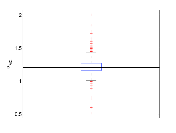
Figure 3: Values of the calculated $\alpha$ estimators for the simulated FARIMA time series. Solid line represents the value of the estimator for the analyzed data.

The analysis of the data shows that the tails of the underlying distribution conform to the power law. Hence, we model the data by a FARIMA process with Pareto innovations. As the power-law distributions belong to the domain of attraction of stable law (see, eg. Janicki & Weron1994) the resulting distribution of the FARIMA process should be close to the stable one. We applied the McCulloch quantile fit to obtain the parameters of the distribution (McCulloch1986). The value of $\alpha$ was estimated to be $1.213$, see Figure 3. One may check that the estimated value of $\alpha$ of simulated FARIMA times series with Pareto innovations is usually underestimated, see e. g. Figure 3. Therefore, we assume that the innovations in our model follow the Pareto law with $\alpha=1.25$.

According to Weron et al. (2005), in order to recover both the self-similarity exponent $H$ and the memory parameter $d$ (hence, the distribution parameter $\alpha$) we can use the following BMW² computer test. The surrogate data are obtained here by a random shuffling of the original data positions.

• If the process is FARIMA with Gaussian noise, then the values of the estimator should change to $1/2$ for the surrogate data independently on the initial values.

• If the process is FARIMA with $\alpha$-stable or Pareto noise for $\alpha<2$, then the values of the estimator should change to $1/\alpha$ for the surrogate data independently on the initial values.

The above formalism can be easily applied to determine basic features of an empirical data series. Now we employ this to study an empirical time series recorded from the system describing the energy of solar flares (Fig. 2). The obtained values of the parameters are listed in Table 1. Therefore, from the results for the surrogate data, the corresponding estimates for the parameter $1/\alpha$ are: $1/\alpha_{FIRT}=H_{FIRT}=0.8452$ and $1/\alpha_{VR}=H_{VR}=0.7722$. We observe that the estimators are close to the one assumed in our model: $1/\alpha_{MC}=0.8$. Moreover, we choose $d=0.19$ as the highest admissible value of $d$, which is close to the one obtained via the R/S method for the original data, see Table 1.

One may notice that the estimators of $H$ obtained via FIRT and VR methods, see Table 1, are greater than theoretically admissible in the FARIMA model, i. e. they exceed one. As stated in Burnecki et al. (2008), this can be justified by performing simulations of the FARIMA processes and estimating the parameter $H$ on the simulated time series via different methods. It appears that a reasonable percentage of the values of $H$ is higher than the data estimates, so one can not reject the hypothesis that the underlying model is the FARIMA(0,$d$,0) process. Nevertheless, we now look for an enhanced model which would describe better the behavior of different estimators obtained for the original and shuffled data, and would improve the fit in terms of the prediction error. Thus, we propose a slight generalization of the model incorporating the short-dependence component, namely FARIMA (2,$d$,0) model. We estimated the AR(2) coefficients: $a_{1}$ (linear term) and $a_{2}$ (quadratic term) via the mean-square error (MSE) minimalization scheme taking into account three statistics: FIRT, VR and RS, see Figure 4. The estimated values are: $a_{1}=0.02$ and $a_{2}=0.03$. The FARIMA processes were generated according to the algorithm presented by Stoev & Taqqu(2004).

We calculate $H_{FIRT}$, $H_{V}R$ and $d_{RS}$ estimators for the simulated FARIMA (2,$d$,0) processes (top panel in Figs. 5 and 6) and the corresponding shuffled data (bottom panel in Figs. 5 and 6). We generate $1000$ trajectories of size $2^{10}$ which is close to the length of the original solar data, i. e. 1089 and present the results in form of the so-called box plots. The box plot has lines at the lower quartile, median, and upper quartile values. The whiskers are lines extending from each end of the box to show the extent of the rest of the data. Outliers are data with values beyond the ends of the whiskers. If there is no data outside the whisker, a dot is placed at the bottom whisker. The results correspond to the analysis of the original solar data included in Table 1. Thus, our FARIMA simulations reconstruct well the structure of the original solar flares data.

We conclude that the proper model could be based on the FARIMA(2,$d$,0) process with Pareto innovations with the parameters $a_{1}=0.02$, $a_{2}=0.03$, $d=0.19$, and $\alpha=1.25$ which has the long-range dependence property since $d>1-2/\alpha$ (Burnecki et al. 2008). The Pareto distribution is also convenient for the present analysis because it gives a description of positive random variables whereas the Lévy-stable one for $1<\alpha<2$ is related to both positive and negative random variables, but a time series of x-ray flare energy is quite positive by definition.

We also calculated the 1-day-ahead prediction for the FARIMA(2,$d$,0) time series (for the prediction discussion in the infinite variance FARIMA case see Kokoszka1995). The results are depicted in Figure 7.

7 Concluding Remarks and Discussion

In this paper we demonstrate how self-similar models driven by Lévy stable noise can be useful for modeling X-ray solar data. To be more precise we have suggested the FARIMA(2,$d$,0) model with $\alpha$-stable noise for predicting solar flare appearance in the period of a strong solar activity.

The procedure is illustrated in Section 6 for the captured energy transmitted by X-rays emitted during blasts on a solar surface from 2000 January 1 to 2002 December 31. Comparing the values of the different estimators for the original data series and for the surrogate data we estimated the components of the self-similarity index corresponding to the memory of the time series ($d$) and to the tail properties of the time series values distribution ($\alpha$), see Table 1. Thus, this allows in principle to build a proper physical model for analyzing the solar activity.

The analysis of soft X-ray emission observations shows that this series is enough complicated in nature. We have seen a strong dependence of statistics on solar cycling in the data. However, if one takes year intervals, then this cycle influence becomes not so strong. This allows one to reconstruct a statistical model for predicting the soft X-ray solar activity on the nearest solar cycle. The soft X-ray solar time series contains both long-range dependence and heavy-tailed effects. The first creates a random number of strong bursts on a background, and the second forms their persistence between each other. The most convenient model for their joint description is a FARIMA time series. In view of solar cycling the model permits one to predict a time series of soft X-ray solar flares, when the solar activity will be again near its maximum in 2010-2014 years. While we do not claim that this model provides the only possible explanation, it does provide a rigorous statistical picture of the expected observations of X -ray solar flares.

Figure 1: The evolution of the tail index $\alpha$ during the last solar cycles 1974-2006 (top picture) obtained via the max self-similarity method, the bottom picture shows Wolf numbers (characterizing solar activity) in this period.

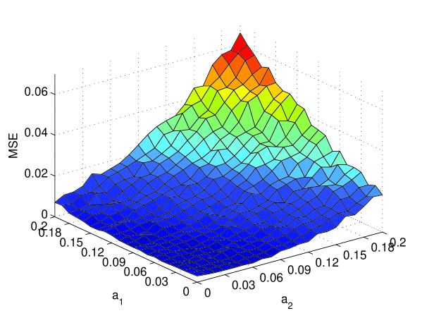
Figure 4: Mean squared error on the basis of the calculated $H$ and $d$ estimators for the simulated FARIMA time series with respects to the estimators obtained for the analyzed data for different $a_{1}$ and $a_{2}$.

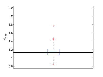
Figure 5: Values of the FIRT and VR estimators for the simulated time series (top panel) and the surrogate data (bottom panel) for the generated FARIMA processes. Solid line represents the value of the estimator for the analyzed data.

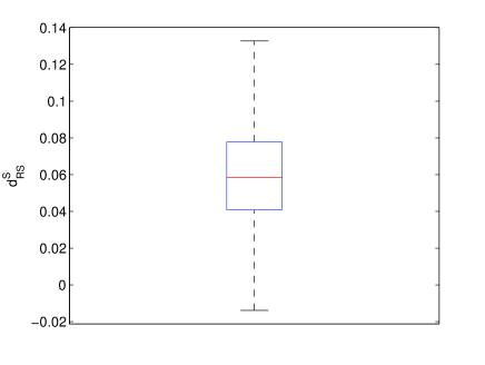
Figure 6: Values of the RS estimator $H_{RS}$ for the simulated time series (top panel) and the surrogate data (bottom panel) for the generated FARIMA processes. Solid line represents the value of the estimator for the analyzed data.

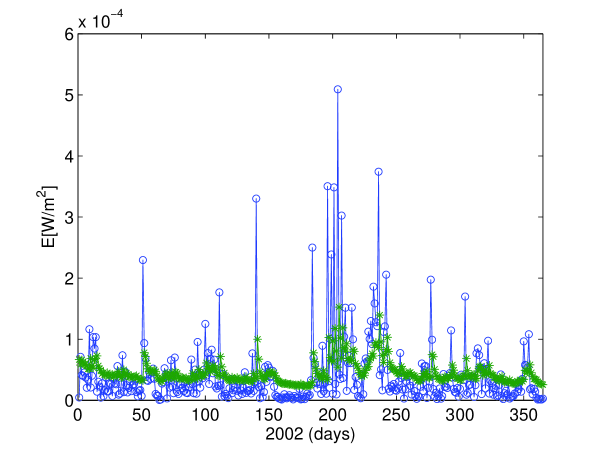
Figure 7: Solar flare data and prediction in the FARIMA(2,d,0) model.

Table 1: Values of the FIRT, VR and RS estimators for the original time series and the shuffled (surrogate) solar flare data.

Data set	$H_{FIRT}$	$H_{VR}$	$d_{RS}$
Original time series
Solar flares	$1.1424$	$1.0665$	$0.2408$
Surrogate data
Solar flares	$0.8452$	$0.7722$	$0.0507$

References

- Adler et al. (1998) Adler, R., Feldman R., & Taqqu, M.S. 1998, A Practical Guide to Heavy Tails: Statistical Techniques and Application (Boston: Birkhuser)
- Baiesi et al. (2006) Baiesi, M., Paczuski, M., & Stella, A.L. 2006, Phys. Rev. Lett., 96, 051103
- Beran (1994) Beran, J. 1994, Statistics for Long-Memory Processes (New York: Chapman & Hall)
- Boffetta et al. (1999) Boffetta, G., Carbone, V., Giuliani, P., Veltri, P., & Vulpiani, A. 1999, Phys. Rev. Lett., 83, 4662
- Burnecki et al. (2008) Burnecki, K., Klafter, J., Magdziarz M., & Weron, A. 2008, Physica A, 387, 1077
- Burnecki et al. (2005) Burnecki, K., Misiorek, A., & Weron, R., 2005, in Statistical Tools for Finance and Insurance, ed. P. Čížek, W. Hrdle, & R. Weron, (Berlin: Springer), 289
- Choudhuri et al. (2007) Choudhuri, A.R., Chatterjee, P., & Jiang, J. 2007, Phys. Rev. Lett., 98, 131103
- Clark (2006) Clark, S. 2006, Nature, 441, 402
- Dikrati & Gilman (2006) Dikpati, M., Gilman, P.A.: 2006, ApJ, 649, 498
- Dikpati et al. (2006) Dikpati, M., de Toma, G., & Gilman, P.A. 2006, Geophys. Res. Lett., 33, L05102
- Hurst (1951) Hurst, H.E. 1951, Transactions, American Society of Civil Engineers, 116, 770
- Kokoszka (1995) Kokoszka, P.S. 1995, Probab. Math. Statist., 16, 83
- Janicki & Weron (1994) Janicki, A., & Weron, A. 1994, A Simulation and Chaotic Behavior of -Stable Stochatic Processes (New York: Dekker)
- Lepreti et al. (2001) Lepreti, F., Carbone, C., & Veltri, P. 2001, ApJ, 555, L133
- Li et al. (1998) Li, K.-J., Schmieder, B., & Li, Q.-Sh. 1998, ApJS, 131, 99
- Lynch et al. (2005) Lynch, V.E., Carreras, B.A., Sanchez, R., LaBombard, B., van Milligen, B.Ph., & Newman D.E. 2005, Phys. Plasmas, 12, 052304
- Mandelbrot (1960) Mandelbrot, B.B. 1960, Int. Econ. Rev., 1, 79
- Mandelbrot & Wallis (1969) Mandelbrot, B.B. & Wallis, J. R. 1969, Water Resources Research, 5, 228
- Mann et al. (1998) Mann, M.E., Bradley, R.S., & Hughes, M.K. 1998, Nature, 392, 779
- McCulloch (1986) McCulloch, J.H. 1986, Comm. Statist. Simulation Comput., 15, 1109
- Moon et al. (2001) Moon, Y.-J., Choe, G.S., Yun, H.S., & Park, Y.D. 2001, J. Geophys. Res., 106, A12, 29951
- Nandy & Choudhuri (2002) Nandy, D., & Choudhuri, A. R. 2002, Science, 296, 1671
- Park & Willinger (2000) Park, K., & Willinger, W. 2000, Self-Similar Network Traffic and Performance Evaluation (New York: J. Wiley & Sons, Inc)
- Parker (1955) Parker, E.N. 1955, ApJ, 122, 293
- Peng et al. (1994) Peng, C.-K., Buldyrev, S. V., Havlin, S., Simons, M., Stanley, H. E., & Goldberger A. L. 1994, Phys. Rev. E, 49, 1685
- Samorodnitsky & Taqqu (1994) Samorodnitsky, G., & Taqqu, M. S. 1994, Stable NonGaussian Random Processes (New York: Chapman & Hall)
- Scafetta & West (2003) Scafetta, N., & West, B.J. 2003, Phys. Rev. Lett., 90, 248701
- Stoev et al. (2002) Stoev, S., Pipiras, V., & Taqqu M.S. 2002, Signal Processing, 82, 1873
- Stoev & Taqqu (2004) Stoev, S., & Taqqu, M. 2004, Fractals, 12, 1, 95
- Stoev & Michailidis (2006) Stoev, S., & Michailidis, G. 2006, Technical Report, 447, Department of Statistics, University of Michigan, http://www.stat.lsa.umich.edu/sstoev/max-spectrum-dep.pdf
- Svensmark & Friis-Christensen (1997) Svensmark, H., & Friis-Christensen, E. 1997, Solar -Terr. Phys., 59, 1225
- Taqqu & Teverovsky (1998) Taqqu, M.S., & Teverovsky, V. 1998, in A Practical Guide To Heavy Tails: Statistical Techniques and Applications, ed. R. Adler, R. Feldman & M. S. Taqqu (Boston: Birkhuser), 177
- Veronig et al. (2002) Veronig, A., Temmer, M., Hanslmeier, A., Otruba W., & Messerotti M. 2002, A&A, 382, 1078
- Weron (2001) Weron, R. 2001, Int. J. Mod. Phys. C, 12, 209
- Weron (2002) Weron, R. 2002, Physica A, 312, 285
- Weron et al. (2005) Weron, A., Burnecki, K., Mercik, Sz., & Weron, K. 2005, Phys. Rev. E, 71, 016113
- Wheatland (2002) Wheatland, M.S. 2002, Sol. Phys., 208, 33
- Zipf (1932) Zipf, G. 1932, Selective Studies and Principle of Relative Frequency in Language (Harvard University Press)