The Thermal Production of Strange and Non-Strange Hadrons in e+e- Collisions
Abstract
The thermal multihadron production observed in different high energy collisions poses two basic problems: (1) why do even elementary collisions with comparatively few secondaries (e+e- annihilation) show thermal behaviour, and (2) why is there in such interactions a suppression of strange particle production? We show that the recently proposed mechanism of thermal hadron production through Hawking-Unruh radiation can naturally account for both. The event horizon of colour confinement leads to thermal behaviour, but the resulting temperature depends on the strange quark content of the produced hadrons, causing a deviation from full equilibrium and hence a suppression of strange particle production. We apply the resulting formalism to multihadron production in annihilation over a wide energy range and make a comprehensive analysis of the data in the conventional statistical hadronization model and the modified Hawking-Unruh formulation. We show that this formulation provides a very good description of the measured hadronic abundances, fully determined in terms of the string tension and the bare strange quark mass; it contains no adjustable parameters.
I Introduction
Hadron production in high energy collisions shows remarkably universal thermal features. In annihilation Beca-e ; erice ; Beca-h , in , Beca-p and more general interactions Beca-h , as well as in the collisions of heavy nuclei Beca-hi , over an energy range from around 10 GeV up to the TeV range, the relative abundances of the produced hadrons appear to be those of an ideal hadronic resonance gas at a quite universal temperature MeV, as illustrated in Fig. 1 Beca-Biele . The transverse momentum spectra of the hadrons produced in hadronic collisions at intermediate energies are also in good agreement with the predictions of a statistical model based on the same temperature Beca-h .

There is, however, one important non-equilibrium effect observed: the production of strange hadrons in elementary collisions is suppressed relative to an overall equilibrium. This is usually taken into account phenomenologically by introducing an overall strangeness suppression factor Raf , which reduces the predicted abundances by and for hadrons containing one, two or three strange quarks (or antiquarks), respectively. In high energy heavy ion collisions, strangeness suppression becomes less and disappears at high energies gamma .
When comparing the temperatures of different collision channels in Fig. 1, it should be stressed that in elementary collisions, in contrast to heavy ion collisions, the conservation of charge, baryon number and strangeness is enforced exactly (canonical ensemble), so that here no chemical potential is introduced. The effect of exact charge conservation is important in elementary collisions because of the low multiplicities involved, while it is generally negligible in large multiplicity high energy nuclear reactions. The fitted values of lie around 0.5 to 0.7 in elementary collisions; the heavy ion values appear to vary as a function of energy, but it tend to approach unity gamma .
The origin of the observed thermal behaviour has been an enigma for many years and there is a still ongoing debate about the interpretation of these results diba . While the common belief is that in high energy heavy ion collisions multiple parton scattering could lead to kinetic thermalization through multiple scattering, or elementary hadron interactions do not readily allow such a description. The universality of the observed temperatures, on the other hand, suggests a common origin for all high energy collisions, and it was recently proposed CKS that thermal hadron production is the QCD counterpart of Hawking-Unruh radiation Hawk ; Un , emitted at the event horizon due to colour confinement. A well-known instance of this phenomenon is the Schwinger mechanism Schwinger ; KT of pair production in a constant electric field . The probability of spontaneously producing an electron-positron pair is in this case given by
| (1) |
where is the electron mass and its charge. Since
| (2) |
is just the acceleration of an electron (of reduced mass ) in the field , we find that the pair production probability has the thermal form
| (3) |
where
| (4) |
is the corresponding temperature. In other words, it is just that obtained by Unruh Un for the radiation emitted when a mass suffers constant acceleration and hence encounters an event horizon.
In the case of QCD and approximately massless quarks, the resulting hadronization temperature is determined by the string tension , with . The aim of the present work is to show that strangeness suppression occurs naturally in this framework, without requiring a specific suppression factor. The crucial role here is played by the non-negligible strange quark mass, which modifies the emission temperature for such quarks.
In this work, we will focus on e+e- collisions, which is the simplest case for this model to be tested. In the next section, we will briefly review the usual formulation of the statistical hadronization model, since this will form the basis also for the subsequent description in terms of Hawking-Unruh radiation model, to be formulated in Sect. 3. There we shall in particular derive the dependence of the radiation temperature on the mass of the produced quark and show how this affects the hadronization in annihilation. In Sect. 4, we then present an updated comprehensive analysis of all available data from GeV to GeV and compare the results of the Hawking-Unruh formulation to the conventional statistical description.
II Statistical Hadronization in Collisions
In this section we will briefly review the essentials of the statistical hadronization model and its application to e+e- collisions. For a detailed description see ref. meaning .
The statistical hadronization model assumes that hadronization in high energy collisions is a universal process proceeding through the formation of multiple colourless massive clusters (or fireballs) of finite spacial extension. These clusters are taken to decay into hadrons according to a purely statistical law: every multi-hadron state of the cluster phase space defined by its mass, volume and charges is equally probable. The mass distribution and the distribution of charges (electric, baryonic and strange) among the clusters and their (fluctuating) number are determined in the prior dynamical stage of the process. Once these distributions are known, each cluster can be hadronized on the basis of statistical equilibrium, leading to the calculation of averages in the microcanonical ensemble, enforcing the exact conservation of energy and charges of each cluster.
Hence, in principle, one would need the mentioned dynamical information in order to make definite quantitative predictions to be compared with data. Nevertheless, for Lorentz-invariant quantities such as multiplicities, one can introduce a simplifying assumption and thereby obtain a simple analytical expression in terms of a temperature. The key point is to assume that the distribution of masses and charges among clusters is again purely statistical Beca-h , so that, as far as the calculation of multiplicities is concerned, the set of clusters becomes equivalent, on average, to a large cluster (equivalent global cluster) whose volume is the sum of proper cluster volumes and whose charge is the sum of cluster charges (and thus the conserved charge of the initial colliding system). In such a global averaging process, the equivalent cluster generally turns out to be large enough in mass and volume so that the canonical ensemble becomes a good approximation of the more fundamental microcanonical ensemble Beca-micro ; in other words, a temperature can be introduced which replaces the a priori more fundamental description in terms of an energy density.
It should be stressed that in such an analysis of multiplicities, temperature has essentially a global meaning and not local as in hydrodynamical models. The only local meaningful quantity is cluster’s energy density, and even though the globally fitted temperature value is closely related to it, this does not mean that single physical clusters can be described in terms of a temperature, unless they are sufficiently large (about 10 GeV in mass, see Beca-micro ).
In the statistical hadronization model supplemented by global cluster averaging, the primary multiplicity of each hadron species is given by Beca-h
| (5) |
where is the (mean) volume and the temperature of the equivalent global cluster. Here is the canonical partition function depending on the initial abelian charges , i.e., electric charge, baryon number, strangeness, charm and beauty, respectively. We denote by and the mass and the spin of the hadron , and its corresponding charges; is the extra phenomenological factor implementing a suppression of hadrons containing strange valence quarks (see Sect. 1). In the sum (5), the upper sign applies to bosons and the lower sign to fermions. For temperature values of 160 MeV or higher, Boltzmann statistics corresponding to the term only in the series (5) is a very good approximation for all hadrons (within 1.5%) but pions. For resonances, the formula (5) is folded with a relativistic Breit-Wigner distribution of the mass .
The canonical partition function can be expressed as a multi-dimensional integral
| (6) |
where is the number of conserved abelian charges. Unlike the grand-canonical case, the logarithm of the canonical partition function does not scale linearly with the volume. Therefore, the chemical factors turn out to be less than unity at finite volume (canonical suppression) and only asymptotically reach their grand-canonical limit of unity, for an initially completely neutral system. Indeed, they play a major role in determining particle yields in e+e- collisions.
For all energies considered here, the production of heavy flavoured hadrons is negligible in events, where is a light quark (). As a result, in formula (5) the charm and bottom charge can be neglected, so that the abelian charge vector reduces to a three-component form and can be calculated with a numerical integration Beca-p ; chemfact . On the other hand, events, where is a heavy quark, always result in the production of two open heavy flavoured hadrons, arising from the primary heavy quark-antiquark pair, which subsequently decay into light-flavoured hadrons. In the statistical model, this constraint is readily implemented, requiring the number of heavy quarks plus antiquarks in the global description to be two; because of the high charm/bottom mass compared to the typical temperature value of 160 MeV, the probability of producing extra heavy pairs is absolutely negligible. The multiplicities of charm (bottom) hadrons in () events become in the Boltzmann approximation Beca-p ; erice
| (7) |
where
| (8) |
and denotes the canonical partition function as in (II), involving only light-flavoured particles, with . The indices label charm (bottom) hadrons, while the index their antiparticles.
The statistical treatment of heavy quark formation and hadronization as outlined here effectively means heavy quarks occur only in interactions, leading to one open charm (bottom) hadron and one corresponding antihadron per event. The relative rates of the different possible open charm (bottom) states, however, are determined by their phase space weights.
III String Breaking and Event Horizons
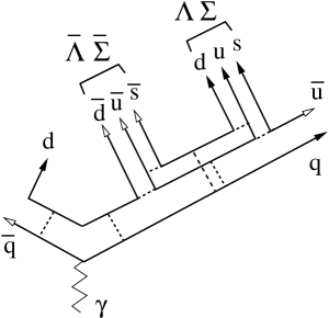
We first outline the thermal hadron production process through Hawking-Unruh radiation for the specific case of annihilation (see Fig. 2). The separating primary pair excites a further pair from the vacuum, and this pair is in turn pulled apart by the primary constituents. In the process, the shields the from its original partner , with a new string formed. When it is stretched to reach the pair production threshold, a further pair is formed, and so on bj ; nus . Such a pair production mechanism is a special case of Hawking-Unruh radiation KT , emitted as hadron when the quark tunnels through its event horizon to become .

The corresponding hadron radiation temperature is given by the Unruh form , where is the acceleration suffered by the quark due to the force of the string attaching it to the primary quark . This is equivalent to that suffered by quark due to the effective force of the primary antiquark . Hence we have
| (9) |
where is the effective mass of the produced quark, with for the bare quark mass and the quark momentum inside the hadronic system or . Since the string breaks CKS when it reaches a separation distance
| (10) |
the uncertainty relation gives us with
| (11) |
for the effective mass of the quark. The resulting quark-mass dependent Unruh temperature is thus given by
| (12) |
Note that here it is assumed that the quark masses for and are equal. For , eq. (12) reduces to
| (13) |
as obtained in CKS .
If the produced hadron consists of quarks of different masses, the resulting temperature has to be calculated as an average of the different accelerations involved. For one massless quark () and one of strange quark mass , the average acceleration becomes
| (14) |
From this the Unruh temperature of a strange meson is given by
| (15) |
with . Similarly, we obtain
| (16) |
for the temperature of a meson consisting of a strange quark-antiquark pair (). With GeV2, eq. (13) gives GeV. A strange quark mass of 0.1 GeV reduces this to GeV and MeV, i.e., by about 6 % and 12 %, respectively.
The scheme is readily generalized to baryons. The production pattern is illustrated in Fig. 3 and leads to an average of the accelerations of the quarks involved. We thus have
| (17) |
for nucleons,
| (18) |
for and production,
| (19) |
for production, and
| (20) |
for that of ’s. We thus obtain a resonance gas picture with five different hadronization temperatures, as specified by the strangeness content of the hadron in question: and .
![[Uncaptioned image]](/html/0805.0964/assets/x3.png)
It is important to stress that, in this picture, the primary quarks produced directly in the annihilation are not related to Hawking-Unruh radiation, nor are the light quarks with which they eventually combine to hadronize. Therefore, leading hadrons (those containing primary quarks) are essentially different and should be treated separately from hadrons containing only newly produced quarks. In practice, while in the conventional statistical model the same hadronization temperature governs the relative probabilities of emitting different species of leading hadrons, in the Hawking-Unruh formulation, we do not have any specific prescription for this. The problem of calculating leading hadron yields is relevant in e+e- annihilations because, in contrast to hadronic collisions, the primary heavy quarks and have large branching ratios and significantly contribute to the production of light-flavoured hadrons through the decay chain, especially in the strange sector. Lacking a definite recipe, we chose to calculate the relative heavy flavoured hadron yields by using the same temperatures as for light-flavoured ones, quoted above, keeping one weight fixed and using or according to whether the heavy quark hadronization occurs through combination with either or with , respectively. It should be noted out that this is not the only option and that different choices may lead to different results.
The different species-dependent temperatures are to be inserted into the formulae (5) and (7) of the previous section, in order to determine the primary hadron multiplicities. We note at this point a subtle conceptual difference between the conventional statistical approach and the Hawking-Unruh formulation. The usual statistical description employs, as noted above, a global cluster averaging, with each cluster statistically composed. In the Hawking-Unruh scheme, the radiation in each step is a hadron formed from the emitted pair, not some thermal cluster. Since the hadron can, however, be a highly excited resonance, the two descriptions become equivalent in a Hagedorn-type picture proposing resonances made up of resonances in a self-similar pattern.
The multiplicities obtained in the Hawking-Unruh scheme are, as emphasized, fully determined by the two basic parameters of the formulation, the string tension and the strange quark mass . Apart from possible variations of these quantities, our description is thus parameter-free. As illustration, we show in table 1 the temperatures obtained for GeV2 and three different strange quark masses. It is seen that in all cases, the temperature for a hadron carrying non-zero strangeness is lower than that of non-strange hadrons; as we shall show, this leads to an overall strangeness suppression.
| 0.178 | 0.178 | 0.178 | |
| 0.172 | 0.167 | 0.162 | |
| 0.166 | 0.157 | 0.148 | |
| 0.178 | 0.178 | 0.178 | |
| 0.174 | 0.171 | 0.167 | |
| 0.170 | 0.164 | 0.157 | |
| 0.166 | 0.157 | 0.148 |
Our picture implies that the produced hadrons are emitted slightly “out of equilibrium”, in the sense that the emission temperatures are not identical. As long as there is no final state interference between the produced quarks or hadrons, we expect to observe this difference and hence a modification of the production of strange hadrons, in comparison to the corresponding full equilibrium values. Once such interference becomes likely, as in high energy heavy ion collisions, equilibrium can be at least partially restored, weakening the strangeness suppression. The extension of our approach to heavy ion collisions will be dealt with in a subsequent paper.
IV Analysis of Hadron Multiplicities
Multihadron production in e+e- annihilation has been studied at PEP, PETRA and LEP over an energy range from 14 to 189 GeV, and the multiplicities of a large number of different species have been measured. The relevant data and their references are compiled in the Appendix.
In order to compare the models with the experimental data, we have at each energy made a fit to available measured multiplicities of light-flavoured hadrons, both in the traditional statistical model and in the Hawking-Unruh formulation. The traditional model has three free parameters to be determined, namely the temperature , the global volume (see the discussion in the Sect. 2), and the strangeness undersaturation parameter . In the Hawking-Unruh model, is kept, but the string tension and the strange mass replace and as fit parameters.
In the fit, the theoretical multiplicity of a given species, to be compared to the data, is calculated as the sum of primary multiplicity given by (5) and the contribution from the decay of unstable heavier hadrons,
| (21) |
where the branching ratios are the measured values as listed in the latest compilation of the Review of Particle Physics pdg . For the decays of heavy flavoured hadrons with unknown branching fractions, we have used the predictions of the PYTHIA pythia program. The hadrons considered unstable in e+e- experiments are all species except , , , , , and we have followed this convention in the theoretical calculation to meet the definition of measured multiplicities. The hadrons and resonances contributing to the sum in Eq. (21) consist here of all known states pdg up to a mass of 1.8 GeV.
A specific fraction of e+e- annihilations occurs into heavy and quarks. In this case, the multiplicities of light-flavoured hadrons are affected by the presence of the heavy quarks, both at primary level as the canonical partition function changes (see discussion in the previous section) and at final level because of the heavy flavoured hadron decays. This is taken into account in our calculations, and the production rate of the hadron is given by
| (22) |
where accounts for quarks and the index specifies the corresponding multiplicity in annihilation. The values of
| (23) |
are the corresponding branching fractions, obtained at each centre-of-mass energy from measurements and electroweak calculations. We have here taken the values calculated in the PYTHIA programme pythia , which are quoted in table 2 for each centre-of-mass energy.
| 14 | 0.46 | 0.09 | 0.37 | 0.08 |
|---|---|---|---|---|
| 22 | 0.46 | 0.09 | 0.36 | 0.09 |
| 29 | 0.46 | 0.09 | 0.36 | 0.09 |
| 35 | 0.46 | 0.09 | 0.36 | 0.09 |
| 43 | 0.46 | 0.09 | 0.36 | 0.09 |
| 91.25 | 0.39 | 0.22 | 0.17 | 0.22 |
| 133 | 0.41 | 0.18 | 0.23 | 0.18 |
| 161 | 0.42 | 0.17 | 0.24 | 0.17 |
| 183 | 0.42 | 0.16 | 0.26 | 0.16 |
| 189 | 0.42 | 0.16 | 0.26 | 0.16 |
The mass of resonances with MeV has been distributed according to a relativistic Breit-Wigner function over the interval , where is the central mass value and , being the width and the threshold mass value for the opening of all allowed decay channels. The primary production rate of neutral mesons such as , , , and others, which are a superposition of and , states, has been suppressed with according to the fraction of content. For this purpose we use the mixing formulas quoted in the Review of Particles Properties pdg with angles and for the system and for system, respectively, while for other nonets we used .
For each experiment, the most recent measurements have been considered. Multiple measurements from different experiments have been averaged according to the PDG method pdg , with error rescaling in case of discrepancy, that is a of the weighted average . The overall calculated yields are compared to the experimental measurements , and the total overall ,
| (24) |
where are the experimental errors, is minimized. The minimization is in fact carried out in two steps, in order to take into account the uncertainties on input parameters, such as hadron masses, widths and branching ratios, according to the following procedure Beca-h . First a with only experimental errors is minimised and preliminary best-fit model parameters are determined. Then, keeping the preliminarly fitted parameters fixed, the variations of the multiplicities corresponding to the variations of the input parameter by one standard deviation are calculated. Such variations are considered as additional systematic uncertainties on the multiplicities and the following covariance matrix is formed,
| (25) |
to be added to the experimental covariance matrix . Finally a new is minimised with covariance matrix , from which the best-fit estimates of the parameters and their errors are obtained. Actually, more than 350 among the most relevant or poorly known input parameters have been varied. However, it should be mentioned that no variation of the branching fractions of heavy flavoured hadrons has been done. Therefore, for some specific species, the systematic error could have been underestimated.
V Results
V.1 Light flavoured hadrons
We begin our analysis with the most extensive sample, the LEP data at 91.25 GeV. It comes from a compilation of results from the four different experimental groups (see references at the end of the Appendix), and it lists up to 30 different light flavoured species. However, for short-lived and hence broad resonances, the separation of resonance signal from background often becomes difficult, making the assessment of systematic errors problematic. Moreover, broad resonances yields are more sensitive to feeding from possibly unobserved heavier states or poorly known branching ratios. For this reason, we first consider, both for the conventional and for the Hawking-Unruh scenario, the analysis of the unproblematic (“golden”) species of widths less than 10 MeV; this still leaves 15 different hadronic states to be analysed, listed in tables 3 and 4.


As noted, the conventional statistical resonance gas approach is based on a universal temperature , a strangeness suppression factor , and a global volume . The fit of the long-lived species is shown in detail in table 3 and fig. 4 and the resulting fit parameters are
| (26) |
with a /dof = 39/12. The errors on the parameters are the fit errors rescaled by . Such a method pdg takes into account the additional uncertainty on the parameters if the fit leads to . This rescaling has been applied to all parameter errors quoted in this paper.
Next, we perform the corresponding hadron-resonance gas analysis in the Hawking-Unruh formulation, introducing different temperatures determined by the string tension and the strange quark mass . The results for long-lived species are shown in table 4 and fig. 4. The resulting fit parameters here are
| (27) |
with a /dof = 22/12, somewhat better than that of the corresponding conventional fit.
We now repeat both analyses using the entire 91.25 GeV data set, with the results shown in table XX and XXI of the Appendix. The resulting fit values (see tables 3 and 4) agree well within errors with those obtained from the “golden” data set at 91.25 GeV. As expected, because of the mentioned error sizes, the for the full 91.25 set is considerably worse.
| Experiment (E) | Model (M) | Residual | M - E/E [%] | |
|---|---|---|---|---|
| 9.61 0.29 | 9.89 | 0.97 | 2.95 | |
| 8.50 0.10 | 8.48 | -0.14 | -0.167 | |
| 1.127 0.026 | 1.074 | -2.0 | -4.69 | |
| 1.0376 0.0096 | 1.0342 | -0.35 | -0.327 | |
| 1.059 0.086 | 1.020 | -0.46 | -3.72 | |
| 1.024 0.059 | 0.993 | -0.52 | -2.99 | |
| 0.519 0.018 | 0.572 | 3.0 | 10.3 | |
| 0.166 0.047 | 0.106 | -1.3 | -36.4 | |
| 0.0977 0.0058 | 0.1163 | 3.2 | 19.0 | |
| 0.1943 0.0038 | 0.1846 | -2.5 | -4.98 | |
| 0.0535 0.0052 | 0.0429 | -2.0 | -19.9 | |
| 0.0389 0.0041 | 0.0435 | 1.1 | 11.8 | |
| 0.0410 0.0037 | 0.0391 | -0.51 | -4.58 | |
| 0.01319 0.00050 | 0.01256 | -1.3 | -4.81 | |
| 0.00062 0.00010 | 0.00089 | 2.7 | 43.7 |
| Experiment (E) | Model (M) | Residual | M - E/E [%] | |
|---|---|---|---|---|
| 9.61 0.29 | 9.73 | 0.41 | 1.25 | |
| 8.50 0.10 | 8.32 | -1.7 | -2.06 | |
| 1.127 0.026 | 1.106 | -0.80 | -1.85 | |
| 1.0376 0.0096 | 1.0656 | 2.9 | 2.69 | |
| 1.059 0.086 | 1.006 | -0.61 | -4.98 | |
| 1.024 0.059 | 0.967 | -0.97 | -5.58 | |
| 0.519 0.018 | 0.559 | 2.2 | 7.78 | |
| 0.166 0.047 | 0.093 | -1.6 | -43.8 | |
| 0.0977 0.0058 | 0.1057 | 1.4 | 8.11 | |
| 0.1943 0.0038 | 0.1892 | -1.3 | -2.63 | |
| 0.0535 0.0052 | 0.0438 | -1.9 | -18.2 | |
| 0.0389 0.0041 | 0.0444 | 1.4 | 14.2 | |
| 0.0410 0.0037 | 0.0401 | -0.25 | -2.22 | |
| 0.01319 0.00050 | 0.01265 | -1.1 | -4.11 | |
| 0.00062 0.00010 | 0.00077 | 1.5 | 23.5 |
Here a comment is in order. The simple formulae (5) and (7), in both models, rely on some side assumptions (e.g. the special distributions for cluster charge fluctuations needed for the introduction of the equivalent global cluster) that are not expected to be exactly fulfilled. Therefore, those formulae are to be taken as a zero-order approximation and not as a faithful representation of the real process. Deviations from the introduced assumption entail corrections to the formulae (5) and (7) which are nevertheless very difficult to estimate. The theoretical error involved in these formulae becomes important when the accuracy of measurements is comparable and, in this case, a bad is to be expected. This is probably the case at GeV, where the relative accuracy of measurements is of the order of few percent for many particles. In this case, the fit is a useful tool to determine the best parameters of the “simplified” theory but should be used very carefully as a measure of the fit quality. As has been mentioned, in order to take into account the uncertainty on parameters implied in fits with , parameter errors have been rescaled by if this is larger than 1, according to Particle Data Group procedure pdg .
For all the remaining energies we have also carried out the corresponding analyses; the results are listed in tables 5 and 6 for the model parameters, while the comparison between measured and calculated multiplicities are shown in tables X to XXXI of the Appendix.
| [MeV] | /dof | |||
|---|---|---|---|---|
| 14 | 172.1 5.2 | 8.3 1.0 | 0.772 0.094 | 0.9 / 3 |
| 22 | 178.7 3.7 | 8.70 0.94 | 0.76 0.10 | 0.7 / 3 |
| 29 | 164.0 5.4 | 15.0 2.4 | 0.683 0.075 | 33 / 13 |
| 35 | 163.3 3.2 | 15.0 1.4 | 0.730 0.045 | 8.2 / 7 |
| 43 | 169 10 | 13.5 3.2 | 0.741 0.074 | 2.9 / 3 |
| 91 | 161.9 4.1 | 25.8 3.4 | 0.638 0.039 | 215 / 27 |
| 91* | 164.6 3.0 | 23.3 2.2 | 0.648 0.026 | 39 / 12 |
| 133 | 167.1 7.5 | 26.0 4.6 | 0.671 0.074 | 0.1 / 2 |
| 161 | 153.4 6.5 | 37.2 5.9 | 0.72 0.12 | 0.03 / 1 |
| 183 | 161 13 | 35 11 | 0.446 0.098 | 5.0 / 2 |
| 189 | 159 12 | 36 10 | 0.54 0.11 | 7.5 / 2 |
| [GeV2] | [MeV] | /dof | ||
|---|---|---|---|---|
| 14 | 0.185 0.015 | 133 24 | 71 19 | 0.9 / 3 |
| 22 | 0.199 0.017 | 140 32 | 77 20 | 0.7 / 3 |
| 29 | 0.1673 0.0096 | 240 36 | 78 15 | 38 / 13 |
| 35 | 0.1675 0.0065 | 237 23 | 74.6 6.5 | 8.8 / 7 |
| 43 | 0.178 0.020 | 216 48 | 76 16 | 3.2 / 3 |
| 91 | 0.1625 0.0078 | 406 52 | 82.3 7.8 | 217 / 27 |
| 91* | 0.1683 0.0042 | 368 24 | 83.2 4.0 | 23 / 12 |
| 133 | 0.175 0.015 | 418 69 | 89 16 | 0.1 / 2 |
| 161 | 0.148 0.029 | 590 220 | 74 24 | 0.03 / 1 |
| 183 | 0.165 0.026 | 550 160 | 130 28 | 5.1 / 2 |
| 189 | 0.161 0.029 | 560 180 | 110 36 | 7.7 / 2 |
The parameters and are shown in figs. 5 and 6 respectively. It can be seen that they are remarkably constant throughout the examined energy range from to 189 GeV.


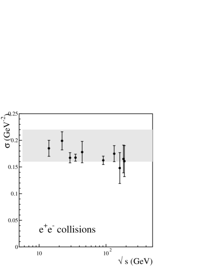
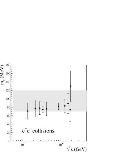
We now recall that the quantities we treated as fit parameters in the Hawking-Unruh analyses, the string tension and the strange quark mass, have in fact been determined in various other contexts and by different methods; they are quite well-known. The string tension is obtained in studies of heavy quarkonium spectroscopy as well as from Regge phenomenology. The canonical value JOS was GeV2; more recent calculations range from GeV2 Nora to 0.22 GeV2 BBC , giving an estimate of . The best average value of the strange quark mass is presently listed as pdg . In both cases we have good agreement with our fit values, as seen in fig. 6. We can thus indeed conclude that the Hawking-Unruh approach provides a parameter-free description of thermal hadron abundances in annihilation. The suppression of hadrons containing strange quarks is fully accounted for in terms of slight temperature changes due to the heavier strange quark mass. It is thus natural that this affects also non-strange hadrons dominantly made up of a strange quarks, such as the .
To illustrate the effect, we list in table 7 the different temperatures resulting from the different strange quark contents of the observed hadrons, using the fit parameters from the golden 91.25 data set. To check what such temperature differences can lead to, we compare the rate of direct production in the conventional to that of the Hawking-Unruh scenario. This direct rate is given by
| (28) |
in the conventional scenario; using the values (26) together with the production value listed in table 5, we obtain . Note that reduces the equilibrium value by more than a factor of two. The Hawking-Unruh scheme has with GeV a lower temperature for a meson containing a strange quark-antiquark pair than that governing light quark mesons. With
| (29) |
and the corresponding production volume of table 6, this leads to and hence practically the same value, however, without invoking the parameter . We note that these results should not be compared directly to the production measured in annihilation, which contains (at 91.25 GeV) a further 30 % due to feed-down contributions from charmed and bottomed hadron decay.
| [GeV] | |
|---|---|
| 0.164 | |
| 0.156 | |
| 0.148 | |
| 0.164 | |
| 0.158 | |
| 0.153 | |
| 0.148 |
V.2 Heavy flavoured hadrons
As has been mentioned in the previous section, the calculation of heavy flavoured hadron yields in and events is necessary to determine the final light flavoured hadron multiplicities. The heavy flavoured hadron relative abundances in such events are determined according to formula (7). For the conventional formulation of the statistical model, one has the same temperature as for the light-flavoured hadron species, while for the Hawking- Unruh radiation model, we do not have a definite prescription and we chose to use the same temperatures as for the light flavoured hadrons, which are dependent on the quark content.
Once the model parameters have been fitted by using light-flavoured hadronic multiplicities, they can be used to predict relative yields of heavy flavoured species in and annihilations and compare them to measured ones. This is a powerful, parameter-free, independent test of the conventional statistical model and a necessary consistency check for the Hawking-Unruh radiation model. Also, comparing theoretical values to measured relative abundances of heavy flavoured hadrons in specific annihilations channels (e.g. charmed hadrons in ) we achieve a more effective test because, e.g., the contribution of weak decays is excluded.
The relative yields of several heavy flavoured hadronic species have been measured in e+e- collisions at 91.25 GeV by the four LEP experiments. We show a comparison between model and weighted averaged experimental values in tables 8 and 9.
For the statistical model (table 8), the theoretical values have been estimated by using the parameters in eq. (26). The agreement between model and experiment is strikingly good, with few peculiar deviations in heavier states. In all those cases we observe an underestimation of measured values which may partly be explained by the absence, in our input spectrum, of unknown heavier heavy flavoured resonances feeding these states. It is quite remarkable that the model is able to reproduce the largely different ratios in the charm () and bottomed () sector - a long-standing issue in string models - without any additional parameter. This result confirms previous early findings Beca-e ; santorini .
| Particle | Experiment (E) | Model (M) | Residual | [%] | |
|---|---|---|---|---|---|
| 99bg | 0.559 0.022 | 0.5406 | -0.83 | -3.2 | |
| 99bg | 0.238 0.024 | 0.2235 | -0.60 | -6.1 | |
| 97ki ; 99bg ; 99vx | 0.2377 0.0098 | 0.2279 | -1.00 | -4.1 | |
| 98as | 0.218 0.071 | 0.2311 | 0.18 | 6.0 | |
| alconf ; 97vc | 0.0173 0.0039 | 0.01830 | 0.26 | 5.8 | |
| alconf ; 97vc | 0.0484 0.0080 | 0.02489 | -2.94 | -48.6 | |
| 99bg | 0.116 0.036 | 0.1162 | 0.006 | 0.19 | |
| 99bg | 0.069 0.026 | 0.0674 | -0.06 | -2.4 | |
| 01nj ; 97vc | 0.0106 0.0025 | 0.00575 | -1.94 | -45.7 | |
| 01nj | 0.0140 0.0062 | 0.00778 | -1.00 | -44.5 | |
| 99bg | 0.079 0.022 | 0.0966 | 0.80 | 22.2 | |
| Abbaneo:2001bv | 0.399 0.011 | 0.3971 | -0.18 | -0.49 | |
| Abbaneo:2001bv | 0.098 0.012 | 0.1084 | 0.87 | 10.6 | |
| (uds) | 96gz ; 95mt ; 95ky ; 94qv | 0.749 0.040 | 0.6943 | -1.37 | -7.3 |
| 98cq ; delconf ; 94fz | 0.180 0.025 | 0.1319 | -1.92 | -26.7 | |
| delconf | 0.090 0.018 | 0.0800 | -0.57 | -11.4 | |
| delconf | 0.0093 0.0024 | 0.00631 | -1.24 | -32.1 | |
| b-baryon | Abbaneo:2001bv | 0.103 0.018 | 0.09751 | -0.30 | -5.3 |
| Abbaneo:2001bv | 0.011 0.006 | 0.00944 | -0.26 | -14.2 |
For the Hawking-Unruh radiation model (table 9), the agreement between theoretical multiplicities, calculated with the parameters in eq. (27) and experiment is generally good, although not as good as for the conventional scheme. In fact, there are some specific discrepancies, especially in the beauty sector. In particular, we underestimate the relative yield of mesons, which is an effect of the lower temperature for open strange particles combined with the high mass of these particles, compared to light-flavoured species. In general, the way heavy flavoured hadrons are to be calculated in this model is still an open issue.
| Particle | Experiment (E) | Model (M) | Residual | [%] | |
|---|---|---|---|---|---|
| 99bg | 0.559 0.022 | 0.5635 | 0.20 | 0.81 | |
| 99bg | 0.238 0.024 | 0.2332 | -0.20 | -2.0 | |
| 97ki ; 99bg ; 99vx | 0.2377 0.0098 | 0.2373 | -0.04 | -0.18 | |
| 98as | 0.218 0.071 | 0.2407 | 0.32 | 10.4 | |
| alconf ; 97vc | 0.0173 0.0039 | 0.01897 | 0.43 | 9.6 | |
| alconf ; 97vc | 0.0484 0.0080 | 0.02577 | -2.82 | -46.8 | |
| 99bg | 0.116 0.036 | 0.08460 | -0.87 | -27.1 | |
| 99bg | 0.069 0.026 | 0.04793 | -0.81 | -30.5 | |
| 01nj ; 97vc | 0.0106 0.0025 | 0.00356 | -2.82 | -66.5 | |
| 01nj | 0.0140 0.0062 | 0.00479 | -1.49 | -66.1 | |
| 99bg | 0.079 0.022 | 0.09922 | 0.92 | 25.6 | |
| Abbaneo:2001bv | 0.399 0.011 | 0.4390 | 3.64 | 10.0 | |
| Abbaneo:2001bv | 0.098 0.012 | 0.0276 | -5.87 | -71.9 | |
| (uds) | 96gz ; 95mt ; 95ky ; 94qv | 0.749 0.040 | 0.6978 | -1.28 | -6.8 |
| 98cq ; delconf ; 94fz | 0.180 0.025 | 0.1479 | -1.28 | -17.8 | |
| delconf | 0.090 0.018 | 0.0894 | -0.04 | -0.72 | |
| delconf | 0.0093 0.0024 | 0.00136 | -3.31 | -85.3 | |
| b-baryon | Abbaneo:2001bv | 0.103 0.018 | 0.0944 | -0.48 | -8.4 |
| Abbaneo:2001bv | 0.011 0.006 | 0.00415 | -1.14 | -62.2 |
VI Conclusions
We have shown that in accord with previous studies Beca-e ; erice ; Beca-h , the thermal hadron abundances observed in e+e- collisions over a wide range of energies can indeed be accounted for in an ideal resonance gas scenario, based on a universal temperature MeV and a strangeness suppression factor . The latter is the ad hoc price paid in order to account for the deviation from full chemical equilibrium observed in the data. Remarkably, also the relative abundances of heavy flavoured species are in very good agreement with the statistical-thermal ansatz.
The Hawking-Unruh scenario, on the other hand, provides an intrinsic deviation from full equilibrium through the dependence of the radiation temperature on the mass of the emitted quark. Given the value of this mass and the string tension specifying the field strength at the confinement horizon, we then have a parameter-free prediction of the relative hadron abundances. We have seen here that these predictions agree well with the data at all energies, with the caveat that the relative multiplicities of heavy flavoured hadron species are not completely understood in this picture and are in slightly worse agreement with respect to the conventional statistical model. In a subsequent paper, we shall extend the Hawking-Unruh description to high energy heavy ion collisions, where it becomes significantly modified.
In closing, we comment on the degree of agreement between experiment and theory in our description. Hawking-Unruh radiation is thermal in leading order P-W , with higher order interaction terms. Similarly, one expects corrections to the simplest statistical hadronization model formulae, see discussion in Sect. 4. When accuracy of measurements is good enough, such higher-order effects must be taken into account and the fit quality to the simplest formulae unavoidably degrades. It is an interesting question to see if nuclear collisions, with a higher degree of averaging, lead to smaller deviations with measurements of the same accuracy.
Note added in proof
After completion of this work, another analysis of hadron production in annihilation has appeared, reaching very different conclusions pbmee . However, in contrast to our work, it is assumed in that analysis that the conservation of charm and bottom can be neglected. In annihilation, more than 40% of all events contain a primary charm or bottom quark-antiquark pair (see our table 2), hence two heavy-flavoured hadrons. Neglecting the corresponding conservation conditions and the decay contributions of these heavy-flavoured hadrons into light-flavoured hadrons necessarily produces serious disagreement with the data, especially for strange particles.
Appendix
In the following Tables 10 - 29, the experimental data and the statistical hadronization model predictions for various hadron multiplicities are compared. The first column shows the experimental value while in the second column, the statistical hadronization model prediction is quoted. In the fourth column one can find the relative deviation of the model from the experiment in percentage while the third column shows the residuals defined as
| (30) |
in which and are the theoretical and experimental multiplicitites and is the (experimental) standard error of a particle species . For each of the energies, we show 2 different tables one after the other so that always the first table shows the conventional statistical hadronization model fit results while the following one shows the same information in the Hawking-Unruh approach.
| Experiment (E) | Model (M) | Residual | (M - E)/E (%) | ||
|---|---|---|---|---|---|
| Bartel:1985wn | 4.69 0.20 | 4.65 | -0.18 | -0.752 | |
| Althoff:1984iz | 3.60 0.30 | 3.79 | 0.62 | 5.18 | |
| Althoff:1984iz | 0.600 0.070 | 0.589 | -0.15 | -1.81 | |
| Althoff:1984iz ; Bartel:1983qp | 0.563 0.045 | 0.556 | -0.15 | -1.17 | |
| Althoff:1984iz | 0.210 0.030 | 0.199 | -0.37 | -5.36 | |
| Althoff:1984iz | 0.065 0.020 | 0.077 | 0.58 | 17.8 |
| Experiment (E) | Model (M) | Residual | (M - E)/E (%) | ||
|---|---|---|---|---|---|
| Bartel:1985wn | 4.69 0.20 | 4.66 | -0.17 | -0.712 | |
| Althoff:1984iz | 3.60 0.30 | 3.79 | 0.62 | 5.16 | |
| Althoff:1984iz | 0.600 0.070 | 0.589 | -0.16 | -1.85 | |
| Althoff:1984iz ; Bartel:1983qp | 0.563 0.045 | 0.556 | -0.14 | -1.14 | |
| Althoff:1984iz | 0.210 0.030 | 0.198 | -0.39 | -5.52 | |
| Althoff:1984iz | 0.065 0.020 | 0.077 | 0.58 | 17.8 |
| Experiment (E) | Model (M) | Residual | (M - E)/E (%) | ||
|---|---|---|---|---|---|
| Bartel:1985wn | 5.50 0.40 | 5.49 | -0.033 | -0.238 | |
| Althoff:1984iz | 4.40 0.50 | 4.54 | 0.28 | 3.16 | |
| Althoff:1984iz | 0.75 0.10 | 0.69 | -0.65 | -8.64 | |
| Bartel:1983qp ; Braunschweig:1989wg | 0.638 0.057 | 0.651 | 0.22 | 1.96 | |
| Althoff:1984iz | 0.310 0.030 | 0.305 | -0.16 | -1.51 | |
| Althoff:1984iz | 0.110 0.025 | 0.117 | 0.29 | 6.70 |
| Experiment (E) | Model (M) | Residual | (M - E)/E (%) | ||
|---|---|---|---|---|---|
| Bartel:1985wn | 5.50 0.40 | 5.49 | -0.020 | -0.148 | |
| Althoff:1984iz | 4.40 0.50 | 4.54 | 0.28 | 3.18 | |
| Althoff:1984iz | 0.75 0.10 | 0.68 | -0.65 | -8.71 | |
| Bartel:1983qp ; Braunschweig:1989wg | 0.638 0.057 | 0.651 | 0.22 | 1.94 | |
| Althoff:1984iz | 0.310 0.030 | 0.305 | -0.17 | -1.65 | |
| Althoff:1984iz | 0.110 0.025 | 0.118 | 0.31 | 7.02 |
| Experiment (E) | Model (M) | Residual | (M - E)/E (%) | ||
|---|---|---|---|---|---|
| Aihara:1984mi | 5.30 0.70 | 6.48 | 1.7 | 22.2 | |
| Aihara:1986mv | 5.35 0.25 | 5.42 | 0.26 | 1.23 | |
| Aihara:1986mv | 0.700 0.050 | 0.747 | 0.93 | 6.66 | |
| Schellman:1984yz ; Aihara:1984mk ; Abachi:1989pr | 0.691 0.029 | 0.712 | 0.73 | 3.05 | |
| Abachi:1987qd ; Wormser:1988ru | 0.584 0.075 | 0.654 | 0.92 | 11.8 | |
| Abachi:1989em | 0.900 0.050 | 0.745 | -3.1 | -17.2 | |
| Abachi:1987wc | 0.310 0.030 | 0.237 | -2.4 | -23.7 | |
| Abachi:1989em ; Aihara:1984mk | 0.281 0.022 | 0.232 | -2.2 | -17.3 | |
| Aihara:1986mv | 0.300 0.050 | 0.300 | 0.0038 | 0.0627 | |
| Wormser:1988ru | 0.26 0.10 | 0.07 | -1.8 | -71.6 | |
| Aihara:1984pw | 0.084 0.022 | 0.092 | 0.35 | 9.15 | |
| Aihara:1984wx ; delaVaissiere:1984xg ; Geld:1992si | 0.0983 0.0060 | 0.1016 | 0.56 | 3.43 | |
| Klein:1986ws ; Abachi:1987ac | 0.0083 0.0020 | 0.0070 | -0.64 | -15.4 | |
| Abachi:1987ac | 0.0083 0.0024 | 0.0111 | 1.2 | 34.2 | |
| Abachi:1987wc | 0.045 0.022 | 0.016 | -1.3 | -64.4 | |
| Klein:1987fu | 0.0070 0.0036 | 0.0005 | -1.8 | -93.4 |
| Experiment (E) | Model (M) | Residual | (M - E)/E (%) | ||
|---|---|---|---|---|---|
| Aihara:1984mi | 5.30 0.70 | 6.37 | 1.5 | 20.2 | |
| Aihara:1986mv | 5.35 0.25 | 5.31 | -0.15 | -0.715 | |
| Aihara:1986mv | 0.700 0.050 | 0.760 | 1.2 | 8.55 | |
| Schellman:1984yz ; Aihara:1984mk ; Abachi:1989pr | 0.691 0.029 | 0.725 | 1.2 | 4.96 | |
| Abachi:1987qd ; Wormser:1988ru | 0.584 0.075 | 0.643 | 0.78 | 10.0 | |
| Abachi:1989em | 0.900 0.050 | 0.727 | -3.5 | -19.2 | |
| Abachi:1987wc | 0.310 0.030 | 0.231 | -2.6 | -25.6 | |
| Abachi:1989em ; Aihara:1984mk | 0.281 0.022 | 0.227 | -2.4 | -19.3 | |
| Aihara:1986mv | 0.300 0.050 | 0.292 | -0.17 | -2.82 | |
| Wormser:1988ru | 0.26 0.10 | 0.07 | -1.9 | -75.0 | |
| Aihara:1984pw | 0.084 0.022 | 0.084 | -0.022 | -0.593 | |
| Aihara:1984wx ; delaVaissiere:1984xg ; Geld:1992si | 0.0983 0.0060 | 0.1024 | 0.69 | 4.24 | |
| Klein:1986ws ; Abachi:1987ac | 0.0083 0.0020 | 0.0068 | -0.72 | -17.5 | |
| Abachi:1987ac | 0.0083 0.0024 | 0.0111 | 1.2 | 34.8 | |
| Abachi:1987wc | 0.045 0.022 | 0.014 | -1.4 | -69.9 | |
| Klein:1987fu | 0.0070 0.0036 | 0.0004 | -1.8 | -94.6 |
| Experiment (E) | Model (M) | Residual | (M - E)/E (%) | ||
|---|---|---|---|---|---|
| Braunschweig:1986hr ; Pitzl:1989qy ; Behrend:1989gn | 6.31 0.35 | 6.48 | 0.49 | 2.73 | |
| Braunschweig:1988hv | 5.45 0.25 | 5.42 | -0.14 | -0.621 | |
| Braunschweig:1988hv | 0.88 0.10 | 0.78 | -0.98 | -11.2 | |
| Bartel:1983qp ; Braunschweig:1989wg ; Behrend:1989ae | 0.740 0.017 | 0.746 | 0.33 | 0.759 | |
| Pitzl:1989qy ; Behrend:1989gn | 0.636 0.080 | 0.661 | 0.32 | 4.06 | |
| Althoff:1984iz ; Bartel:1984rh | 0.756 0.077 | 0.739 | -0.23 | -2.30 | |
| Bartel:1984rh ; Behrend:1989ae ; Braunschweig:1989wg | 0.361 0.046 | 0.248 | -2.4 | -31.2 | |
| Bartel:1981sw ; Braunschweig:1988hv | 0.302 0.033 | 0.300 | -0.078 | -0.838 | |
| Braunschweig:1988wh ; Behrend:1989ae | 0.108 0.010 | 0.108 | -0.042 | -0.391 | |
| Braunschweig:1988wh | 0.0060 0.0021 | 0.0079 | 0.90 | 31.5 |
| Experiment (E) | Model (M) | Residual | (M - E)/E (%) | ||
|---|---|---|---|---|---|
| Braunschweig:1986hr ; Pitzl:1989qy ; Behrend:1989gn | 6.31 0.35 | 6.46 | 0.41 | 2.31 | |
| Braunschweig:1988hv | 5.45 0.25 | 5.39 | -0.25 | -1.13 | |
| Braunschweig:1988hv | 0.88 0.10 | 0.78 | -0.97 | -11.0 | |
| Bartel:1983qp ; Braunschweig:1989wg ; Behrend:1989ae | 0.740 0.017 | 0.748 | 0.47 | 1.08 | |
| Pitzl:1989qy ; Behrend:1989gn | 0.636 0.080 | 0.657 | 0.26 | 3.33 | |
| Althoff:1984iz ; Bartel:1984rh | 0.756 0.077 | 0.735 | -0.28 | -2.82 | |
| Bartel:1984rh ; Behrend:1989ae ; Braunschweig:1989wg | 0.361 0.046 | 0.239 | -2.6 | -33.6 | |
| Bartel:1981sw ; Braunschweig:1988hv | 0.302 0.033 | 0.301 | -0.042 | -0.450 | |
| Braunschweig:1988wh ; Behrend:1989ae | 0.108 0.010 | 0.108 | 0.028 | 0.261 | |
| Braunschweig:1988wh | 0.0060 0.0021 | 0.0075 | 0.70 | 24.4 |
| Experiment (E) | Model (M) | Residual | (M - E)/E (%) | ||
|---|---|---|---|---|---|
| Braunschweig:1988hv ; Pitzl:1989qy | 6.66 0.65 | 6.63 | -0.055 | -0.541 | |
| Braunschweig:1988hv | 5.55 0.25 | 5.55 | -0.0021 | -0.00955 | |
| Braunschweig:1989bp | 0.96 0.15 | 0.81 | -1.0 | -15.9 | |
| Braunschweig:1989wg | 0.760 0.035 | 0.775 | 0.43 | 2.01 | |
| Braunschweig:1989wg | 0.385 0.094 | 0.264 | -1.3 | -31.3 | |
| Braunschweig:1988wh | 0.128 0.024 | 0.131 | 0.12 | 2.23 |
| Experiment (E) | Model (M) | Residual | (M - E)/E (%) | ||
|---|---|---|---|---|---|
| Braunschweig:1988hv ; Pitzl:1989qy | 6.66 0.65 | 6.62 | -0.065 | -0.639 | |
| Braunschweig:1988hv | 5.55 0.25 | 5.54 | -0.042 | -0.188 | |
| Braunschweig:1989bp | 0.96 0.15 | 0.81 | -1.0 | -15.8 | |
| Braunschweig:1989wg | 0.760 0.035 | 0.777 | 0.47 | 2.18 | |
| Braunschweig:1989wg | 0.385 0.094 | 0.255 | -1.4 | -33.6 | |
| Braunschweig:1988wh | 0.128 0.024 | 0.131 | 0.13 | 2.52 |
| Experiment (E) | Model (M) | Residual | (M - E)/E (%) | ||
|---|---|---|---|---|---|
| Acciarri:1994gza ; Adam:1995rf ; Barate:1996uh ; Abbiendi:2000cv | 9.61 0.29 | 10.20 | 2.0 | 6.18 | |
| Akers:1994ez ; Barate:1997ty ; Abreu:1998vq ; Abe:1998zs | 8.50 0.10 | 8.76 | 2.6 | 3.13 | |
| Akers:1994ez ; Barate:1997ty ; Abreu:1998vq ; Abe:1998zs | 1.127 0.026 | 1.091 | -1.4 | -3.20 | |
| Abreu:1994rg ; Acciarri:1994gza ; Abe:1998zs ; Abbiendi:2000cv ; Barate:1999gb | 1.0376 0.0096 | 1.0507 | 1.4 | 1.26 | |
| Acciarri:1994gza ; Abbiendi:2000cv ; Heister:2001kp | 1.059 0.086 | 1.041 | -0.21 | -1.70 | |
| Abreu:1998nn ; Krebs:1999iy | 1.40 0.13 | 1.19 | -1.6 | -15.0 | |
| Ackerstaff:1998ap | 1.20 0.22 | 1.14 | -0.26 | -4.66 | |
| Acciarri:1996tc ; Ackerstaff:1998ap ; Heister:2001kp | 1.024 0.059 | 1.014 | -0.17 | -0.997 | |
| Acton:1992us ; Abreu:1994rg ; Barate:1996fi | 0.357 0.022 | 0.353 | -0.16 | -1.02 | |
| Akers:1995wx ; Abreu:1996sn ; Barate:1996fi ; Abe:1998zs | 0.370 0.013 | 0.346 | -1.9 | -6.33 | |
| Akers:1994ez ; Abreu:1998vq ; Abe:1998zs ; Barate:1997ty | 0.519 0.018 | 0.564 | 2.5 | 8.76 | |
| Acciarri:1996tc ; Ackerstaff:1998ap | 0.166 0.047 | 0.106 | -1.3 | -36.1 | |
| Ackerstaff:1998ue ; Abreu:1998nn ; Krebs:1999iy | 0.1555 0.0085 | 0.0779 | -9.1 | -49.9 | |
| Ackerstaff:1998ap | 0.135 0.054 | 0.084 | -0.95 | -37.8 | |
| Abreu:1996sn ; Barate:1996fi ; Ackerstaff:1998ue ; Abe:1998zs | 0.0977 0.0058 | 0.1150 | 3.0 | 17.7 | |
| Abreu:1993mm ; Acciarri:1994gza ; Alexander:1996qj ; Abe:1998zs ; Barate:1999gb | 0.1943 0.0038 | 0.1779 | -4.3 | -8.42 | |
| Alexander:1996qi ; Acciarri:2000zf ; Abreu:1995qx | 0.0535 0.0052 | 0.0415 | -2.3 | -22.4 | |
| Alexander:1996qi ; Acciarri:2000zf ; Adam:1996hw ; Barate:1996fi | 0.0389 0.0041 | 0.0421 | 0.77 | 8.11 | |
| Alexander:1996qi ; Abreu:2000nu | 0.0410 0.0037 | 0.0378 | -0.85 | -7.65 | |
| Abreu:1995we ; Alexander:1995gq | 0.044 0.017 | 0.090 | 2.7 | 105. | |
| Ackerstaff:1998ue ; Abreu:1998nn ; Krebs:1999iy | 0.188 0.020 | 0.122 | -3.4 | -35.1 | |
| Abdallah:2003gu | 0.165 0.051 | 0.064 | -2.0 | -61.5 | |
| Abreu:1995qx ; Alexander:1996qj ; Barate:1996fi | 0.01319 0.00050 | 0.01187 | -2.6 | -10.0 | |
| Abreu:1995qx ; Alexander:1996qj ; Barate:1996fi | 0.0118 0.0011 | 0.0201 | 7.5 | 70.3 | |
| Abdallah:2003gu | 0.056 0.012 | 0.010 | -3.9 | -82.6 | |
| Abreu:1998nn | 0.036 0.012 | 0.026 | -0.91 | -29.2 | |
| Alexander:1996qj ; Abreu:2000nu | 0.0112 0.0014 | 0.0109 | -0.22 | -2.73 | |
| Abreu:1998nn | 0.0120 0.0058 | 0.0100 | -0.34 | -16.6 | |
| Abreu:1995qx ; Alexander:1996qj ; Barate:1996fi | 0.00289 0.00050 | 0.00417 | 2.6 | 44.4 | |
| Adam:1996hw ; Alexander:1996qj ; Barate:1996fi | 0.00062 0.00010 | 0.00081 | 1.9 | 31.0 |
| Experiment (E) | Model (M) | Residual | (M - E)/E (%) | ||
|---|---|---|---|---|---|
| Acciarri:1994gza ; Adam:1995rf ; Barate:1996uh ; Abbiendi:2000cv | 9.61 0.29 | 10.01 | 1.4 | 4.18 | |
| Akers:1994ez ; Barate:1997ty ; Abreu:1998vq ; Abe:1998zs | 8.50 0.10 | 8.57 | 0.77 | 0.918 | |
| Akers:1994ez ; Barate:1997ty ; Abreu:1998vq ; Abe:1998zs | 1.127 0.026 | 1.131 | 0.16 | 0.373 | |
| Abreu:1994rg ; Acciarri:1994gza ; Abe:1998zs ; Abbiendi:2000cv ; Barate:1999gb | 1.0376 0.0096 | 1.0901 | 5.5 | 5.05 | |
| Acciarri:1994gza ; Abbiendi:2000cv ; Heister:2001kp | 1.059 0.086 | 1.026 | -0.38 | -3.12 | |
| Abreu:1998nn ; Krebs:1999iy | 1.40 0.13 | 1.15 | -1.9 | -17.4 | |
| Ackerstaff:1998ap | 1.20 0.22 | 1.11 | -0.42 | -7.53 | |
| Acciarri:1996tc ; Ackerstaff:1998ap ; Heister:2001kp | 1.024 0.059 | 0.982 | -0.71 | -4.08 | |
| Acton:1992us ; Abreu:1994rg ; Barate:1996fi | 0.357 0.022 | 0.345 | -0.54 | -3.36 | |
| Akers:1995wx ; Abreu:1996sn ; Barate:1996fi ; Abe:1998zs | 0.370 0.013 | 0.338 | -2.5 | -8.62 | |
| Akers:1994ez ; Abreu:1998vq ; Abe:1998zs ; Barate:1997ty | 0.519 0.018 | 0.548 | 1.6 | 5.67 | |
| Acciarri:1996tc ; Ackerstaff:1998ap | 0.166 0.047 | 0.093 | -1.6 | -43.8 | |
| Ackerstaff:1998ue ; Abreu:1998nn ; Krebs:1999iy | 0.1555 0.0085 | 0.0751 | -9.5 | -51.7 | |
| Ackerstaff:1998ap | 0.135 0.054 | 0.081 | -1.0 | -40.0 | |
| Abreu:1996sn ; Barate:1996fi ; Ackerstaff:1998ue ; Abe:1998zs | 0.0977 0.0058 | 0.1048 | 1.2 | 7.19 | |
| Abreu:1993mm ; Acciarri:1994gza ; Alexander:1996qj ; Abe:1998zs ; Barate:1999gb | 0.1943 0.0038 | 0.1826 | -3.1 | -6.04 | |
| Alexander:1996qi ; Acciarri:2000zf ; Abreu:1995qx | 0.0535 0.0052 | 0.0424 | -2.1 | -20.7 | |
| Alexander:1996qi ; Acciarri:2000zf ; Adam:1996hw ; Barate:1996fi | 0.0389 0.0041 | 0.0430 | 1.00 | 10.5 | |
| Alexander:1996qi ; Abreu:2000nu | 0.0410 0.0037 | 0.0388 | -0.59 | -5.31 | |
| Abreu:1995we ; Alexander:1995gq | 0.044 0.017 | 0.086 | 2.5 | 95.0 | |
| Ackerstaff:1998ue ; Abreu:1998nn ; Krebs:1999iy | 0.188 0.020 | 0.115 | -3.7 | -38.9 | |
| Abdallah:2003gu | 0.165 0.051 | 0.061 | -2.0 | -63.2 | |
| Abreu:1995qx ; Alexander:1996qj ; Barate:1996fi | 0.01319 0.00050 | 0.01204 | -2.3 | -8.72 | |
| Abreu:1995qx ; Alexander:1996qj ; Barate:1996fi | 0.0118 0.0011 | 0.0204 | 7.8 | 72.8 | |
| Abdallah:2003gu | 0.056 0.012 | 0.007 | -4.1 | -87.3 | |
| Abreu:1998nn | 0.036 0.012 | 0.021 | -1.3 | -41.7 | |
| Alexander:1996qj ; Abreu:2000nu | 0.0112 0.0014 | 0.0106 | -0.45 | -5.55 | |
| Abreu:1998nn | 0.0120 0.0058 | 0.0068 | -0.89 | -43.1 | |
| Abreu:1995qx ; Alexander:1996qj ; Barate:1996fi | 0.00289 0.00050 | 0.00423 | 2.7 | 46.4 | |
| Adam:1996hw ; Alexander:1996qj ; Barate:1996fi | 0.00062 0.00010 | 0.00071 | 0.85 | 13.8 |
| Experiment (E) | Model (M) | Residual | (M - E)/E (%) | ||
|---|---|---|---|---|---|
| Abreu:2000gw | 9.92 0.26 | 9.94 | 0.063 | 0.167 | |
| Abreu:2000gw | 1.30 0.15 | 1.29 | -0.064 | -0.714 | |
| Abreu:2000gw | 1.25 0.12 | 1.25 | -0.070 | -0.663 | |
| Abreu:2000gw | 0.78 0.13 | 0.75 | -0.19 | -3.26 | |
| Abreu:2000gw | 0.250 0.038 | 0.256 | 0.15 | 2.27 |
| Experiment (E) | Model (M) | Residual | (M - E)/E (%) | ||
|---|---|---|---|---|---|
| Abreu:2000gw | 9.92 0.26 | 9.94 | 0.059 | 0.157 | |
| Abreu:2000gw | 1.30 0.15 | 1.29 | -0.060 | -0.669 | |
| Abreu:2000gw | 1.25 0.12 | 1.25 | -0.056 | -0.533 | |
| Abreu:2000gw | 0.78 0.13 | 0.76 | -0.17 | -2.92 | |
| Abreu:2000gw | 0.250 0.038 | 0.255 | 0.13 | 1.92 |
| Experiment (E) | Model (M) | Residual | (M - E)/E (%) | ||
|---|---|---|---|---|---|
| Abreu:2000gw | 10.38 0.38 | 10.37 | -0.00096 | -0.00355 | |
| Abreu:2000gw | 1.44 0.30 | 1.39 | -0.15 | -3.12 | |
| Abreu:2000gw | 1.32 0.18 | 1.34 | 0.094 | 1.31 | |
| Abreu:2000gw | 0.60 0.24 | 0.60 | -0.0010 | -0.0414 |
| Experiment (E) | Model (M) | Residual | (M - E)/E (%) | ||
|---|---|---|---|---|---|
| Abreu:2000gw | 10.38 0.38 | 10.37 | -0.0012 | -0.00431 | |
| Abreu:2000gw | 1.44 0.30 | 1.39 | -0.15 | -3.18 | |
| Abreu:2000gw | 1.32 0.18 | 1.34 | 0.097 | 1.34 | |
| Abreu:2000gw | 0.60 0.24 | 0.60 | -0.0011 | -0.0436 |
| Experiment (E) | Model (M) | Residual | (M - E)/E (%) | ||
|---|---|---|---|---|---|
| Abreu:2000gw | 10.89 0.29 | 10.87 | -0.081 | -0.216 | |
| Abreu:2000gw | 1.42 0.20 | 1.03 | -2.0 | -27.2 | |
| Abreu:2000gw | 0.905 0.086 | 0.995 | 1.0 | 9.97 | |
| Abreu:2000gw | 0.66 0.19 | 0.71 | 0.25 | 7.13 | |
| Abreu:2000gw | 0.165 0.025 | 0.161 | -0.15 | -2.35 |
| Experiment (E) | Model (M) | Residual | (M - E)/E (%) | ||
|---|---|---|---|---|---|
| Abreu:2000gw | 10.89 0.29 | 10.86 | -0.12 | -0.326 | |
| Abreu:2000gw | 1.42 0.20 | 1.03 | -1.9 | -27.0 | |
| Abreu:2000gw | 0.905 0.086 | 0.999 | 1.1 | 10.4 | |
| Abreu:2000gw | 0.66 0.19 | 0.73 | 0.36 | 10.5 | |
| Abreu:2000gw | 0.165 0.025 | 0.160 | -0.20 | -3.08 |
| Experiment (E) | Model (M) | Residual | (M - E)/E (%) | ||
|---|---|---|---|---|---|
| Abreu:2000gw | 11.10 0.26 | 11.06 | -0.15 | -0.344 | |
| Abreu:2000gw | 1.57 0.16 | 1.21 | -2.3 | -23.2 | |
| Abreu:2000gw | 1.060 0.078 | 1.169 | 1.4 | 10.3 | |
| Abreu:2000gw | 0.59 0.22 | 0.72 | 0.54 | 20.3 | |
| Abreu:2000gw | 0.200 0.021 | 0.196 | -0.20 | -2.16 |
| Experiment (E) | Model (M) | Residual | (M - E)/E (%) | ||
|---|---|---|---|---|---|
| Abreu:2000gw | 11.10 0.26 | 11.05 | -0.18 | -0.422 | |
| Abreu:2000gw | 1.57 0.16 | 1.21 | -2.3 | -23.2 | |
| Abreu:2000gw | 1.060 0.078 | 1.171 | 1.4 | 10.5 | |
| Abreu:2000gw | 0.59 0.22 | 0.74 | 0.64 | 23.7 | |
| Abreu:2000gw | 0.200 0.021 | 0.195 | -0.22 | -2.31 |
References
- (1) F. Becattini, Z. Phys. C69 (1996) 485.
- (2) F. Becattini, Universality of thermal hadron production in , and collisions, in Universality features in multihadron production and the leading effect, ,Singapore, World Scientific, 1998 p. 74-104, arXiv:hep-ph/9701275.
- (3) F. Becattini and G. Passaleva, Eur. Phys. J. C23 (2002) 551.
- (4) F. Becattini and U. Heinz, Z. Phys. C76 (1997) 268.
-
(5)
J. Cleymans et al., Phys. Lett. B 242 (1990) 111;
J. Cleymans and H. Satz, Z. Phys. C57 (1993) 135;
K. Redlich et al., Nucl. Phys. A 566 (1994) 391;
P. Braun-Munzinger et al., Phys. Lett. B344 (1995) 43;
F. Becattini, M. Gazdzicki and J. Sollfrank, Eur. Phys. J. C5 (1998) 143;
F. Becattini et al., Phys. Rev. C64 (2001) 024901;
P. Braun-Munzinger, K. Redlich and J. Stachel, in Quark-Gluon Plasma 3, R. C. Hwa and X.-N Wang (Eds.), World Scientific, Singapore 2003. - (6) F. Becattini, Nucl. Phys. A702 (2001) 336c.
- (7) J. Letessier, J. Rafelski and A. Tounsi, Phys. Rev. C64 (1994) 406.
- (8) See e.g. F. Becattini, J. Manninen and M. Gazdzicki, Phys. Rev. C 73 (2006) 044905; P. Braun-Munzinger, D. Magestro, K. Redlich and J. Stachel, Phys. Lett. B 518 (2001) 41.
-
(9)
U. Heinz, Nucl. Phys. A 661 (1999) 140;
R. Stock, Phys. Lett. B 456 (1999) 277;
A. Bialas, Phys. Lett. B 466 (1999) 301;
H. Satz, Nucl. Phys. Proc. Suppl. 94 (2001) 204;
J. Hormuzdiar,S. D. H. Hsu, G. Mahlon Int. J. Mod. Phys. E 12 (2003) 649; V. Koch, Nucl. Phys. A 715(2003) 108 ;
L. McLerran, arXiv:hep-ph/0311028;
Y. Dokshitzer, Acta Phys. Polon. B 36 (2005) 361;
F. Becattini, J. Phys. Conf. Ser. 5 (2005) 175. - (10) P. Castorina, D. Kharzeev and H. Satz, Eur. Phys. J. C52 (2007) 187.
- (11) S. W. Hawking, Comm. Math. Phys. 43 (1975) 199.
- (12) W. G. Unruh, Phys. Rev. D 14 (1976) 870.
- (13) J. Schwinger, Phys. Rev. 82 (1951) 664.
-
(14)
R. Brout, R. Parentani and Ph. Spindel, Nucl. Phys. B 353 (1991) 209;
P. Parentani and S. Massar, Phys. Rev. D 55 (1997) 3603;
K. Srinivasan and T. Padmanabhan, Phys. Rev. D60 (1999) 024007;
D. Kharzeev and K. Tuchin, Nucl. Phys. A 753, 316 (2005);
Sang Pyo Kim, arXiv:0709.4313 [hep-th] 2007 - (15) F. Becattini, J. Phys. Conf. Ser. 5 (2005) 175.
- (16) F. Becattini and L. Ferroni, Eur. Phys. J. C 35 (2004) 243; F. Becattini and L. Ferroni, Eur. Phys. J. C 38 (2004) 225.
- (17) A. Keranen and F. Becattini, Phys. Rev. C 65 (2002) 044901, Erratum-ibid. C 68 (2003) 059901.
- (18) J. D. Bjorken, Lecture Notes in Physics (Springer) 56 (1976) 93.
- (19) A. Casher, H. Neuberger and S. Nussinov, Phys. Rev. D20 (1979) 179.
- (20) W.-M. Yao et al. (2006 Review of Particle Physics), J. Phys. G 33 (2006) 1.
- (21) T. Sjostrand et al. Comp. Phys. Comm. 135 (2001) 238.
- (22) S. Jacobs, M. G. Olsson and C. Suchyta, Phys. Rev. D 33 (1986) 3338.
-
(23)
F. J. Yndurain, Theory of Quark and Gluon
Interactions, Springer Verlag Berlin, 1999;
N. Brambilla et al., CERN Yellow Report CERN-2005-005. -
(24)
C. Aubin et al. (MILC Collaboration), Phys. Rev. D70 (2004) 094505;
A. Gray et al., Phys. Rev. D72 (2005) 0894507,
M. Cheng et al., arXiv:hep-lat/0608013. - (25) F. Becattini, J. Phys. G 23 (1997) 1933.
- (26) M. K. Parikh and F. Wilczek, Phys. Rev. Lett. 85 (2000) 5042.
- (27) A. Andronic, F. Beutler, P. Braun-Munzinger, K. Redlich and J. Stachel, arXiv:0804.4132.
- (28) R. Barate et al. [ALEPH Collaboration], Eur. Phys. J. C 16 (2000) 597.
- (29) K. Ackerstaff et al. [OPAL Collaboration], Eur. Phys. J. C 1 (1998) 439.
- (30) P. Abreu et al. [DELPHI Collaboration], Eur. Phys. J. C 12 (2000) 209.
- (31) K. Ackerstaff et al. [OPAL Collaboration], Eur. Phys. J. C 5 (1998) 1.
- (32) TheALEPH Collaboration, “Production of D1 and D*2 mesons in hadronic Z decays”, preprint ALEPH 98-047 CONF 98-021 (1998).
- (33) K. Ackerstaff et al. [OPAL Collaboration], Z. Phys. C 76 (1997) 425.
- (34) A. Heister et al. [ALEPH Collaboration], Phys. Lett. B 526 (2002) 34.
- (35) The ALEPH, DELPHI, L3, OPAL and CDF Collaborations, “Combined results on b-hadron production rates and decay properties,” arXiv:hep-ex/0112028.
- (36) K. Ackerstaff et al. [OPAL Collaboration], Z. Phys. C 74 (1997) 413.
- (37) D. Buskulic et al. [ALEPH Collaboration], Z. Phys. C 69 (1996) 393.
- (38) P. Abreu et al. [DELPHI Collaboration], Z. Phys. C 68 (1995) 353.
- (39) M. Acciarri et al. [L3 Collaboration], Phys. Lett. B 345 (1995) 589.
- (40) R. Barate et al. [ALEPH Collaboration], Phys. Lett. B 425 (1998) 215.
- (41) Z. Albrecht et al. [DELPHI Collaboration] “A study of excited b-hadron states with the DELPHI detector at LEP”, preprint DELPHI-2004-025 CONF 700 (2004), presented at ICHEP 2004.
- (42) R. Akers et al. [OPAL Collaboration], Z. Phys. C 66 (1995) 19.
- (43) W. Bartel et al. [JADE Collaboration], Z. Phys. C 28 (1985) 343.
- (44) M. Althoff et al. [TASSO Collaboration], Z. Phys. C 27 (1985) 27.
- (45) W. Bartel et al. [JADE Collaboration], Z. Phys. C 20 (1983) 187.
- (46) W. Braunschweig et al. [TASSO Collaboration], Z. Phys. C 47 (1990) 167.
- (47) H. Aihara et al. [TPC/Two Gamma Collaboration], Z. Phys. C 27 (1985) 187.
- (48) H. Aihara et al. [TPC/Two Gamma Collaboration], Phys. Lett. B 184 (1987) 299.
- (49) H. Schellman et al., Phys. Rev. D 31 (1985) 3013.
- (50) H. Aihara et al. [TPC/Two Gamma Collaboration], Phys. Rev. Lett. 53 (1984) 2378.
- (51) S. Abachi et al. [HRS Collaboration], Phys. Rev. D 41 (1990) 2045.
- (52) S. Abachi et al. [HRS Collaboration], Phys. Lett. B 205 (1988) 111.
- (53) G. Wormser et al., Phys. Rev. Lett. 61 (1988) 1057.
- (54) S. Abachi et al., Phys. Rev. D 40 (1989) 706.
- (55) S. Abachi et al., Phys. Lett. B 199 (1987) 151.
- (56) H. Aihara et al. [TPC/Two Gamma Collaboration], Phys. Rev. Lett. 52 (1984) 2201.
- (57) H. Aihara et al. [TPC/Two Gamma Collaboration], Phys. Rev. Lett. 54 (1985) 274.
- (58) C. de la Vaissiere et al., Phys. Rev. Lett. 54 (1985) 2071 [Erratum-ibid. 55 (1985) 263].
- (59) T. L. Geld et al. [HRS Collaboration], Phys. Rev. D 45 (1992) 3949.
- (60) S. Klein et al., Phys. Rev. Lett. 58 (1987) 644.
- (61) S. Abachi et al., Phys. Rev. Lett. 58 (1987) 2627 [Erratum-ibid. 59 (1987) 2388].
- (62) S. Klein et al., Phys. Rev. Lett. 59 (1987) 2412.
- (63) W. Braunschweig et al. [TASSO Collaboration], Z. Phys. C 33 (1986) 13.
- (64) D. Pitzl et al. [JADE Collaboration], Z. Phys. C 46 (1990) 1 [Erratum-ibid. C 47 (1990) 676].
- (65) H. J. Behrend et al. [CELLO Collaboration], Z. Phys. C 47 (1990) 1.
- (66) W. Braunschweig et al. [TASSO Collaboration], Z. Phys. C 42 (1989) 189.
- (67) H. J. Behrend et al. [CELLO Collaboration], Z. Phys. C 46 (1990) 397.
- (68) W. Bartel et al. [JADE Collaboration], Phys. Lett. B 145 (1984) 441.
- (69) W. Bartel et al. [JADE Collaboration], Phys. Lett. B 104 (1981) 325.
- (70) W. Braunschweig et al. [TASSO Collaboration], Z. Phys. C 45 (1989) 209.
- (71) W. Braunschweig et al. [TASSO Collaboration], Z. Phys. C 45 (1989) 193.
- (72) M. Acciarri et al. [L3 Collaboration], Phys. Lett. B 328 (1994) 223.
- (73) W. Adam et al. [DELPHI Collaboration], Z. Phys. C 69 (1996) 561.
- (74) R. Barate et al. [ALEPH Collaboration], Z. Phys. C 74 (1997) 451.
- (75) G. Abbiendi et al. [OPAL Collaboration], Eur. Phys. J. C 17 (2000) 373.
- (76) R. Akers et al. [OPAL Collaboration], Z. Phys. C 63 (1994) 181.
- (77) R. Barate et al. [ALEPH Collaboration], Eur. Phys. J. C 5 (1998) 205.
- (78) P. Abreu et al. [DELPHI Collaboration], Eur. Phys. J. C 5 (1998) 585.
- (79) K. Abe et al. [SLD Collaboration], Phys. Rev. D 59 (1999) 052001.
- (80) P. Abreu et al. [DELPHI Collaboration], Z. Phys. C 65 (1995) 587.
- (81) R. Akers et al. [OPAL Collaboration], Z. Phys. C 67 (1995) 389.
- (82) R. Barate et al. [ALEPH Collaboration], Phys. Rept. 294 (1998) 1.
- (83) R. Barate et al. [ALEPH Collaboration], Eur. Phys. J. C 16 (2000) 613.
- (84) A. Heister et al. [ALEPH Collaboration], Phys. Lett. B 528 (2002) 19.
- (85) P. Abreu et al. [DELPHI Collaboration], Phys. Lett. B 449 (1999) 364.
- (86) W. Krebs [ALEPH Collaboration], ALEPH-99-057.
- (87) K. Ackerstaff et al. [OPAL Collaboration], Eur. Phys. J. C 5 (1998) 411.
- (88) M. Acciarri et al. [L3 Collaboration], Phys. Lett. B 393 (1997) 465.
- (89) P. D. Acton et al. [OPAL Collaboration], Phys. Lett. B 305 (1993) 407.
- (90) R. Akers et al. [OPAL Collaboration], Z. Phys. C 68 (1995) 1.
- (91) P. Abreu et al. [DELPHI Collaboration], Z. Phys. C 73 (1996) 61.
- (92) K. Ackerstaff et al. [OPAL Collaboration], Eur. Phys. J. C 4 (1998) 19.
- (93) P. Abreu et al. [DELPHI Collaboration], Phys. Lett. B 318 (1993) 249.
- (94) G. Alexander et al. [OPAL Collaboration], Z. Phys. C 73 (1997) 569.
- (95) P. Abreu et al. [DELPHI Collaboration], Z. Phys. C 67 (1995) 543.
- (96) G. Alexander et al. [OPAL Collaboration], Z. Phys. C 73 (1997) 587.
- (97) M. Acciarri et al. [L3 Collaboration], Phys. Lett. B 479 (2000) 79.
- (98) W. Adam et al. [DELPHI Collaboration], Z. Phys. C 70 (1996) 371.
- (99) P. Abreu et al. [DELPHI Collaboration], Phys. Lett. B 475 (2000) 429.
- (100) P. Abreu et al. [DELPHI Collaboration], Phys. Lett. B 361 (1995) 207.
- (101) G. Alexander et al. [OPAL Collaboration], Phys. Lett. B 358 (1995) 162.
- (102) J. Abdallah et al. [DELPHI Collaboration], Phys. Lett. B 569 (2003) 129.
- (103) P. Abreu et al. [DELPHI Collaboration], Eur. Phys. J. C 18 (2000) 203 [Erratum-ibid. C 25 (2002) 493].