We introduce stochastic Discrete Laplacian Growth and consider its deterministic continuous version. These are reminiscent respectively to well-known Diffusion Limited Aggregation and Hele-Shaw free boundary problem for the interface propagation. We study correlation between stability of deterministic free-boundary problem and macroscopic fractal growth in the corresponding discrete problem. It turns out that fractal growth in the discrete problem is not influenced by stability of its deterministic version. Using this fact one can easily provide a qualitative analytic description of the Discrete Laplacian Growth.

1 Introduction

The Laplacian Growth or zero surface tension Hele-Shaw free-boundary problem ( see e.g. [1], [6]) describes time evolution of a domain $\Omega=\Omega(t)$ in the complex plane with $z=x+iy$, when the boundary $\partial\Omega$ of the domain is driven by the gradient of a scalar field $\phi=\phi(x,y,t)$ (see Fig. 1). The field is harmonic, except for several singular points (”sources” and ”sinks”), in the exterior or the interior of $\Omega$. The corresponding Hele-Shaw problems are referred as exterior and interior respectively. The field $\phi$ vanishes at the domain boundary (”interface”) $\phi(\partial\Omega)=0$. Well possedness and stability of the problem depends strongly on types of singularities.

For instance, the exterior ”sink”-driven Hele-Shaw problem is a problem of expanding a simply-connected domain $\Omega$ whose boundary is driven by the field harmonic in exterior of $\Omega$. It is ill-posed and linearly unstable almost for any initial conditions. On the contrary, the exterior problem for contracting $\Omega$ (which is a ”source”-driven time reversal of the above problem) is linearly stable and well posed.

A discrete, stochastic version of the exterior Hele-Shaw problem (often called Diffusion Limited Aggregation or DLA, [2],[3],[7]) describes formation of a cluster of particles on two dimensional (e.g. square) lattice. No more than one particle can occupy a lattice cite. The particles stick one by one to the cluster. The probability for a particle to occupy a given (next to the cluster) cite is proportional to the value of a lattice harmonic field at that cite. The field has logarithmic ”sink”-type singularity at infinity. It vanishes on the cluster and is updated after each cluster increment.

The cluster in such a discrete problem is a fractal and one may think that instability and ill-possedness of the deterministic continuous version of such a discrete model (i.e. exterior Hele-Shaw free-boundary flow for expanding domain $\Omega$) is a manifestation of this fact. In other words, the fractal interface of the discrete problem may not be approximated by an analytic boundary curve of its deterministic counterpart.

In this article we consider a ”mix” of interior and exterior problems for simply-connected bounded domain, when the interface is driven by the scalar field $\phi$ which is harmonic almost everywhere except for the interface $\partial\Omega$ itself, where $\phi$ vanishes, and two logarithmic singular points. One of these points is placed at $z=0$ and other at $z=\infty$. In such systems the growth depends on a parameter $\lambda$ which is a measure of the ”mix” between the exterior unstable ($\lambda=0$) and the interior stable ($\lambda=1$) processes, with $\lambda=1/2$ being a ”neutral stability” growth.

One may expect that the fractal formations are not visible on macroscopic scale for discrete version of such models when $\lambda>1/2$ and when the interface is linearly stable. This turns out to be true only for extreme stability point $\lambda=1$, while the macroscopic fractal formations are present for any $\lambda<1$ in the discrete model.

Note that the Discrete Laplacian Growth (DLG) introduced here differs from the Diffusion Limited Aggregation (DLA) by simultaneous consideration of both exterior and interior processes on the lattice defined in a similar way. In the case of DLA one considers a lattice cluster and a complement to it, while in DLG the lattice is divided into interior domain, discrete boundary and exterior domain. Although the law of the cluster growth in pure exterior limit ($\lambda=0$) of DLG is locally different from that of DLA, both models have the same continuous version and belong essentially to the same class.

In the next section we describe, in details, the continuous version of the growth processes under consideration and perform its linear stability analysis.

2 Continuous Model

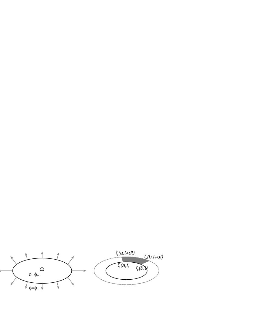
Figure 1: Problem setting (left) and the domain area increment along the boundary segment $a<l<b$ during the time interval $(t,t+dt)$ (right)

Let, for simplicity, $\Omega$ be a simply connected, bounded domain in the $z=x+iy$ plane with the point $z=0$ inside the domain. We denote by $\phi_{+}$ the field $\phi(x,y,t)$ in the interior and by $\phi_{-}$ in the exterior of the domain respectively (see Fig. 1). Field $\phi_{\pm}$ is harmonic in the interior/exterior of $\Omega$ except for points $z=0$ and $z=\infty$

$$\Delta\phi_{\pm}=0,\quad z\not\in\left\{0,\infty,\partial\Omega\right\}.$$ (1)

It is continuous across the boundary and vanishes on it

$$\phi_{\pm}(z\in\partial\Omega)=0$$ (2)

The field has logarithmic singularities at $z=0$ and $z=\infty$

$$\phi_{+}\to\frac{A_{+}}{2\pi}\log|z|,\quad z\to 0,\quad$$

$$\phi_{-}\to\frac{A_{-}}{2\pi}\log|z|,\quad z\to\infty$$

where $A_{\pm}$ are constants.

Consider the situation when the boundary dynamics is governed by gradients of $\phi_{\pm}$

$$v_{n}=\alpha_{+}\frac{\partial\phi_{+}}{\partial n}+\alpha_{-}\frac{\partial\phi_{-}}{\partial n},$$

where $\alpha_{\pm}$ are constants, $v_{n}$ denotes the normal velocity of the boundary

$$v_{n}={\rm Re}(nd\bar{z}/dt),\quad\bar{z}=x-iy,\quad z\in\partial\Omega,$$

$n=n_{x}+in_{y},|n|=1$ stands for the exterior normal to $\partial\Omega$ and $\partial/\partial n$ denotes the normal derivative at the boundary.

Rescaling the harmonic fields $\phi_{\pm}$ and the time variable $t$

$$\phi_{+}\to-\frac{A_{+}}{\lambda}\phi_{+},\quad\phi_{-}\to\frac{A_{-}}{1-\lambda}\phi_{-},\quad t\to\frac{\lambda}{\alpha_{+}A_{+}}t,\quad$$

where

$$\lambda=\frac{A_{+}\alpha_{+}}{A_{-}\alpha_{-}+A_{+}\alpha_{+}},$$

we rewrite the above dynamic law for the boundary velocity as

$$v_{n}=\frac{\partial\phi_{-}}{\partial n}-\frac{\partial\phi_{+}}{\partial n},$$ (3)

and field asymptotic now depend on a ”stability” parameter $\lambda$ as

$$\phi_{+}\to\frac{-\lambda}{2\pi}\log|z|,\quad z\to 0,\quad\phi_{-}\to\frac{1-\lambda}{2\pi}\log|z|,\quad z\to\infty.$$ (4)

Equations (1,2,3,4) together with the initial condition $\Omega(t=0)$ constitute a free-boundary, initial value problem for $\Omega(t)$.

Note, that the case $\lambda=0$ corresponds to the exterior Hele-Shaw problem (with $\phi_{+}=0$) while $\lambda=1$ refers to the interior Hele-Shaw problem (with $\phi_{-}=0$, respectively).

We are interested in discrete stochastic processes of lattice cluster growth, corresponding to the deterministic problem (1-4).

Consider first the case of cluster growing from a single particle at origin that corresponds to the circular solution of deterministic model. It is easy to see that such solution is an expanding circle of radius $r(t)=\sqrt{t/\pi}$ and $\phi_{\pm}=\phi^{(0)}_{\pm}$, where

$$\phi_{+}^{(0)}=\frac{-\lambda}{2\pi}(\log|z|-\frac{1}{2}\log\frac{t}{\pi}),\quad|z|<r(t),\quad$$

$$\phi^{(0)}_{-}=\frac{1-\lambda}{2\pi}(\log|z|-\frac{1}{2}\log\frac{t}{\pi}),\quad|z|>r(t)$$

Let us now study linear stability of this solution, considering small perturbations of the circle $|z|=r(t)$ by the $k$-periodic function

$$|z(\theta,t)|=r(t)+\epsilon r^{(k)}(t)\sin(k\theta)$$

where $\theta=(0,2\pi)$ is a polar angle on the $z$-plane ($z=|z|\exp(i\theta)$) and $k$ is a positive integer. The fields $\phi_{\pm}$ satisfying conditions (1), (4) are of the form

$$\phi_{\pm}=\phi_{\pm}^{(0)}+\epsilon\phi^{(k)}(t)|z/r(t)|^{\pm k}\sin(k\theta).$$

Substituting this and previous equations to (2) and (3) in the first order of $\epsilon$-series we get

$$\frac{dr^{(k)}}{dt}=\frac{1-2\lambda}{2t}kr^{(k)}$$ (5)

Since $k>0$, the perturbations grow in time when $\lambda<1/2$ and vanish in time when $\lambda>1/2$, with $\lambda=1/2$ being the ”neutral stability” point.

In this article we consider continuous systems labelled by stability parameter $\lambda$ in the range $0\leq\lambda\leq 1$. The $\lambda=0$ case (exterior Hele-Shaw problem for expanding interior domain) is unstable and ill-posed problem, whose discrete version manifests fractal growth. On the other extreme of the interval, at $\lambda=1$, we have stable and well-posed interior expansion problem.

Now it is natural to ask the question: Whether the stability of interior continuous problems (i.e. those at $\lambda>1/2$) may depress the macroscopic (i.e. visible in continuous limit) fractal growth of boundaries of corresponding discrete models?

To study this question, we are to introduce discrete analogue of the above problem (1-4).

3 Discrete Model

One may think of the free boundary problem (1-4) as that of dynamics of an ideal conducting contour $\partial\Omega$ in two-dimensional electric field. The field is created by a Coulomb charge of value $-\lambda$ at $z=0$ and unit charge distributed with linear density $\sigma(l,t)$ along the contour. The contour is ”an ideal conductor”, and this means that the potential (at fixed $t$) is constant along $\partial\Omega$. Here $l$ stands for natural parameter along the contour $\left\{\partial\Omega:z=\zeta(l,t),|d\zeta(l)|=dl\right\}$ and $\oint_{\partial\Omega}\sigma(l,t)dl=1$. The harmonic field $\phi(x,y,t)$ is (modulo coordinate independent function of $t$) the electrostatic potential created by the above charges

$$\phi=\frac{-\lambda}{2\pi}\log|z|+\frac{1}{2\pi}\oint_{\partial\Omega}\sigma(l,t)\log|z-\zeta(l,t)|dl$$

The gradient of the potential is the electric vector field, that has jump of magnitude $\sigma(l)$ across the boundary. Therefore from (3) it follows that the normal velocity of the contour equals its linear density

$$v_{n}(l,t)=\sigma(l,t)$$

This and the previous equations reduce the free-boundary problem on the plane to a dynamical problem on the contour only. It is easy to see that the density $\sigma$ is non-negative, and the interior domain $\Omega$ expands in time.

The domain area increment $dP_{(a,b)}$ along the interface segment $a<l<b$ during the time $dt$ (see Fig. 1)

$$\frac{dP_{(a,b)}}{dt}=\int_{a}^{b}v_{n}(l)dl=\int_{a}^{b}\sigma(l)dl=q_{(a,b)}$$ (6)

is proportional to the electric charge $q_{(a,b)}$ concentrated on this segment. This fact suggests to consider the boundary charge as the cluster increment probability in discrete analogue of the above model.

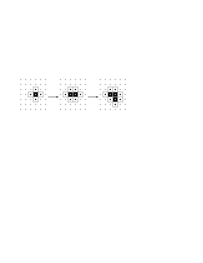
Figure 2: An example of the cluster growth. Black squares (”particles”) belong to the cluster $\Omega$, white squares with gray sides form the cluster boundary $\partial\Omega$. Black dots denote charged (boundary) cites and gray dots are uncharged lattice cites.

Let us now take a square lattice, paint elementary square cells in white color and label centers of squares by a pair of integers $(m,n)$ that are discrete coordinates along the $x$ and $y$ directions. Consider the following stochastic process: At the first step, the $(0,0)$ square is painted in black. At the next step we paint in black one of four cites that are next-neighbors of this smallest cluster e.t.c. (see Figure 2). This procedure is continued by coloring, at each step, any randomly chosen white next-neighbors of the cluster (i.e. adding randomly a ”particle” to the cluster) with the probability described below.

We use the same notation $\Omega$ for the cluster as we used for the continuous domain. The cluster boundary, which consists of all white next-neighbors of the cluster, is denoted, by analogy with continuous case, by $\partial\Omega$.

At each step of the process we can define a lattice function $\phi_{m,n}$ which satisfies the difference equation

$$\phi_{n-1,m}+\phi_{n+1,m}+\phi_{n,m-1}+\phi_{n,m+1}-4\phi_{n,m}=-\lambda\delta_{n,0}\delta_{m,0},\quad(n,m)\not\in\partial\Omega$$ (7)

everywhere except for the boundary, where it vanishes

$$\phi_{n,m}=0,\quad(n,m)\in\partial\Omega.$$ (8)

Its asymptotics is like follows

$$\phi_{n,m}\to\frac{1-\lambda}{4\pi}\log(m^{2}+n^{2}),\quad m^{2}+n^{2}\to\infty$$ (9)

The left hand side of (7) is a lattice Laplace operator, and $\delta$ on the right hand side stands for Kronecker delta symbol. Equations (7-9) are lattice analogues of (1, 2, 4).

As in the continuous case, the potential $\phi_{n,m}$ can be expressed in terms of charges, that are now placed at the boundary cites (see Fig. 2).

Introducing the lattice Coulomb potential (or the Green function) $G_{n,m}$, a such that

$$G_{n-1,m}+G_{n+1,m}+G_{n,m-1}+G_{n,m+1}-4G_{n,m}=\delta_{n,0}\delta_{m,0},\quad-\infty<n,m<\infty$$

and

$$G_{n,m}\to\frac{1}{4\pi}\log(m^{2}+n^{2}),\quad m^{2}+n^{2}\to\infty$$

one expresses $\phi_{n,m}$ in terms of $q_{i,j},(i,j)\in\partial\Omega$ as

$$\phi_{n,m}=\sum_{(i,j)\in\partial\Omega}q_{i,j}G_{n-i,m-j}-\lambda G_{n,m}+C$$

where $C$ is a constant.

It’s easy to see that the boundary charges are nonnegative $q_{i,j}\geq 0$. From (7), (9) and by the definition of the Green function it follows that

$$\sum_{(i,j)\in\partial\Omega}q_{i,j}=1.$$ (10)

By direct analogy with continuous case (c.f. (6)) we now consider $q_{i,j}$ as a probability of the $(i,j)$ square of the boundary $\partial\Omega$ to join the cluster $\Omega$.

Therefore, at each step of the growth process we have to solve the linear algebraic system consisting of equation (10) and

$$\sum_{(i^{\prime},j^{\prime})\in\partial\Omega}q_{i^{\prime},j^{\prime}}G_{i-i^{\prime},j-j^{\prime}}-\lambda G_{i,j}+C=0,\quad(i,j)\in\partial\Omega$$ (11)

for unknowns $q_{i,j},(i,j)\in\partial\Omega$ and $C$, then repaint one of the boundary squares in the black color with the probability $q_{i,j}$.

Note, that the lattice function for boundary cites satisfies the following equation

$$\phi_{i-1,j}+\phi_{i+1,j}+\phi_{j-1,i}+\phi_{j+1,i}=q_{i,j},\quad(i,j)\in\partial\Omega$$

and the cluster increment rule can be also reformulated in terms of the potential $\phi$ as follows: Probability of the $(i,j)$ boundary cite to join the cluster equals to the sum of potentials on the next-neighbors of that cite.

4 Fractal and Continuous Growth

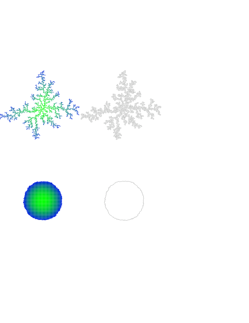
Figure 3: Clusters (left) and their boundaries (right) for the pure exterior ($\lambda=1$) problem (top) and the pure interior problem $\lambda=0$ (bottom). To visualize the time dynamics, we prescribe colors to cluster particles. The color ranges from green to blue, depending on time (or step) at which the particle joined the cluster (green for the initial step, blue for the final step)

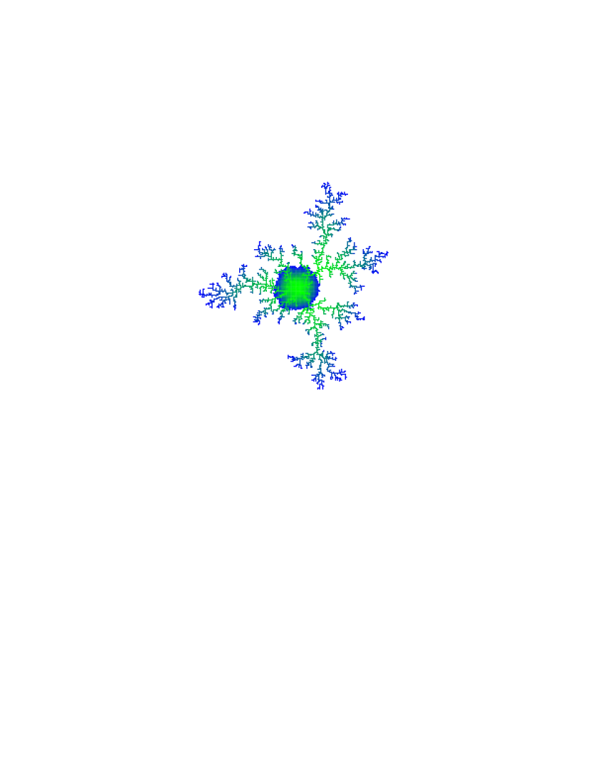
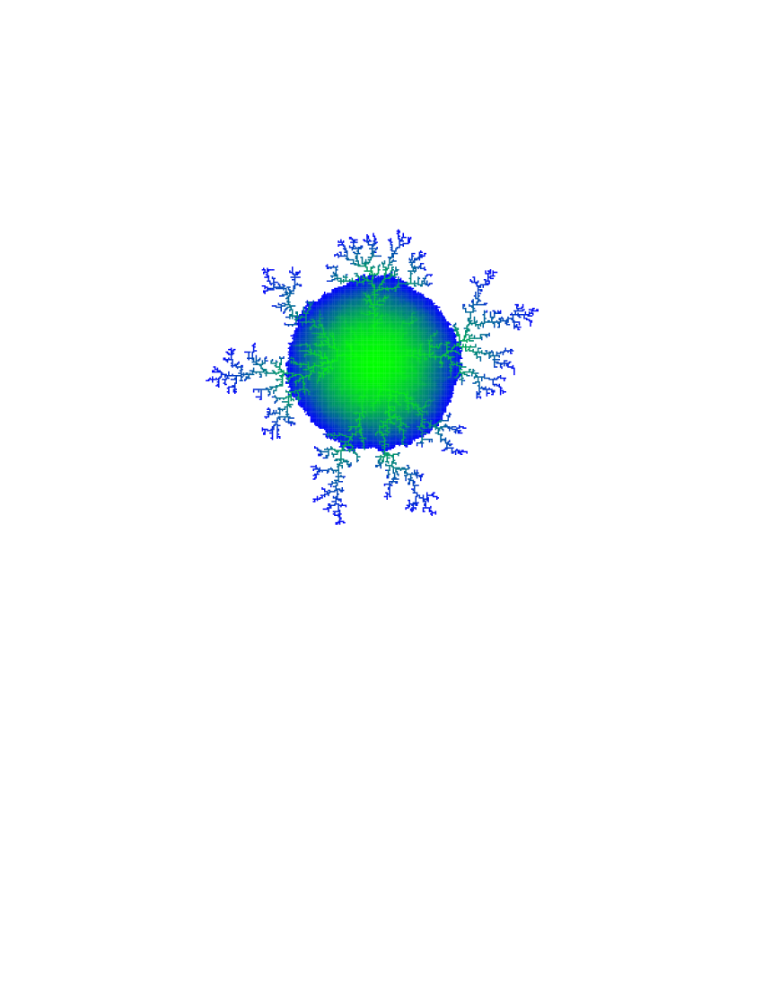
Figure 4: Examples of clusters growing from a single particle for $\lambda=0.25$ (top) and $\lambda=0.65$ (bottom)

Since in the case of pure exterior $\lambda=0$ problem the model under consideration differs from other discretizations of the Laplacian Growth by local details only, we have to expect the qualitative behavior to be similar to that of Diffusion Limited Aggregation. Indeed, for $\lambda=0$ one observes the pure fractal growth (see Figure 3). Numerical calculations give the following estimate for Hausdorff dimension of fractal boundary of a tree-like cluster (see Appendix for details of numerical calculations)

$$d=1.64\pm 0.02$$ (12)

Note that in the $\lambda=0$ case the dimension of the boundary coincides with that of the cluster.

In the case of the pure interior problem $\lambda=1$, the Discrete Laplacian Growth shows dynamics, close to that of its deterministic continuous counterpart: The cluster boundary is not a fractal, and tends to solution of the continuous problem as its size increases (see Figure 3). Such a behavior was expected due to stability of the interior continuous problem for expanding cluster.

Since the continuous problem (1-4) is stable for $\lambda>1/2$ (c.f. (5)) one would expect similar (close to deterministic) behavior of Discrete Laplacian Growth for such $\lambda$. This turns out not to be so: Instead, one observes separation of the growth in two fractal components, one of which is quasi-regular and the other is macroscopic, i.e. visible in continuous limit, constituting a finite fraction of the cluster. In the range $0<\lambda<1$, a big (grown from a single particle) cluster consists of a quasi-circular center and branches going out of it (see Figure 4). The Hausdorff dimension of such cluster boundary equals the same $d$ as in (12).

One can interpret such a behavior in the following way: The discrete growth can be viewed as a competition between the averaged process tending to a continuous limit, and probabilistic fluctuations. Such fluctuations drive the system beyond the linear stability region when $\lambda<1$.

5 Qualitative Analysis

One might try to explain the above fractal properties of growth in the stability region $1/2<\lambda<1$ by the fact that the cluster evolution considered so far starts rather with a single particle than with quasi-continuous macroscopic initial conditions. And indeed, to describe properly the continuous limit we have to start with a cluster of dimension 2, containing $N\to\infty$ particles. It is also necessary that, after rescaling the lattice spacing (or cluster linear size) by the factor $N^{-1/2}$, the initial boundary $\partial\Omega(t=0)$ tends to an analytic curve as $N\to\infty$. The time, which is the step number in the discrete model, is rescaled by the factor $1/N$.

Such growth process remains, nevertheless, a superposition of smooth (analytic) and macroscopic fractal components in the limit $N\to\infty$: The quasi-analytic part of the boundary $\partial\Omega(t)$ evolves as in the pure interior problem, while the quasi-analytic growth is superposed with the fractal growth of the pure exterior problem. In other words, the ”mixed” interior-exterior problem separates into interior and exterior parts in zero-lattice spacing limit.

It is easy to find the rate of growth of quasi-analytic to fractal components provided the separation always takes place for $0<\lambda<1$: The tree-like fractal part mainly grows on the tips of the ”branches”, since the exterior field $\phi_{-}$ is screened out in fjords between the branches, while the interior field $\phi_{+}$ is screened out inside the branches. Therefore, in zero-lattice spacing limit, the interior (quasi-analytic) part of the boundary evolves like there were only one logarithmic singularity

$$\phi_{+}\to\frac{-\lambda}{2\pi}\log|z|,\quad z\to 0,\quad{\rm and}\quad\phi_{-}=0,$$

while the fractal part of the curve grows as if

$$\phi_{-}\to\frac{1-\lambda}{2\pi}\log|z|,\quad z\to\infty,\quad{\rm and}\quad\phi_{+}=0.$$

The ratio of growth between the fractal and quasi-analytic parts (in number of particles per unit of time) is

$$(1-\lambda)/\lambda.$$

It is also straightforward to show that the separation always takes place for $0<\lambda<1$. Let’s consider the case when $\lambda$ is close to 1, since the separation of the fractal component here implies the separation for a smaller positive $\lambda$. Suppose again that initial cluster has a big size $N\to\infty$ and its rescaled boundary is close to an analytic curve, so the number of the boundary cites is of order $\sqrt{N}$.

Consider now a perturbation (fluctuation) of the boundary. Suppose that the fluctuation linear size (in lattice spacings) is $l$. For $\lambda$ close to $1$, the charge of the particles on the fluctuation tip (i.e. most distant from the quasi-analytic part of the boundary cites of the fluctuation) is of order $(1-\lambda)l^{1-D/2}/\sqrt{N}$, where $1\leq D\leq 2$. For instance, $D=1$ for one-dimensional, ”crack”-like fluctuations of length $l$, while $D=2$ for a ”bump”-like 2-dimensional fluctuations of diameter $l$. Charge of particles on the quasi-analytic part of the boundary is of order $1/\sqrt{N}$. A fluctuation tend to grow (rather than collapse) when the probability for a particle to join the cluster at the tip of fluctuation exceeds the probability for the quasi-analytic part of the boundary. Since the probability is proportional to the charge, from the above discussion it follows that fluctuations tend to grow when their linear size $l$ exceeds some critical value which is proportional to $(1-\lambda)^{-\frac{2}{2-D}}$. This value is asymptotically independent of cluster size $N$.

Since the critical size of fluctuation is $N$-independent, the possible number of critical fluctuations along the boundary is proportional to the boundary length $\sqrt{N}$. It then follows that starting from the close to analytic boundary, a big cluster develops critical fluctuations in the number of steps $f(\lambda)\sqrt{N}$, where $f(\lambda)$ is some function of $\lambda$ only. This number of steps corresponds to the time $t=f(\lambda)/\sqrt{N}$ in the scaling limit.

Therefore, in the $N\to\infty$ scaling limit, the cluster develops critical fluctuations in zero time and the separation of growth into the fractal and continuous components takes place immediately if $0<\lambda<1$.

6 Conclusions

In the present work we have introduced the Discrete Laplacian Growth (DLG) model and studied correlation between the stability of its continuous version and the fractal growth of boundary. The stability, turns out, does not guarantee an absence of the fractal growth. The growth process separates into superposition of ”continuous” and fractal component. In other words, in the $N\to\infty$ scaling limit, the discrete growth does not tend to solution of continuous model even if the later is stable and well-posed.

There remain a few questions to address:

1) Since, in $N\to\infty$ limit, DLG separates in two independent processes, one may think about implications of such a separation in the continuous model. For instance, whether this separation can be traced (in some, possibly ”hidden”, form) in continuous model or it is just a consequence of the discretization?

2) It is also known that both, exterior and interior problems possess an infinite number of conserved quantities (harmonic moments) in the scaling $N\to\infty$ limit [5, 6]. Does this imply (in view of the separation) existence of an infinite number of conserved quantities in ”mixed” models?

3) In this article we presented numerical estimate (12) for the fractal dimension of DLG. Although DLG differs from the Diffusion Limited Aggregation (DLA) only locally, their fractal dimensions do not coincide. This result is not unexpected, since dimension of DLA is sensitive even to the lattice type (see e.g. [3]) and can not be considered as a general characteristics of a class of models. It would be interesting to understand which quantities are universal, i.e. independent of local details of a discrete scheme.

7 Appendix

Numerical simulations of the Discrete Laplacian Growth have been performed by updating the discrete boundary (presented by a set of pairs of integer coordinates $\left(i(1),j(1)\right)$,$\left(i(2),j(2)\right)$, $\dots,\left(i(K),j(K)\right)$, where $K$ is the current boundary length) with the probability given by solutions of linear system (10,11). In this method an explicit solution of Laplace equation at each step is not needed, since the coefficients of Eq. (11) are defined by the coordinates of the boundary cites only.

The Green function (or lattice Coulomb potential) $G_{n,m}$ can be computed in several ways. To speed up the calculations, we have used the following approximation for the lattice Green function

$$G_{m,n}=\frac{1}{4\pi}\log(m^{2}+n^{2})-\frac{m^{4}+n^{4}-6m^{2}n^{2}}{24\pi(m^{2}+n^{2})^{3}}$$

when the point $(n,m)$ is in the exterior of the square $-L\leq n\leq L,-L\leq m\leq L$, and numerical solution for $G_{n,m}$ in the interior of this square (with the function value at the square boundary given by the above approximation). In this approach, the Green function is represented numerically as (computed once) $2L+1\times 2L+1$ table extended by the above equation. This approximation is very precise: for example, for $L=100$ the maximum deviation from the exact lattice Green function is of order $10^{-10}$.

We split solution of the system (10,11) in two parts:

$$\sum_{k^{\prime}=1}^{K}G_{i(k)-i(k^{\prime}),j(k)-j(k^{\prime})}q^{\rm ex}_{k^{\prime}}=1,\quad\sum_{k^{\prime}=1}^{K}G_{i(k)-i(k^{\prime}),j(k)-j(k^{\prime})}q^{\rm in}_{k^{\prime}}=G_{i(k),j(k)}$$

$$q_{k}=-Cq^{\rm ex}_{k}+\lambda q_{k}^{\rm in},\quad C=-\frac{1-\lambda\sum_{k=1}^{K}q_{k}^{\rm in}}{\sum_{k=1}^{K}q_{k}^{\rm ex}},$$

where $q_{k}$ stands for $q_{i(k),j(k)}$. The $K\times K$ matrix $G_{i(k)-i(k^{\prime}),j(k)-j(k^{\prime})}$ is symmetric and positive definite, so we made use of the rapidly converging conjugate gradient method [4] for the numerical solution.

Acknowledgement

The authors would like to acknowledge useful information and help received from Professor V.Kravtsov.

References

- [1] D. Bensimon, L. Kadanoff, S. Liang, B. Shraiman, C. Tang, Viscous flows in two dimensions, Rev. Mod. Phys. 58 (1986) 977.
- [2] J.Gollub, J. Langer, Pattern formation in non equilibrium physics, Rev. Mod. Phys. 71 (1999) 396-404
- [3] T. Halsey, Diffusion limited aggregation: a model for pattern formation, Physcis Today 53 (2000) 36
- [4] Kendell A. Atkinson (1988), An introduction to numerical analysis (2nd ed.), Section 8.9, John Wiley and Sons. ISBN 0-471-50023-2
- [5] S. Richardson, Hele Shaw flows with a free boundary produced by the injection of fluid into a narrow channel. J.Fluid Mech., 56, part 4, (1972), pp.609-618
- [6] A.N. Varchenko and P.I. Etingof, Why the boundary of a round drop becomes a curve of order four, American Mathematical Society, University Lecture Series, 3, (1994)
- [7] T. Witten and L. Sander, Diffusion limited aggregation: a kinetic critical phenomenon, Phys. Rev. Lett. 47 (1981) 1400