Lifetime statistics in transitional pipe flow

Abstract

Several experimental and numerical studies have shown that turbulent motions in circular pipe flow near transitional Reynolds numbers may not persist forever, but may decay. We study the properties of these decaying states within direct numerical simulations for Reynolds numbers up to 2200 and in pipes with lengths equal to 5, 9 and 15 times the diameter. We show that the choice of the ensemble of initial conditions affects the short time parts of lifetime distributions, but does not change the characteristic decay rate for long times. Comparing lifetimes for pipes of different length we notice a linear increase in the characteristic lifetime with length, which reproduces the experimental results when extrapolated to 30 diameters, the length of an equilibrium turbulent puff at these Reynolds numbers.

I Introduction

In several shear flows such as plane Poiseuille, plane Couette Bottin and Chaté (1998); Barkley and Tuckerman (2005) and also pipe flow Grossmann (2000); Mullin and (eds); Kerswell (2005); Eckhardt et al. (2007); Eckhardt (2008) turbulent dynamics is observed for flow speeds where the laminar profile is still stable against infinitesimal perturbations. In such a situation a finite amplitude perturbation is required to drive the system from laminar to turbulent flow Grossmann (2000); Boberg and Brosa (1988), and one might expect that also for the converse process, returning from the turbulent dynamics to the laminar one, a sufficiently large perturbation on top of the turbulent dynamics should be required. Several observations in direct numerical simulations and experiments show, however, that turbulent motion returns to the laminar flow suddenly and without any noticeable precursor or perturbation Brosa (1989); Darbyshire and Mullin (1995); Faisst and Eckhardt (2004); Hof (2004). From the point of view of nonlinear dynamics such a behavior suggests that the turbulent state does not correspond to a closed off turbulent attractor but rather to an open turbulent chaotic saddle Brosa (1989); Schmiegel and Eckhardt (1997); Faisst and Eckhardt (2004). One can then assign to each initial flow state a lifetime, i.e. the time it takes for this state to return to the laminar profile. The lifetime is a valuable observable that has previously been used to extract information about states on the border between laminar flow and turbulence Skufca et al. (2006); Schneider et al. (2007a). We will here use it to extract information about the turbulent dynamics itself, thereby extending the work reported in Ref. Faisst and Eckhardt (2004).

Experiment and simulations show that neighboring trajectories can have vastly different lifetimes, so that the lifetime is rather unpredictable and depends sensitively on the initial perturbation, see e.g. Darbyshire and Mullin (1995); Faisst and Eckhardt (2004); Moehlis et al. (2004). This strong sensitivity on initial conditions is consistent with observations on other transiently chaotic systems and suggests that rather than looking for the unpredictable behavior of individual trajectories, it is better to look for more reliable and stable properties derived by averaging over ensembles of initial conditions. Prominent among such properties is the distribution of lifetimes, obtained from many runs with similar but not identical initial conditions. The theoretical prediction for a hyperbolic saddle is that the probability of decay is constant in time and independent of when the flow was started, giving for the distribution of lifetimes an exponential, as in radioactive decay Kadanoff and Tang (1984); Kantz and Grassberger (1985); Tél (1991). Other functional forms are possible as well (see e.g., Tél and Lai (2008); Eckhardt and Faisst (2004)), but for the most part observations in transitional shear flows are compatible with an exponential Faisst and Eckhardt (2004); Hof et al. (2006); Mullin and Peixinho (2006a); Peixinho and Mullin (2007); Bottin and Chaté (1998); Lagha and Manneville (2007).

An exponential distribution is characterized by a characteristic decay rate or a characteristic lifetime $\tau$ which is the time interval over which the survival probability drops by $1/\mbox{e}$. How this lifetime varies with Reynolds number is currently under debate Hof et al. (2006); Peixinho and Mullin (2006); Willis and Kerswell (2007). If $\tau$ diverges at a finite Reynolds number, there is a critical value $\mathrm{Re}_{c}$ above which turbulent flow does not relaminarize but persists forever. Such a divergence would imply that the system undergoes a transition from a transient chaotic saddle to a permanently living chaotic attractor in some form of ‘inverse boundary crisis’ Grebogi et al. (1982). However, if $\tau$ does not diverge, turbulence in a pipe remains transient for all $\mathrm{Re}$. The chaotic saddle does not close to form an attractor and the turbulent ‘state’ stays dynamically connected to the laminar profile even at Reynolds numbers higher than the ones where ‘natural transitions’ are reported to occur. This might open up new avenues for controlling turbulent motion.

The prediction of an exponential distribution of lifetimes is an asymptotic one, valid for long times. On short times the distributions may follow a different functional form, as evidenced by the non-exponential parts in almost all distributions published so far. Moreover, the results may depend on additional parameters, such as an aspect ratio or the length of the pipe. The dependence on these parameters has not been studied so far. It is our purpose here to discuss some of these effects for transitional pipe flow.

We begin in section II with a survey of previous experimental and numerical results. Section III then is devoted to an analysis of three effects: the dependence on the ensemble of initial conditions in section III.2, the variation of the characteristic lifetime with $\mathrm{Re}$ in III.3 and the variation with the length of the pipe in section III.4. We conclude with a summary and outlook in section IV.

II Survey of results

As usual, the mean downstream velocity $\langle{u}\rangle$, the diameter $D$ of the pipe and the viscosity $\nu$ of the fluid can be combined into the dimensionless Reynolds number,

$$\mathrm{Re}=\frac{\langle{u}\rangle D}{\nu}\,.$$ (1)

The pipe diameter $D$ and the velocity $\langle{u}\rangle$ then define a unit of time $D/\langle{u}\rangle$. Since the flow moves downstream with the mean velocity $\langle u\rangle$, time can be translated into distance traveled, so that the distance in units of the diameter equals the time $t$ in units of $D/\langle{u}\rangle$. Because of this relation between length and time, it is crucial to work with very long pipes so that the observation times become as large as possible.

When the flow becomes turbulent, the friction factor increases. Therefore, either the forcing (pressure drop) has to increase so as to maintain the mean flow speed, or the mean flow speed will decrease, perhaps reducing the Reynolds number so much that the flow relaminarizes Mellibovsky and Meseguer (2007). Thus, many modern experiments work with a constant flow rate Darbyshire and Mullin (1995), or with very long pipes Hof et al. (2006), in which the change in Reynolds number becomes negligible as long as the turbulence remains confined to a small section of the pipe: In the range of Reynolds numbers studied here, the turbulence is localized in a region of about 30D length Wygnanski and Champagne (1973). To measure lifetime statistics one can either follow a puff on its journey down the pipe and determine the downstream position where it decays; or one can choose a fixed downstream position, which corresponds to a fixed lifetime, and measures the probability that puffs survive the journey down the pipe up to this chosen point.

The first approach was chosen by Mullin in a recent series of experiments Mullin and Peixinho (2006b, a); Peixinho and Mullin (2006, 2007) inspired by the numerical studies in Faisst and Eckhardt (2004). In a first group of experiments Mullin and Peixinho (2006b) the decay of the perturbation could be detected with a camera that traveled with the perturbation downstream. The length of the pipe allowed for a maximal observation time of 500 units. The flow was perturbed by injecting six jets of different amplitudes, and $40$ to $100$ independent repetitions were taken for each Reynolds number. The asymptotic regime of the distributions of lifetimes was found to follow a law

$$P(t)\sim\exp\left(\frac{t-t_{0}}{\tau(\mathrm{Re})}\right)\;,$$ (2)

with a characteristic lifetime $\tau(\mathrm{Re})$ depending on $\mathrm{Re}$ and an initial offset $t_{0}\approx 100\ldots 150$ before which no decay was observed. The strong increase of the characteristic lifetime with $\mathrm{Re}$ lead to the conclusion that it diverges at a finite critical Reynolds number. For the critical Reynolds number they give in Mullin and Peixinho (2006b) the values $\mathrm{Re}_{c}=1710\pm 10$ and $\mathrm{Re}_{c}=1830\pm 10$, and in Mullin and Peixinho (2006a) the values $\mathrm{Re}_{c}=1695\pm 20$ and $\mathrm{Re}_{c}=1820\pm 20$, for two different kinds of perturbations, described as ‘strong’ and ‘weak’ types of perturbation, respectively. In an effort to address the dependence on the type of initial perturbations, they performed a second experiment with a slightly different perturbation protocol Peixinho and Mullin (2006): In order to obtain more generic initial conditions the system was started at a higher flow speed, a perturbation that triggered turbulence was introduced and then the Reynolds number was reduced to the one for which lifetime statistics were collected. This gives another sample of initial conditions but limits the remaining observation time to less than 450. With such a perturbation the characteristic lifetimes were compatible with

$$\tau(\mathrm{Re})\propto(\mathrm{Re}_{c}-\mathrm{Re})^{-1\pm 0.02}\,,$$ (3)

but now with a different critical Reynolds number of $\mathrm{Re}_{c}=1750\pm 10$.

It is difficult to model the perturbations induced by jets in numerical simulations (Mellibovsky and Meseguer (2007)), but it is relatively straightforward though time-consuming to imitate the second protocol of Mullin, where the initial conditions are taken from a turbulent flow at higher Reynolds numbers. Willis and Kerswell Willis and Kerswell (2007) did just that for five different Reynolds numbers and concluded that $Re_{c}=1870$, as suggested by some experiments. However, when the analysis of their data points is corrected as suggested in Hof et al. (2007), the demonstration of a divergence is less convincing and the data become compatible with the results of Hof et al Hof et al. (2006).

The experiments by Hof et al. Hof et al. (2006) just mentioned use a different approach. In a pressure driven flow through a thin pipe of only $4$ mm diameter but $30$ m length they realized dimensionless observation times of up to 7500 units. Since the flow could not be visualized, the time and position of decay could not be determined directly. However, a laminar and a turbulent patch in the flow can easily be distinguished once they leave the pipe, so that it is relatively easy and straightforward to determine whether the flow has stayed turbulent until it exits the pipe. Therefore, they could determine the probability to be turbulent after a time period given by the distance between the perturbation and the outlet, as a function of flow rate. This gives $P(t,\mathrm{Re})$ as a function of $\mathrm{Re}$ for $t$ fixed. Collecting data for different $t$ then gives the parameters in the lifetime distribution including the Reynolds number dependence. For short times, the data are within the error bars of Peixinho and Mullin (2006), but for longer times they deviate from the divergent behavior implied by (3). Instead, it was found that the lifetimes are well represented by an exponential variation,

$$\tau^{-1}(\mathrm{Re})\propto\exp(a+b\mathrm{Re})$$ (4)

with $a=55.3$ and $b=-0.032$.

III Lifetime distributions and their properties

In this section we study lifetime distributions in pipe flow within direct numerical simulations. Since the calculations are extremely time consuming, we will not aim to repeat the puff simulations of Willis and Kerswell (2007), but rather focus on short, periodically continued pipe sections, and then discuss how these results scale up to turbulence in regions of the length of turbulent puffs. In the next subsection we first discuss features of individual turbulent trajectories, before turning to the ensemble dependence of lifetime distributions, the variations with Reynolds number and the length dependence.

Individual trajectories were generated using the pseudospectral DNS code developed in Schneider (2005) and already used in our previous studies Hof et al. (2006); Schneider et al. (2007a, b); Eckhardt et al. (2007). Simulations of elongated puffs with the determination of their travel velocity, envelope and internal dynamics are given in Schneider and Eckhardt (2008). The code uses Fourier modes in downstream and azimuthal direction and Chebyshev polynomials in the radial direction, and a projection method to eliminate the pressure. The simulations on pipe segments presented in this section are carried out with $n$ Fourier modes in azimuthal and $m$ Fourier modes in downstream direction, where ${|n|}/{N_{max}}+{|m|}/{Z_{max}}\leq 1\,$ with $N_{max}=16$ and $Z_{max}$ increasing from $14$ for the ‘short’ pipe of length $5D$ to $Z_{max}=25$ and $Z_{max}=45$ for the ‘medium’ ($L=9D$) and ‘long’ ($L=15D$) pipes, respectively. Consequently, we consider up to $33$ Fourier modes in azimuthal direction. In downstream direction up to $31$ modes are considered for the short, $51$ for the medium and $91$ for the longest pipe. We use $49$ Chebyshev polynomials for the expansion in the radial direction. This moderate resolution results from a compromise of accurate representation of the dynamics and maximum simulation speed, required for good statistics.

III.1 Features of individual trajectories

Consider a perturbation of the laminar Hagen-Poiseuille flow applied at time $t=0$. The evolution of the initial condition $\vec{u}(t=0)$ can be followed in time until it decays or reaches the maximum integration time in a simulation or leaves the pipe in an experimental setup. Fig. 1 shows the evolutions of four different but similar initial conditions. As an indicator for the turbulent intensity, we take the energy of the three-dimensional structures,

$$E_{3D}=\left({\sum_{m\neq 0}\int_{\text{Vol}}\vec{v}^{2}_{n,m}\mathrm{d}V}\right)\left/\left({\int_{\text{Vol}}4(1-r^{2})^{2}\mathrm{d}V}\right)\right.\;,$$ (5)

where $\vec{v}^{2}_{n,m}$ denotes the $(n,m)$-Fourier mode if the perturbation field $\vec{v}=\vec{u}-2(1-r^{2})\vec{e}_{z}$ is decomposed into Fourier modes in azimuthal ($m$) and axial ($n$) direction. The energy content of the streamwise modulated Fourier modes is normalized by the kinetic energy of the laminar profile.

Since a flow field only asymptotically reaches the laminar profile exactly, ‘decay’ is defined as reaching a situation where perturbations of the laminar profile are so small that the further evolution follows an exponential drop off. Any perturbation is therefore characterized by a lifetime that slightly depends on the chosen criterion to detect being close to the laminar profile. Technically, one introduces a cut-off threshold either on the kinetic energy stored in the deviation from the laminar profile $\int||\vec{u}-2(1-r^{2})\vec{e}_{z}||^{2}\mathrm{d}V$, or on the kinetic energy (5) stored in streamwise invariant Fourier modes only. The threshold on these energies is chosen such that the further evolution can be described by the linearized equations, so that the system cannot return to the turbulent dynamics. The lifetime then is defined as the time it takes to reach this target region around the laminar profile.

Figure 1: (Color online) Simulated evolution of four initial disturbances at $\mathrm{Re}=1900$ in a periodic pipe of length $L=15D$. Plotted is the kinetic energy of the deviation from the laminar profile that is stored in the streamwise varying Fourier modes, eq. 5. Initial conditions are constructed from a modulated Zikanov mode discussed in the main text. The four initial conditions differ by less than $0.5\%$ in energy content. The pertubations first grow in energy and show an overshoot before settling down to the turbulent state. They then suddenly decay without any prior indication and the energy of the perturbation decays monotonically. The chosen criterion for decay is based on the energy threshold $E_{3D}<5\times 10^{-5}$.

III.2 Ensemble dependence

Now consider an ensemble of several different but similar perturbations. The collection of individual lifetimes can be used to estimate the probability $P(t)$ to still be turbulent at some time $t$. A chaotic saddle should give rise to exponential asymptotic tails of this distribution that are independent of the choice of initial conditions but characteristic for the saddle.

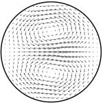
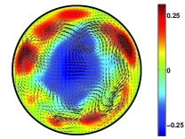
Figure 2: (Color online) Spatial structure of the types of initial perturbations considered. Left panel: In plane velocity components of Zikanov’s nearly optimal growing mode. Axial velocity components vanish. The translational symmetry of Zikanov’s mode is broken by applying a $z$-dependent twist. Right panel: Cross-section of a velocity field from a turbulent run at $\mathrm{Re}=2150$. The vector plot indicates the in-plane motion. Color coding is used for the axial velocity relative to the laminar parabolic profile.

One type of perturbations we consider here is a pair of vortices as in the optimally growing modes identified by Zikanov Bergström (1993); Schmid and Henningson (1994); Zikanov (1996). In order to break translational symmetry they are modulated in streamwise direction by applying a $z$-dependent twist:

$$\vec{u}_{0}(r,\varphi,z)=\vec{u}_{\text{Zik}}\left(r\,,\varphi+\varphi_{0}\sin\left(\frac{2\pi}{L}z\right),\,z\right)\;,$$ (6)

where $\vec{u}_{\text{Zik}}$ is Zikanov’s mode and $L$ is the length of the computational domain used in our direct numerical simulation. The spatial structure is presented in Fig. 2. Mimicking experimental protocols, where the spatial structure of the perturbation is prescribed by the setup, the ensemble of initial conditions is constructed by varying the amplitude of the twisted Zikanov mode. A second type of perturbation is a snapshot from a turbulent run at $\mathrm{Re}=2150$ which is scaled in energy i.e., in amplitude. A cross-section is shown in Fig. 2.

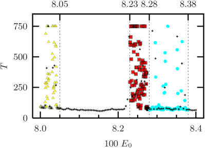
Figure 3: (Color online) Lifetime of initial conditions at $\mathrm{Re}=1900$. The pipe is $L=15D$ long. The initial conditions are constructed from a turbulent snapshot of a $\mathrm{Re}=2150$ run (Fig. 2). It is scaled in kinetic energy $E_{0}$. The black crosses belong to an ensemble constructed by varying the energy form $E_{0}=8\times 10^{-2}$ to $E_{0}=8.4\times 10^{-2}$ in $100$ equidistant steps. Additional ensembles with $100$ samples each focus on regions of high probability to observe long turbulent transients. The yellow triangles indicate an ensemble that ranges form $E_{0}=8.0\times 10^{-2}$ to $E_{0}=8.05\times 10^{-2}$ in $100$ steps. The red squares are located in the range between $E_{0}=8.23\times 10^{-2}$ and $E_{0}=8.28\times 10^{-2}$. Finally the cyan circles reach from $E_{0}=8.28\times 10^{-2}$ to $E_{0}=8.38\times 10^{-2}$. The corresponding lifetime distributions for all ensembles are shown in Fig. 4.

Fig. 3 shows the lifetime of the perturbation as a function of the initial energy $E_{0}$. Regions of small and smoothly varying lifetime are clearly separated from regions of longer fluctuating lifetimes. In regions with short lifetimes the flow relaxes quickly to the laminar profile. Towards the boundaries of these regions the lifetimes increase quickly and reach plateaus at the maximal integration time. Magnifications of the plateau regions show chaotic and unpredictable variations of lifetimes Faisst and Eckhardt (2004). The cliff-structure in the lifetime is due to the geometric features of the basin of attraction of the laminar profile and has been seen in pipe flow Schneider et al. (2007b) and low-dimensional representations of shear flows Moehlis et al. (2004, 2005); Skufca et al. (2006).

A first ensemble of initial conditions is constructed by varying the energy from $E_{0}=8.0\times 10^{-2}$ to $E_{0}=8.4\times 10^{-2}$ in $100$ equidistant steps. Other ensembles are chosen such that they provide a higher resolution in initial energies for the regions where high lifetimes are expected.

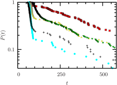
Figure 4: (Color online) Lifetime distribution for fixed parameters ($\mathrm{Re}=1900$ and periodic domain of length $L=15D$) for different ensembles of initial conditions. Presented is data obtained from an ensemble of $200$ samples constructed from twisted Zikanov modes (green down-facing triangles). The other ensemble result from scaling a turbulent flow field from a $\mathrm{Re}=2150$ run. The black crosses indicate an ensemble constructed from scaling the energy of the field from $E_{0}=8\times 10^{-2}$ to $E_{0}=8.4\times 10^{-2}$ in $100$ equidistant steps. The lifetime as a function of this energy shows typical folds (see Fig. 3). Based on this fold structure remaining ensembles indicated by the yellow triangles, red squares and cyan circles are tailored towards reaching the saddle i.e., additional runs were chosen in the ‘right’ energy region. The specific ensembles containing $100$ samples each are described in Fig. 3 where the same symbols are used. While the initial part of the distributions depends both in length and functional form on the chosen ensemble, the slope of exponential tails is universal within the limits of statistical accuracy.

Fig. 4 shows $P(t)$ for fixed $\mathrm{Re}$ calculated for the different ensembles of initial conditions. Each individual distribution is characterized by an initial offset $t_{0}\approx 75$ where no trajectory decays. Then one observes a middle part that both in length and functional form differs among the various ensembles before asymptotically exponential tails are reached. Within the limits of statistical uncertainties the decay rates (i.e., the slopes in a semi-logarithmic plot) are independent of the ensemble of initial conditions and encode a characteristic feature of the chaotic saddle.

In view of the cliff-structure in lifetime the origin of the non-universal middle part becomes obvious: Only trajectories starting from the regions of fluctuating lifetime reach the chaotic saddle from which they can decay at a characteristic rate. Initial conditions from the regions in between directly decay without having reached the saddle which leads to the non-universal initial parts of $P(t)$ in Fig. 4. The different plots in Fig. 4 correspond to different ensembles chosen from all possible initial conditions presented in Fig. 3.

We now focus on the initial offset time $t_{0}$. It corresponds to the smallest time it takes for an initial condition from the chosen ensemble to decay. It evidently depends on the initial perturbation. In particular, this time scale can in principle be arbitrarily close to zero by including an arbitrarily small perturbation to the linearly stable laminar profile in the ensemble. However, ‘typical’ perturbations used both in simulations and lab experiments are characterized by a typical initial formation time $t_{0}$ (with $t_{0}\approx 100\ldots 150$ in experiments). This can be rationalized as follows:

We first note that $t_{0}$ is large compared to the Lyapunov time measured in the turbulent motion Faisst and Eckhardt (2004), which gives a typical timescale for the dynamical separation of neighboring trajectories on the saddle. However, a trajectory does not necessarily start on the chaotic saddle. Its initial condition is a flow field that hopefully initiates turbulence i.e., the trajectory approaches the chaotic saddle, but typically it does not belong to the saddle itself. In addition a trajectory starting its decay from the saddle has to follow the evolution through state space until it ends up in the vicinity of the laminar profile. Consequently the offset $t_{0}$ contains two parts: The formation time $t_{\text{for}}$ required to reach the turbulent ‘state’ and the decay time $t_{\text{dec}}$ it takes to finally reach the neighborhood of the laminar state after the decay has been initiated. This can also be directly observed in Fig. 1. The presented energy traces consist of three parts: the initial energy growth, the chaotic fluctuations indicating turbulent dynamics on the saddle, and the decay towards the laminar state.

As discussed in Section II the decay time can be estimated from experimental observations that a puff decays while traveling about $50D$ downstream Hof (2004). This translates into a time $t_{\text{dec}}\approx 50$. Theoretically it follows from the mechanism of decay: It starts first with a reduction of transverse modulations leading to a break out of the regeneration cycle supporting turbulent motion Waleffe (1997) and then shows a viscous damping of streamwise deviations from from the laminar profile.

The formation time $t_{\text{for}}$ can be estimated from the experimental observation that is takes $t_{\text{for}}$ about $40$ for a perturbation (jet injection Hof (2004)) to develop into an equilibrium puff. It is also observed in simulated short periodic pipes: Taking an initial condition that contains pairs of counter-rotating vortices in axial direction such as Zikanov’s almost optimally growing mode, these small perturbations grow in energy by generating strong streaks in a so called lift-up process driven by the non-normality of the Navier-Stokes operator Waleffe (1995). The generated streaks then become unstable, transverse vortices appear and the flow turns turbulent. The formation time can therefore be estimated by the growing period of a Zikanov mode and originates from the non-normal character of the Navier-Stokes operator.

The discussed mechanism is also present in experiments where the flow is perturbed by injecting fluid jets perpendicular to the pipe Panton (2001). These jets give rise to pairs of counter-rotating vortices that will draw energy from the base profile and grow by the same mechanism observed in the dynamics of a streamwise independent Zikanov modes. The experimental observation agrees with typical formation times of equilibrium puffs in simulations in a periodic pipe of length $L=50D$ where a localized form of Zikanov’s mode was used as an initial condition.

We thus conclude that the specific choice of initial conditions affects the functional form of the lifetime distribution for small times. Both the initial time offset $t_{0}$ and the middle part of the lifetime distribution depend on the chosen ensemble of initial conditions. Universal properties of the turbulent state are only encoded in the asymptotic tails, which result from trajectories that actually reach the turbulent state before their decay. The exponential form of these tails is compatible with a chaotic saddle in state space and characteristic decay rates can be ‘measured’ by fitting exponentials to the asymptotic tails of the lifetime distributions.

In order to probe the chaotic saddle, i.e., analyze the universal asymptotic part of the distribution and minimize the high computational costs at the same time, it is favorable to choose an ensemble of initial conditions that is likely to reach turbulence. Modulated Zikanov modes seem to be a good choice whereas independent snapshots from a turbulent run at slightly higher $\mathrm{Re}$ tend to decay directly. This can for example be observed by comparing the lifetime distributions (Fig. 4) of the ensembles constructed by scaling the turbulent flow field and the Zikanov mode respectively. Although snapshots from runs at higher Reynolds number are complex and appear to be ‘turbulent’ they need not be located close to the chaotic saddle in the state space of the system at slightly lower $\mathrm{Re}$. Typical length and time scales of turbulent motion change with $\mathrm{Re}$ so that turbulent snapshots at one Reynolds number might not ‘fit’ the dynamics at another $\mathrm{Re}$ . In contrast, in the case of Zikanov modes the flow has enough time to adapt to the dynamics of the Navier-Stokes equations. Moreover, the Zikanov mode shares a characteristic pair of streamwise vortices with the edge state of pipe flow Schneider and Eckhardt (2006); Schneider et al. (2007b). Since the edge state is located in-between the laminar state and the chaotic saddle, an initial condition close to the edge state should be especially efficient in initiating turbulence.

To summarize: The specific form of a lifetime distribution does not only depend on the system parameters such as Reynolds number and — in the case of a simulation — length of a periodic domain and resolution of the numerical representation that completely define the dynamical system. $P(t)$ also depends on the ensemble of initial conditions. The large initial offset due to transient growth of initial perturbations and the initial drop generated by trajectories that decay directly without reaching the chaotic ‘state’ are not universal. In view of the cliff-structure in lifetime that shifts with Reynolds-number even choosing the same ensemble of initial conditions does not prevent complicated variations of the non-universal parts of $P(t)$ with $\mathrm{Re}$. Only the exponential tails in the asymptotic regime of the lifetime distribution carry information about the chaotic saddle and its characteristic decay rate. Consequently, long observation times reaching into the asymptotic range and initial conditions that have a high probability to reach turbulent dynamics are needed in any study of characteristic lifetimes.

III.3 Reynolds number dependence $\tau(\mathrm{Re})$

Lifetime experiments were performed in periodic domains of length $L=5D$, $L=9D$ and $L=15D$ for various Reynolds numbers. The ensemble of initial conditions was constructed from twisted Zikanov modes of varying amplitude. For each Reynolds number at least $100$ independent trajectories were integrated up to a maximum integration time of $3000R/U_{cl}=750D/\langle{u}\rangle$ which is about twice the observation time available in the Manchester pipe and a tenth of the maximal observation time in the discussed experiments by Hof. Characteristic lifetimes were extracted from the slopes of exponentially varying tails of the measured lifetime distributions.

Fig. 5 shows the probability $P(t)$ to still be turbulent at some time $t$ as a function of this time for the ‘short’ $L=5D$ pipe. The data points lie on straight lines in a semi-logarithmic plot, clearly indicating an exponential variation for large times. The slopes of the indicated fits which correspond to $1/\tau$ with $\tau$ the characteristic timescale of the decay process are plotted in Fig. 6 as a function of the Reynolds number.

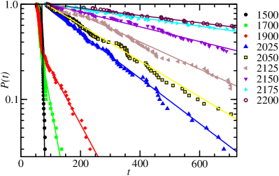
Figure 5: (Color online) Probability $P(t)$ to still be turbulent after some time $t$ for the ‘short’ $L=5D$ pipe. For each Reynolds number (given in the legend) $100$ independent initial conditions have been integrated up to a maximum integration time of $750$. Exponential fits to the tails of the distribution are indicated by straight lines in the semi-logarithmic representation. The measured slopes are shown in Fig. 6.

Figure 6: (Color online) Inverse characteristic lifetimes $\tau^{-1}$ for the ‘short’ pipe of length $L=5D$, as extracted from the exponential fits of $P(t)$ (see Fig. 5) as a function of Reynolds number both on a semi-logarithmic (main) and a linear scale (inset). The error bars result from extreme fits still compatible with the data. Thus, they reflect both intrinsic statistical uncertainties of the exponential fits and errors resulting from estimating the beginning of the asymptotic regime. The data is compatible with an exponential variation of $\tau(\mathrm{Re})$ but does not support the linear scaling proposed in the literature before (cf. inset). Thus, the data does not support a divergence of $\tau$ i.e., a zero crossing of $1/\tau$ at a finite Reynolds number close to $2000$.

The characteristic lifetime $\tau$ increases rapidly with $\mathrm{Re}$ which, in previous studies Faisst and Eckhardt (2004); Mullin and Peixinho (2006b); Peixinho and Mullin (2006), led to the conclusion that it diverges at a finite critical Reynolds number $\mathrm{Re}_{c}$ like

$$\tau(\mathrm{Re})\sim\frac{1}{\mathrm{Re}_{c}-\mathrm{Re}}\;.$$ (7)

In a linear plot of the inverse lifetime $1/\tau$ as a function of $\mathrm{Re}$ this would correspond to a linear variation that crosses zero at the critical Reynolds number. Our data do not support this scaling. Indeed, $1/\tau$ approaches zero as we increase $\mathrm{Re}$ but there is no indication of a divergence. Instead the data is compatible with an exponential scaling (4), which corresponds to a straight line in a semi-logarithmic representation. The values for the parameters $a$ and $b$ are listed in table 1.

Consequently, there is no evidence for a transition from a chaotic saddle to a permanent chaotic attractor, at least not close to a Reynolds number of order $2000$, where critical values have been reported previously.

Comparing with experimental results Hof et al. (2006), our numerical studies confirm exponential lifetime distributions and that the characteristic lifetime does not diverge but grows exponentially with the Reynolds number. However, the parameters of the exponential scaling law do not match quantitatively. This shortcoming is addressed in the next section, where we discuss how the length of the periodic domain used in our simulation affects the statistics.

III.4 Extensitivity of $\tau(\mathrm{Re})$

Having found the exponential scaling of characteristic lifetimes both in experimental works and in numerical simulation, one can quantitatively compare both systems. The main difference between both considered systems is that in an experiment one observes a localized turbulent puff traveling through a very long pipe whereas in short simulated periodic pipes not the full spatiotemporal structure but only the internal dynamics of a puff is captured. There is no coexistence of a turbulent region and laminar flow and no dynamics of the fronts of a turbulent puff. If the periodic domain becomes long compared to all internal scales of a turbulent puff, including its overall size, features of the experiment should be quantitatively recovered. For shorter computational domains, however, finite-size effects are to be expected.

We analyze the dependence on the length $L$ of the computational domain by comparing the results from the short $L=5D$ pipe with additional simulations for a ‘medium’ $L=9D$ and a ‘long’ $L=15D$ pipe. The length $L=9D$ (rather than $L=10D$) for the medium pipe was chosen such that periodic structures that might be favored by the periodicity of the small reference calculation do not exactly ‘fit’ the new period in downstream direction.

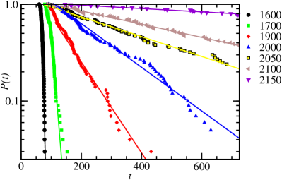
Figure 7: (Color online) Lifetime distributions for the pipe of ‘medium’ length $L=9D$ pipe. For each Reynolds number (legend) $100$ trajectories have been analyzed. The straight lines indicate exponential fits to the tails of the distributions.

Fig. 7 shows lifetime distributions based on $100$ individual runs at every Reynolds number for the medium pipe. Exponential fits to the tails are presented as straight lines in the semi-logarithmic plot.

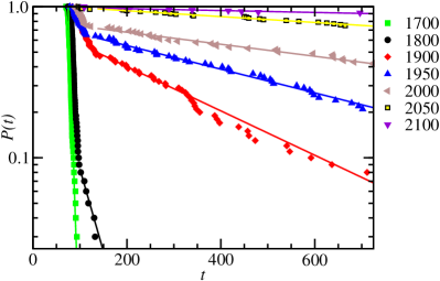
Figure 8: (Color online) Same as Fig. 7 but for the ‘long’ pipe of length $L=15D$. Note the long offset $t_{0}$ especially for $\mathrm{Re}=1900$.

Fig. 8 shows the same data also based on the analysis of $100$ runs at each Reynolds number for the long periodic pipe. In this plot, the different parts of $P(t)$ i.e., the initial decay followed by asymptotic tails that have to be used for measuring the characteristic lifetimes, are obvious.

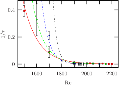
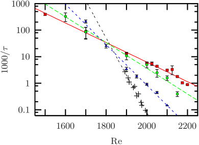
Figure 9: (Color online) Inverse characteristic lifetimes extracted from simulations in periodic domains of different length ($L=5D$ (red squares), $L=9D$ (green circles), $L=15D$ (blue triangles)) and from the experiment by Hof Hof et al. (2006) (black crosses) in a linear (left panel) and semi-logarithmic plot (right panel). The straight lines are exponential fits to the data, indicating that all data sets are individually compatible with an exponential scaling of lifetime with Reynolds number. The slope of the exponential grows with the length of the periodic domain and approaches quantitatively the experimental results. By extrapolation shown in Fig. 12 one can speculate that numerical and experimental results should match at $L=30D$, which is about the length of an equilibrium puff.

In Fig. 9 the extracted inverse characteristic lifetimes from Fig. 7 and Fig. 8 are presented together with the $L=5D$ reference data.

All three presented data sets show no evidence for a divergence. Each one is fully compatible with an exponential scaling of $\tau$ as a function of $\mathrm{Re}$. However the slope of the exponential is not universal but varies with the length of the computational domain. Large changes in the characteristic lifetime occur in a smaller interval of Reynolds numbers for a longer pipe. For Reynolds numbers larger than about $1850$ the characteristic lifetime grows with the length of the computational domain.

Hence, the characteristic lifetime is not a purely intensive measure. It scales with the size of the system under consideration. Such a scaling is compatible with the reasoning that has been developed for spatially extended transient chaos, when the domains considered are larger than the correlation length.

At the Reynolds numbers considered, the flow in the pipe is correlated in azimuthal, radial and also axial direction. The axial auto-correlation functions for the three velocity components are shown in Fig. 10. They fall off rather quickly within about $2R$. The short axial correlation length suggests that useful information about the interior dynamics of the flow can be obtained by studying relatively short domains. Specifically, for a length of $10R$ the axial correlations in the downstream fluid are down to $30$ per cent, but the computational advantages are enormous and allow for detailed studies of deterministic Faisst and Eckhardt (2003) and statistical properties Schneider et al. (2007a).

A turbulent puff, on the other hand, defined via the total energy content, and averaged over time, is much longer, see Fig. 11. Therefore, it is plausible to think of the flow in a turbulent puff as succession of segments of length $D$, which are more or less uncorrelated. Let $r$ be the probability for one of them to decay over a time interval $\delta t$. Then the probability for $N$ of them to decay simultaneously is $r^{N}$. It has to be simultaneous, for otherwise a turbulent cell could main turbulence and trigger a spreading along the axis. Since $r=1/\tau$, this implies that the lifetime $\tau_{N}$ for the system of $N$ cells is $\tau_{N}=\tau^{N}$. With the representation (4) this implies a linear increase of the parameters $a$ and $b$ with the number of cells, i.e. the length of the turbulent section. This is nicely borne out by the data in Fig. 12.

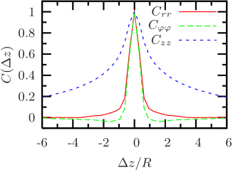
Figure 10: (Color online) Autocorrelation functions for the downstream ($C_{zz}$), azimuthal ($C_{\varphi\varphi}$) and radial ($C_{rr}$) velocities along the pipe axis. The correlations are evaluated in the comoving frame of reference of a turbulent puff Schneider and Eckhardt (2008) and are normalized to one for vanishing axial shift $\Delta z$.

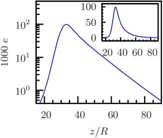
Figure 11: (Color online) Energy content of a turbulent puff, averaged over time in a co-moving frame (as discussed in Schneider and Eckhardt (2008)) in a logarithmic representation (main panel) and a linear on (inset). The rapid, exponential drop of underlines the strong localization properties of a turbulent puff and also shows that its length is rather well defined to be about 30 D. The spot moves from left to right.

Comparing with the characteristic lifetimes extracted from the experiments by Hof included in Fig. 9 the lifetimes extracted from simulations quantitatively approach experimental values as one increases the length of the computational domain.

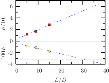
Figure 12: (Color online) The variation of inverse lifetime shown in Fig. 9 may be described as $\tau^{-1}=\exp(a+b\;\mathrm{Re})$ with two parameters $a$ and $b$. We plot these parameters as a function of the length $L$ of the computational domain. The red boxes correspond to the parameter $a/10$ and the yellow circles to $100b$. The experimental values from Hof et al. (2006) are indicated by the green dashed horizontal lines. Linear fits to the data points (blue dashed lines) reach the experimental values at approximately the same length $L\approx 30D$ which is about the length of an equilibrium puff.

The individual exponential variation of the lifetime with $\mathrm{Re}$ may be described using (4) with two parameters $a$ and $b$ which depend on the length $L$ of the computational domain. In Fig. 12 we plot these parameters as a function of $L$. Linear extrapolation shows that both parameters independently approach the experimental values – included as horizontal lines in Fig. 12 – at the same length. A quantitative match between experimental and numerical results can thus be expected at a length of $L=30D$, which is approximately the length of equilibrium puffs observed in long pipes. Hence, the data suggests that the characteristic lifetime is an extensive quantity scaling with the length of a turbulent patch.

$L/D$	$a$	$100b$
$5$	$11.9$	$-0.85$
$9$	$16.7$	$-1.11$
$15$	$28.0$	$-1.76$
30 (extrap.)	$52.1$	$-3.11$
experiment	$55.2$	$-3.23$

Table 1: Parameters for the exponential law (4). The top three rows are from numerical simulations of periodic sections of length $L=5D$, $9D$ and $15D$, respectively. The next to last line gives the value extrapolated for $L=30D$ and the last row gives the experimental data of Hof (2004).

Our findings support the assumption that turbulent puffs do not decay from their boundaries but decay is initiated in the bulk region. Short periodic pipes appear to faithfully reproduce the internal dynamics of a turbulent puff and the dynamics of the fronts is of minor importance.

IV Conclusions

The results presented here confirm that lifetime distributions of turbulent pipe flow asymptotically follow exponentials. While there may be differences for short times, the long time behavior is robust. This observation supports the idea that turbulent motion is generated by a chaotic saddle in state space. Features of the measured probability functions can be explained in terms of an ensemble of initial conditions that either directly decay or reach the strange chaotic saddle. From this saddle, trajectories decay at a constant escape rate, i.e., independent of the previous state. This situation is analogous to that of a particle moving in a complex box with some holes through which it can decay Ott (2002); Faisst and Eckhardt (2004), or an unstable nucleus subject to radioactive decay. After escaping from the saddle trajectories then follow the slow dynamics towards the linearly stable laminar profile.

A thorough analysis of lifetime distributions from both experimental and numerical studies of pipe flow as well as plane Couette flow shows that the characteristic lifetimes grow with Reynolds number, but that they do not diverge at a finite value of Reynolds numbers. As a consequence, there is no evidence that the chaotic saddle in state space turns into an attractor by some sort of ‘inverse boundary crisis’ Ott (2002). Even for Reynolds numbers exceeding $2000$ turbulent signals consist of transients that decay finally, though the time for decay can be very long. As regards much higher Reynolds numbers and in particular the transition from puffs to slugs which increase in length, the present results suggest that also the decay time $\tau(Re)$ may become longer. But this is insufficient to suggest a transition to a permanent attractor, so that the question about a global bifurcation that turns the turbulent dynamics into an attractor remains open. In any case, the fact that turbulent motion stays dynamically connected with the laminar profile at Reynolds numbers exceeding $2000$ suggests that turbulent flow could be intentionally laminarized at minimal energetic costs.

An intriguing finding of the present study is a dependence of the characteristic lifetimes on the spatial extension of a turbulent region. The larger it is the less likely it decays. For the case of puffs, it is possible to extrapolate the present numerical results to the experimental ones. The results for pipe flow are consistent with theoretical models for spatially extended systems. It will be interesting to see to which extend the extensive scaling of lifetimes seen here in pipe flow is generic and can be found in other linearly stable flows such as plane Couette flow.

References

- Bottin and Chaté (1998) S. Bottin and H. Chaté, Eur. Phys. J. B 6, 143 (1998).
- Barkley and Tuckerman (2005) D. Barkley and L. S. Tuckerman, Phys. Rev. Lett. 94, 014502 (2005).
- Grossmann (2000) S. Grossmann, Rev. Mod. Phys. 72, 603 (2000).
- Mullin and (eds) T. Mullin and R. K. (eds), Laminar-turbulent transition and finite amplitude solutions (Springer, Dordrecht, 2004).
- Kerswell (2005) R. R. Kerswell, Nonlinearity 18, R17 (2005).
- Eckhardt et al. (2007) B. Eckhardt, T. M. Schneider, B. Hof, and J. Westerweel, Annu. Rev. Fluid Mech. 39, 447 (2007).
- Eckhardt (2008) B. Eckhardt, Nonlinearity 21, T1 (2008).
- Boberg and Brosa (1988) L. Boberg and U. Brosa, Z. Naturforsch. 43a, 697 (1988).
- Brosa (1989) U. Brosa, J. Stat. Phys. 55, 1303 (1989).
- Darbyshire and Mullin (1995) A. Darbyshire and T. Mullin, J. Fluid Mech. 289, 83 (1995).
- Faisst and Eckhardt (2004) H. Faisst and B. Eckhardt, J. Fluid Mech. 504, 343 (2004).
- Hof (2004) B. Hof, in Laminar-turbulent transition and finite amplitude solutions (Springer, 2004), pp. 221–231.
- Schmiegel and Eckhardt (1997) A. Schmiegel and B. Eckhardt, Phys. Rev. Lett. 79, 5250 (1997).
- Skufca et al. (2006) J. Skufca, J. Yorke, and B. Eckhardt, Phys. Rev. Lett. 96, 174101 (2006).
- Schneider et al. (2007a) T. M. Schneider, B. Eckhardt, and J. Vollmer, Phys. Rev. E 75, 066313 (2007a).
- Moehlis et al. (2004) J. Moehlis, H. Faisst, and B. Eckhardt, New J. Phys. 6, 56 (2004).
- Kadanoff and Tang (1984) L. Kadanoff and C. Tang, Proc. Natl. Acad. Sci. USA 81, 1276 (1984).
- Kantz and Grassberger (1985) H. Kantz and P. Grassberger, Physica D 17, 75 (1985).
- Tél (1991) T. Tél, in Directions in Chaos, edited by H. Bai-Lin, D. Feng, and J. Yuan (World Scientific, Singapore, 1991), vol. 3, p. 149.
- Eckhardt and Faisst (2004) B. Eckhardt and H. Faisst, in Laminar-turbulent transition and finite amplitude solutions (Springer, 2004), pp. 35–50.
- Tél and Lai (2008) T. Tél and Y.-C. Lai, Physics Reports 460, 245 (2008).
- Hof et al. (2006) B. Hof, J. Westerweel, T. M. Schneider, and B. Eckhardt, Nature 443, 59 (2006).
- Mullin and Peixinho (2006a) T. Mullin and J. Peixinho, J. Low Temp. Phys. 145, 75 (2006a).
- Peixinho and Mullin (2007) J. Peixinho and T. Mullin, J. Fluid Mech. 582, 169 (2007).
- Lagha and Manneville (2007) M. Lagha and P. Manneville, Europ. Phys. J. B 58, 433 (2007).
- Peixinho and Mullin (2006) J. Peixinho and T. Mullin, Phys. Rev. Lett. 96, 094501 (2006).
- Willis and Kerswell (2007) A. P. Willis and R. R. Kerswell, Phys. Rev. Lett. 98, 014501 (2007).
- Grebogi et al. (1982) C. Grebogi, E. Ott, and J. A. Yorke, Phys. Rev. Lett. 48, 1507 (1982).
- Mellibovsky and Meseguer (2007) F. Mellibovsky and A. Meseguer, Phys. Fluids 19, 044102 (2007).
- Wygnanski and Champagne (1973) I. Wygnanski and F. Champagne, J. Fluid Mech. 59, 281 (1973).
- Mullin and Peixinho (2006b) T. Mullin and J. Peixinho, in IUTAM Symposium on laminar-turbulent transition (Springer, 2006b), p. 45.
- Hof et al. (2007) B. Hof, J. Westerweel, T. M. Schneider, and B. Eckhardt, arXiv:0707.2642 (2007).
- Schneider (2005) T. M. Schneider, Master’s thesis, Philipps-Universität Marburg, Germany (2005).
- Schneider et al. (2007b) T. M. Schneider, B. Eckhardt, and J. A. Yorke, Physical Review Letters 99, 034502 (2007b).
- Schneider and Eckhardt (2008) T. M. Schneider and B. Eckhardt, Europ. J. Phys (2008).
- Bergström (1993) L. Bergström, Phys. Fluids A 5, 2710 (1993).
- Schmid and Henningson (1994) P. Schmid and D. Henningson, J. Fluid Mech. 277, 197 (1994).
- Zikanov (1996) O. Zikanov, Phys. Fluids 8, 2923 (1996).
- Moehlis et al. (2005) J. Moehlis, H. Faisst, and B. Eckhardt, SIAM Applied Dynamical Systems 4, 352 (2005).
- Waleffe (1997) F. Waleffe, Phys. Fluids 9, 883 (1997).
- Waleffe (1995) F. Waleffe, Phys. Fluids 7, 3060 (1995).
- Panton (2001) R. Panton, Prog. Aerospace. Sci 37, 341 (2001).
- Schneider and Eckhardt (2006) T. M. Schneider and B. Eckhardt, Chaos 16, 041103 (2006).
- Faisst and Eckhardt (2003) H. Faisst and B. Eckhardt, Phys. Rev. Lett. 91, 224502 (2003).
- Ott (2002) E. Ott, Chaos in Dynamical Systems (Cambridge University Press, 2002).
- Schmiegel and Eckhardt (2000) A. Schmiegel and B. Eckhardt, Europhys. Lett. 51 (2000).