Stellar Populations of Late-Type Bulges at $z\!\simeq\!1$ in the HUDF

Abstract

We combine the exceptional depth of the Hubble Ultra Deep Field (HUDF) images and the deep GRism ACS Program for Extragalactic Science (GRAPES) grism spectroscopy to explore the stellar populations of 34 bulges belonging to late-type galaxies at $0.8\!\leq\!z\!\leq\!1.3$. The sample is selected based on the presence of a noticeable 4000 Å  break in their GRAPES spectra, and by visual inspection of the HUDF images. The HUDF images are used to measure bulge color and Sérsic  index. The narrow extraction of the GRAPES data around the galaxy center enables us to study the spectrum of the bulges in these late-type galaxies, minimizing the contamination from the disk of the galaxy. We use the low resolution ($R\!\simeq\!50$) spectral energy distribution (SED) around the 4000 Å  break to estimate redshifts and stellar ages. The SEDs are compared with models of galactic chemical evolution to determine the stellar mass, and to characterize the age distribution. We find that, (1) the average age of late-type bulges in our sample is $\sim$1.3 Gyr with stellar masses in the range 10^6.5–10¹⁰ M_⊙. (2) Late-type bulges are younger than early-type galaxies at similar redshifts and lack a trend of age with respect to redshift, suggesting a more extended period of star formation. (3) Bulges and inner disks in these late-type galaxies show similar stellar populations, and (4) late-type bulges are better fitted by exponential surface brightness profiles. The overall picture emerging from the GRAPES data is that, in late-type galaxies at $z\!\simeq\!1$, bulges form through secular evolution and disks via an inside-out process.

1. Introduction

There are currently two alternative scenarios to explain bulge formation in galaxies. First, semi-analytic models have traditionally proposed early formation from mergers, generating a scaled-down version of an elliptical galaxy (e.g., Kauffmann et al., 1993). Second, dynamical instabilities can contribute to the formation of a bulge in a primordial disk (Kormendy & Kennicutt, 2004). These instabilities can be triggered either internally, or by the accretion of small satellite galaxies (Hernquist & Mihos, 1995), and may result in later stages of star formation. Hence, the stellar populations in galaxy bulges provide valuable constraints to distinguish between these two scenarios.

The ability of the Hubble Space Telescope (HST) to resolve distant galaxies enabled the study of bulges in galaxies out to redshift $z\!\simeq\!1$  (Bouwens et al., 1999; Abraham et al., 1999; Ellis et al., 2001; Menanteau et al., 2001; Koo et al., 2005; MacArthur et al., 2008). Simple phenomenological models — such as the one presented in Bouwens et al. (1999) — have, in the past, tried to determine whether bulge formation happens before or after the formation of the disk. The advantage of the lookback time probed out to $z\!\simeq\!1$  allows us to quantify the occurrence of merging vs. secular formation of bulges. In the sample presented here we take advantage of the superb capabilities of the Advanced Camera for Surveys (ACS) to extract (slitless) low resolution spectra of bulges from faint galaxies at these redshifts.

In their detailed review, Kormendy & Kennicutt (2004) discuss two distinct type of bulges, classical bulges — i.e., merger-built with Sérsic index $n\gtrsim 2$ — and pseudo bulges — built out of disk material having Sérsic index $n<2$. Early-type galaxies tend to have classical bulges, while late-type galaxies are more likely to host a pseudo bulge. This scenario states that early- and late-type galaxies generally form their bulges in different ways. Many studies have been done at low and high redshifts to investigate properties of bulges and their formation histories. Studies on local galaxies (de Jong, 1996; Courteau et al., 1996; Thomas & Davies, 2006; Carollo et al., 2007) have shown through colors and surface brightness profiles that later-type galaxies in the Hubble sequence have more bulges best-fit by an exponential profile (disk-like) compared to an $r^{1/4}$ profile. Courteau et al. (1996) and de Jong (1996) carried out bulge-disk decompositions for $\gtrsim$80 galaxies, and found that 60–80% of late-type galaxies are best-fit by the double exponential profiles. More recently, Carollo et al. (2007) used HST ACS and the Near Infrared Camera and Multi Object Spectrometer (NICMOS) multi-band imaging to study the structure and the inner optical and near-infrared colors of local ($z\!\simeq\!0$) bulges in a sample of nine late-type spirals. Their analysis suggests that half of the late-type bulges in their sample must have developed after the formation of the disk, while for other half, the bulk of stellar mass was produced at earlier epochs — as is found in early-type spheroids — and hence must have developed before the formation of the disk. Thomas & Davies (2006) analysed the central stellar populations of bulges in spiral galaxies with Hubble types Sa to Sbc by deriving luminosity-weighted ages and metallicities. They find that bulges are generally younger than early-type galaxies, because of their smaller masses. They suggest that bulges, like low-mass ellipticals, are rejuvenated, but not by secular evolution processes involving disk material.

On the theoretical side, semi-analytical and $N$-body simulations of galaxy formation have been mainly based on two basic assumptions. In the first scenario, all bulges result from the merging of disk galaxies (e.g., Kauffmann et al., 1993), whereas the second one is based on an inside-out bulge formation scenario (e.g., van den Bosch, 1998), in which baryonic matter of a protogalaxy virializes and settles in an inside-out process. Athanassoula (2008) argues that in order to adequately describe the formation and evolution of disk-like bulges, simulations should include gas, star formation and feedback. The author also states the importance of cosmologically-motivated initial conditions in the simulations, since the properties of pre-existing disks may influence the properties of the disk-like bulges. When accounting for these effects, Athanassoula (2008) simulated bulges that show properties similar to the observed disk-like bulges.

The initial studies of bulges at high redshift (Abraham et al., 1999; Ellis et al., 2001; Menanteau et al., 2001) were done by measuring optical colors in galaxies to distinguish between bulge and disk colors. Ellis et al. (2001) analyzed the internal optical colors of early-type and spiral galaxies from the Hubble Deep Fields (HDF, Williams et al., 1996) for redshifts $z\!\lesssim\!0.6$. They find that bulges are redder than the surrounding disks, but bluer than pure ellipticals at the same redshifts. In other work, Menanteau et al. (2001) find strong variations in internal/central colors of more than 30% of the faint spheroidals in the HDF. They do not find such large variations in cluster galaxies, and hence estimate that at $z\!\simeq\!1$, these strong color variations in field bulges are due to more recent episodes of star-formation. Recent studies (Koo et al., 2005; MacArthur et al., 2008) have focused on bulge-disk decompositions to investigate the colors and radial profiles of bulges at $z\!\simeq\!1$. Koo et al. (2005) present a candidate sample of luminous high-redshift ($0.73\!<\!z\!<\!1.04$) bulges ($I_{814}\!<\!23.1$ mag) within the Groth Strip Survey, and find that majority of luminous bulges at $z\!\simeq\!1$  are very red. Their data favors an early bulge-formation scenario in which bulges and field E-S0’s form prior to disks. MacArthur et al. (2008) study bulges of spiral galaxies within the redshift range $0.1\!<\!z\!<\!1.2$ in the Great Observatories Origins Deep Survey (GOODS) fields, and find that bulges of similar mass follow similar evolutionary patterns.

In this paper, we use the extraordinary imaging depth of the Hubble Ultra Deep Field (HUDF, Beckwith et al., 2006) and deep slitless grism spectroscopy using ACS from the GRism ACS Program for Extragalactic Science (GRAPES) project (PI: S. Malhotra; Pirzkal et al., 2004; Malhotra et al., 2005) to explore the stellar ages of bulges in late-type galaxies at $z\!\simeq\!1$. The exceptional angular resolution and depth of the GRAPES/HUDF data combined with excellent grism sensitivity allows us to extract spectra of the most central regions of faint galaxies at $z\!\simeq\!1$.

This paper is organized as follows. The HST ACS observational data, sample selection and photometric properties of the selected late-type galaxies are presented in § 2. In § 3, we discuss morphological classification of these galaxies. The non-parametric CAS measurements are shown in § 3.1, while we use GALFIT in § 3.2 to analyze galaxy morphologies in two dimensions. We study the bulges stellar populations via Spectral Energy Distribution (SED) fitting of their GRAPES spectra in § 4. Our results are discussed in § 5 together with the possible biases due to the age-metallicity relation, and our conclusions are summarized in § 6.

Throughout this paper we refer to the HST ACS F435W, F606W, F775W, and F850LP filters as the $B$-, $V$-, $i^{\prime}$-, and $z^{\prime}$-bands, respectively. We adopt a Hubble constant $H_{0}$=70 km s^-1 Mpc^-1 and a flat cosmology with $\Omega_{m}$=0.3 and $\Omega_{\Lambda}$=0.7. At redshift $z\!\simeq\!1$, this cosmology yields a scale of 1″= 8.0 kpc. The lookback time is 7.7 Gyr for a universe that is 13.5 Gyr old. Magnitudes are given in the AB system (Oke & Gunn, 1983).

2. Observational Data and Sample Properties

2.1. The HST/ACS Data

The HUDF is a 400 orbit survey of a $3.4^{\prime}\times 3.4^{\prime}$ field carried out with the ACS in the $B$, $V$, $i^{\prime}$ and $z^{\prime}$ filters (Beckwith et al., 2006). We have carried out deep slitless spectroscopy of this field with the ACS grism as a part of the GRAPES project, which was awarded 40 HST orbits during Cycle 12 (ID 9793; PI: S. Malhotra). The grism observations were taken at five different orientations, in order to minimize the effects of contamination and overlapping from nearby objects. The details of the observations, data reduction and the final GRAPES catalog are described in Pirzkal et al. (2004), who extracted the grism spectra for objects in the HUDF to a limiting magnitude of $z^{\prime}_{\rm AB}\!\simeq$27.5 mag. These spectra cover the wavelength range between 6000 to 9500 Å  with a resolving power of $R\!\simeq\!50\!-\!100$ and are characterized by a net significance $N\!>\!5$ (see Pirzkal et al., 2004). We used the multi-band high-resolution HUDF images to study each object at $z\!\simeq\!1$ in the ACS band closest to the $B$-band rest-frame, in order to minimize any effects of the morphological K-correction (e.g., Windhorst et al., 2002).

2.2. Sample Selection and Properties

The ACS grism sensitivity peaks at $\sim$8000 Å, and hence the GRAPES spectra are sensitive in identifying galaxies at $z\!\simeq\!1$ through their 4000 Å  breaks, and galaxies at $z\!\simeq\!5\!-\!6$ through their Lyman breaks. We selected objects with high signal-to-noise in the one-dimensional (1D) GRAPES grism spectra ($\sim$1500 in the HUDF). All these spectra were extracted using narrow extraction windows (5 pixels wide — the pixel-scale in the grism images is 0.05″/pixel) around the center of each galaxy. We compared the running average of flux in 10 data points between neighboring regions on each 1D spectrum. If the difference between two neighboring, average flux values was greater than 3$\sigma$, we considered that change in flux level as a ‘break’ in the spectrum. A large ($\sim$150) number of objects that show continuum breaks were selected using this technique. After visual selection procedure, many objects were classified and studied as Lyman break galaxies at $z\!\gtrsim\!4.5$ (Malhotra et al., 2005; Hathi et al., 2008a), or as late-type stars (Pirzkal et al., 2005), or as ellipticals at $z\!\simeq\!1$ (Pasquali et al., 2006b). During this visual classification, we also found that a number of late-type galaxies (mostly spirals) showed a prominent 4000 Å break (at observed $\sim$8000 Å), which is the major spectral feature due to the presence of an old stellar population. This feature was in general observed in all grism spectra obtained for each object at different position angles and for which spectral contamination was negligible. We selected 34 late-type galaxies (median redshift $z\!\simeq\!1$), to study the properties of their central stellar populations. We measure D4000 — the amplitude of the 4000 Å  break (e.g., Balogh et al., 1999) — as the ratio of the average continuum flux redward and blueward of the 4000 Å break from the 1D grism spectra. Figure 1 shows the distribution of D4000 for these galaxies at $z\!\simeq\!1$. The average D4000 ($\sim$1.3) for the selected late-type galaxies (grey histogram) is smaller than the D4000 observed for a typical elliptical galaxy ($>1.6$, Kauffmann et al., 2003; Padmanabhan et al., 2004). We also show D4000 (hashed histogram) for elliptical galaxies ($0.6\!\leq\!z\!\leq\!1.1$) from Pasquali et al. (2006b). Figure 2 shows the color-composite images of 6 representative late-type spiral galaxies at $z\!\simeq\!1$ in our sample, which clearly demonstrates that all have redder bulges in their centers.

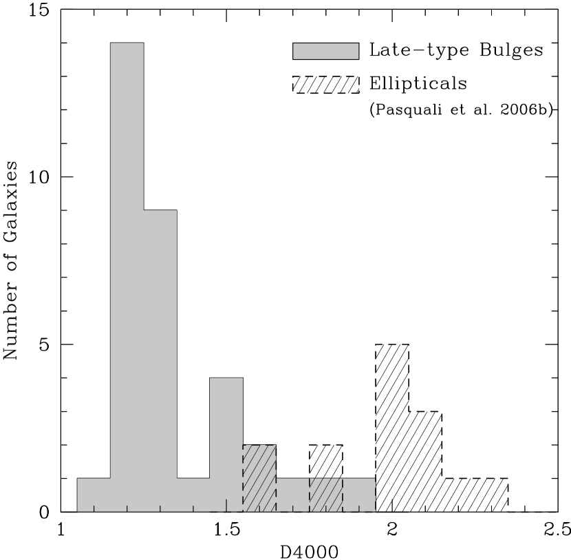
Figure 1.— Distribution of amplitude of 4000 Å  break (D4000; Balogh et al., 1999) for all galaxies in our sample (grey histogram). D4000 was measured as a ratio of average continuum flux redward and blueward of the 4000 Å break from 1D GRAPES grism spectra. The average value of the D4000 for our sample is $\sim$1.3 and for comparison, elliptical galaxies have D4000 $>$ 1.6 (Kauffmann et al., 2003; Padmanabhan et al., 2004). We have also plotted D4000 (hashed histogram) for GRAPES/HUDF early-type galaxies ($0.6\!\leq\!z\!\leq\!1.1$). (Pasquali et al., 2006b).

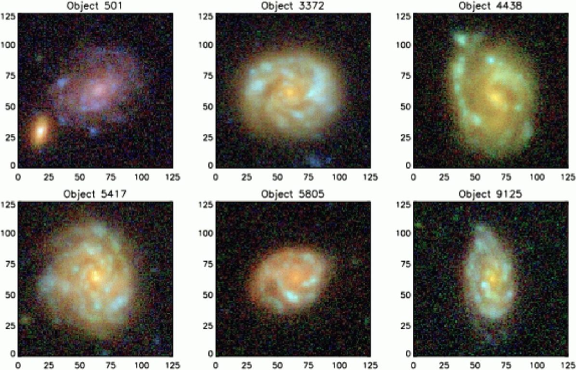
Figure 2.— Color composite images of a representative sample of late-type spiral galaxies at $z\!\simeq\!1$. Axes show size of the stamp in pixels (0.03″/pixel). Note that all have small central bulges that are (in general) redder than their disks.

Table 1 shows the optical ($BVi^{\prime}z^{\prime}$) magnitudes, the HUDF IDs, and coordinates for each selected galaxy, as obtained from the published HUDF catalog (Beckwith et al., 2006). The last column of Table 1 gives the observed ($V$–$z^{\prime}$) colors for these galaxies, corresponding to roughly rest-frame ($U$–$B$) colors at $z\!\simeq\!1$. Table 2 gives all available redshifts for these galaxies. The first 3 columns in Table 2 show the published HUDF IDs and coordinates, while the fourth column shows the photometric redshifts from the GRAPES spectro-photometric redshift catalog (for description, see Ryan et al., 2007) or the GOODS-MUSIC (MUltiwavelength Southern Infrared Catalog) catalog (Grazian et al., 2006). The fifth column of Table 2 gives the spectroscopic redshifts from VLT (Grazian et al., 2006; Vanzella et al., 2008), when available. The last column of Table 2 gives the redshifts from GRAPES SED fitting as described in § 4. The latter are the redshifts used throughout this paper. Notice that estimating the redshift of faint spectra without emission lines can be challenging even for deep surveys such as VVDS (Le Fèvre et al., 2005). Our slitless grism data have an optimal spectral resolution that maximises the S/N for populations with a prominent 4000 Å break. Comparisons of redshift estimates of faint ($i_{\rm AB}\!\simeq$22–24 mag) early-type galaxies at $z\!\simeq\!1$ from the Probing Evolution And Reionization Spectroscopically (PEARS) survey show that ACS slitless grism data often fare better than publicly available spectroscopic redshifts (Ferreras et al. 2008, in preparation).

2.3. Observed Color Profiles

We used the Interactive Data Language (IDL) procedure APER to compute aperture photometry using several aperture radii. We chose our starting aperture radius to be 2.5 ACS pixels ($\sim$0$\farcs$1), because the width of the narrow extraction window (see Pirzkal et al., 2004, for extraction details) of our GRAPES spectra is 5 pixels. We measured aperture magnitudes for all galaxies in our sample in all four ACS bands ($BVi^{\prime}z^{\prime}$) available from the HUDF with aperture radii ranging from 2.5 pixels to 35 pixels. Using these aperture magnitudes, we measured the ($V$–$z^{\prime}$) color profiles for our galaxies. Figure 3 shows these color profiles for 6 sample galaxies. This figure show that the inner disk in most of these galaxies is red, and is dominated by the older stellar population. Our galaxies show that for all apertures the ($V$–$z^{\prime}$) color is redder than 0.9, with redder colors at smaller aperture sizes (the central bulge region).

Figure 3.— Observed ($V$–$z^{\prime}$) colors measured using aperture magnitudes in eight different size apertures. Here we show colors for six sample galaxies. These are the same six galaxies shown in Figure 2. Note that with the exception of object ID 501, all these galaxies become bluer from the inside outwards.

Figure 4 shows the observed ($V$–$i^{\prime}$) color as function of redshift for bulges and spheroids. The black dots correspond to our sample of HUDF/GRAPES bulges. The crosses are the GOODS/HDF-N spheroids presented by MacArthur et al. (2008), and the filled triangles are the GOODS/CDF-S early-type galaxies from Ferreras et al. (2005). The lines represent the expected color evolution for a set of star formation histories using the population synthesis models of Bruzual & Charlot (2003). The thick lines track the color evolution for a stellar population with solar metallicity and an exponentially decaying star-formation rate, starting at z${}_{F}=5$, with an exponential decay timescale of 0.5 (solid), 1 (dashed) and 8 Gyr (dotted). The thin solid line shows the expected color evolution for a decay timescale of 0.5 Gyr and 1/3 of solar metallicity. Most of the bulges in early-type galaxies in GOODS/CDF-S (Ferreras et al., 2005; MacArthur et al., 2008) are consistent with short decay timescales, while the bulges in our late-type spiral sample agree better with a more extended star formation history. This figure shows that the bulges explored in this paper belong to a similar population as the “blue early-types” presented in Ferreras et al. (2005). This blue population constitutes $\sim$20% of the total sample of early-type systems visually selected in GOODS/CDF-S. Because of the excellent photometric depth of the HUDF, our sample extends the bulge redshift distribution of MacArthur et al. (2008) to $z\simeq 1.3$.

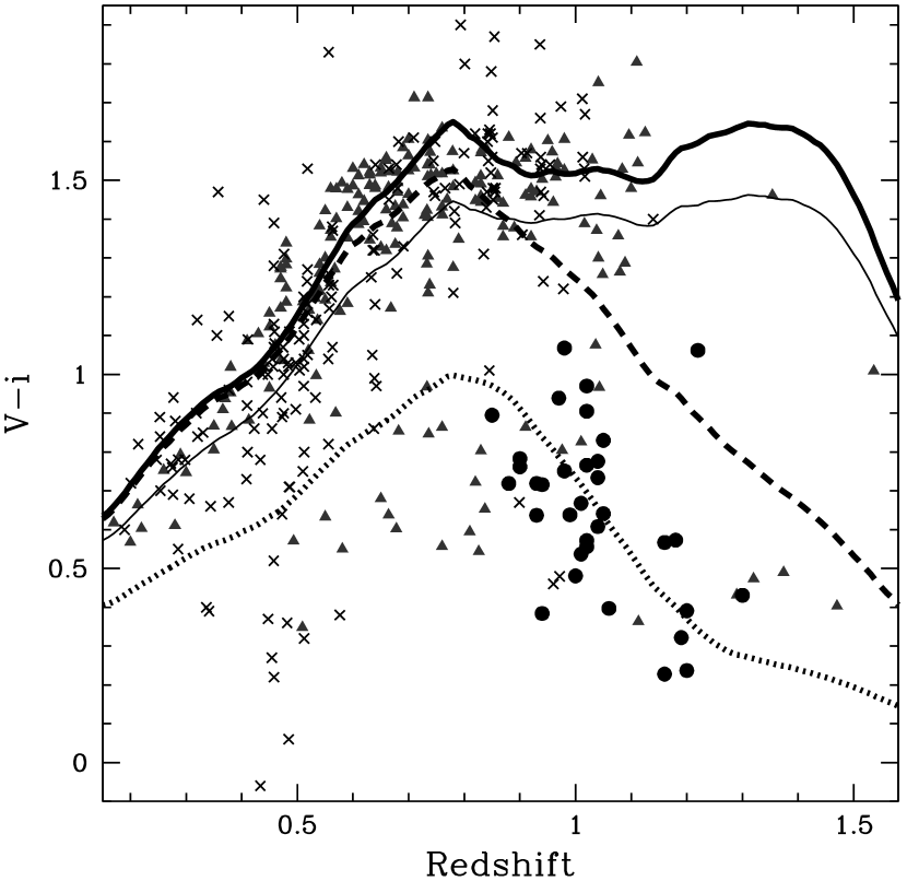
Figure 4.— Color vs. redshift diagram of bulges and spheroids. The black dots correspond to our sample of HUDF/GRAPES bulges. The crosses are the GOODS/HDF-N spheroids presented by MacArthur et al. (2008), and the triangles are the GOODS/CDF-S early-type galaxies from Ferreras et al. (2005). The lines represent the expected color evolution for a set of star-formation histories from the population synthesis models of Bruzual & Charlot (2003). The thick lines track the color evolution of a stellar population with solar metallicity and an exponentially decaying star-formation rate starting at z${}_{F}=5$, with an exponential decay timescale of 0.5 (solid), 1 (dashed) and 8 Gyr (dotted). The thin solid line shows the evolution with a timescale of 0.5 Gyr at 1/3 of solar metallicity.

3. Morphological Properties

We performed a morphological analysis of the sample galaxies in two steps: (a) a non-parametric analysis of the distribution of the galaxy light, using the measures of asymmetry, concentration and clumpiness (or smoothness) to confirm our visual inspection; (b) a two dimensional (2D) decomposition performed with GALFIT (Peng et al., 2002), in order to quantify the galaxy morphology and in particular to extract their Sérsic indices.

3.1. CAS Measurements

We use the classical Concentration (C), Asymmetry (A) and clumpinesS (or smoothness) — the CAS parameters (Conselice et al., 2000; Conselice, 2003) — to carry out the non-parametric approach to quantify morphology. We computed the C and A values for our galaxies following the definitions and methods as discussed in Conselice et al. (2000). The Concentration index correlates with the Sérsic index and the Bulge-to-Disk ratio: high C-values correspond to early-type morphology, while lower C-values are suggestive of a disk-dominated or later-type and irregular galaxies. Asymmetry can distinguish irregular galaxies or perturbed spirals from relaxed systems, such as E/S0 and normal spirals. Clumpiness quantifies the degree of structure on small scale, and roughly correlates with the rate of star-formation. We derived the Concentration and Asymmetry indices using the images taken in the $z^{\prime}$-band, which roughly corresponds to the rest-frame $B$-band at $z\!\simeq\!1$. Our measurements of C and A are shown in Figure 5, together with the mean loci for nearby early-, mid- and late-type galaxies as derived by Bershady et al. (2000). A few perturbed galaxies show higher asymmetry values. Figure 5 clearly shows that our sample of galaxies consists of mostly late-type galaxies, and confirms our visual morphological classification of late-type galaxies with bulges.

Figure 5.— Asymmetry and Concentration values for the selected late-type galaxies. The distinction between early-, mid- and late-type galaxies is from Bershady et al. (2000) and Conselice et al. (2005). According to this classification scheme, our sample – selected by the presence of a prominent 4000 Å  break and removing the spheroidal galaxies – corresponds to late-type spirals.

3.2. 2D Galaxy Fitting using GALFIT

GALFIT (Peng et al., 2002) is an automated algorithm to extract structural parameters from galaxy images by fitting/decomposing these with one or more analytic 2D functions. It offers different parametric models (the “Nuker” law, the generalized Sérsic–de Vaucouleurs profile, the exponential disk, and Gaussian or Moffat functions), and allows multi-component fitting, which is useful to measure Bulge-to-Disk (B/D) or Bulge-to-Total (B/T) light ratios.

3.2.1 Thumbnail Image Extraction

The GALFIT disk+bulge decompositions were performed on thumbnail (or “postage stamp”) images extracted around the objects in our sample, rather than on the entire science image itself. Three thumbnail images for each object were extracted from the original HUDF images. All thumbnail images are 201$\times$201 pixels ($\sim$ 6$\farcs$0$\times$6$\farcs$0) in size. The first thumbnail was extracted from the science image itself. The second thumbnail was extracted from the comprehensive segmentation image generated by Coe et al. (2006), which was used as the “bad pixel map/mask” image used in GALFIT. GALFIT uses this “mask” image so that all non-zero valued pixels are ignored in the fit. Hence, the extracted segmentation stamps were modified, so that only pixels belonging to the galaxy had zero value, while any pixels belonging to another object are set to a non-zero value. We tested this GALFIT decomposition with and without bad pixel maps for comparison, and obtained very similar fitting results. The third thumbnail was extracted from the drizzle-generated weight image (Koekemoer et al., 2002). These weight images were modified for GALFIT (C. Peng, private communication) as follows. First, the science image was smoothed by a few pixels to get rid of some of the random pixel-to-pixel variations. Second, a variance image $S$, was calculated using $S=(1/wht)+data/exptime$, where, $wht$ is the drizzle-generated weight image, $data$ is the science image in counts/sec and $exptime$ is the total exposure time of the image. Finally, a sigma image is generated using $\sigma=\sqrt{S}$. These modified weight images were used as the input “sigma” image (noise maps) in the GALFIT, which is necessary for proper error-propagation.

3.2.2 Sky Background

The drizzled HUDF images are sky subtracted and therefore, to understand the effects of sky-subtraction, we used the following procedure. A careful analysis of the HUDF sky-background and its corresponding uncertainties was performed by Hathi et al. (2008b). We used the sky-background values from Hathi et al. (2008b), and allowed GALFIT to either vary this sky-level during the fitting process, or keep it fixed. For comparison, we also used the sky-background measured from each individual object stamp, and repeated the process. We also tested our GALFIT decomposition by comparing the results from GALFIT with and without the addition of the sky-background. We found very consistent and similar fitting parameters from all these tests. Therefore, we adopted the sky-background levels measured by Hathi et al. (2008b) in our final GALFIT decomposition.

3.2.3 Using GALFIT

GALFIT produces model images of galaxies based on initial input parameters. These images are convolved with the ACS Point Spread Function (PSF) image before comparing with the actual galaxy image. Fitting proceeds iteratively until convergence is achieved, which normally occurs when the $\chi^{2}$ does not change by more than 5 parts in 10⁴ for successive five iterations (see Peng et al., 2002, for details).

GALFIT requires initial guesses for the fitting parameters. Following Dong & De Robertis (2006) and Simien & de Vaucouleurs (1986), we used the output parameters from the published HUDF SExtractor catalogs (Beckwith et al., 2006) as input values for the magnitude, the half-light radius, the position angle, and the ellipticity of each object. The initial value for the Sérsic index, $n$, was taken to be 1.5 (Coe et al., 2006). Tests based on an adopted initial value of $n$=4 showed similar results.

All GALFIT measurements were obtained from the $V$- and $z^{\prime}$-band images (approximately rest-frame $U$- and $B$-band at $z\!\simeq\!1$, respectively). First, we fitted only an one-component Sérsic profile to our galaxies to improve the initial estimates for the Sérsic  index, the axis ratio and the position angle of each galaxy. The distribution of Sérsic indices for our galaxies in the $V$- and $z^{\prime}$-band is shown in Figure 6. Our measurements of the Sérsic index in $V$- and $z^{\prime}$-band are comparable to $i^{\prime}$-band values of the galaxies in Coe et al. (2006). Figure 6 confirms that most of the galaxies in our sample have a Sérsic index $n<2$ in both $V$- and $z^{\prime}$-bands, which implies that our galaxies are disk-dominated, as Figure 2 and Figure 3 clearly suggest.

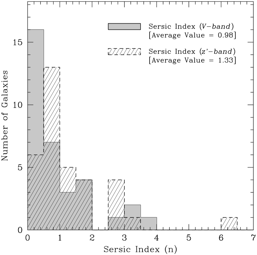
Figure 6.— The distribution of Sérsic indices ($n$) for the galaxy retrieved from GALFIT single component Sérsic fit to galaxies in $V$- and $z^{\prime}$-band. The mean values of $n$ is reported in top right corner. Using a two-sided K-S test on these distributions, we cannot reject the hypothesis that the $V$- and $z^{\prime}$-band distributions are drawn from the same population.

Next, we simultaneously fitted two components: a Sérsic profile plus an exponential disk profile, to get better estimates of the bulge and disk magnitudes, respectively. For this simultaneous fit, we kept the coordinates of the galactic center (within $\pm$1 pixel constraint), the axial ratio and the position angle fixed, while we allowed GALFIT to fit $m_{bulge}$, $m_{disk}$, $R_{e}$, $R_{s}$ and the the Sérsic index ($n$). For all galaxies in our sample, we obtained better fits for bulge Sérsic indices of $n\lesssim 1.0$. We also tested our runs by fixing initial value of $n$=1 for all galaxies and found that GALFIT converged to similar solutions in the end. The bulge and disk models obtained from these best fits were then used to estimate the B/D ratio. We used an aperture of 5 pixels diameter to measure the B/D and B/T ratios, which used the same aperture size as for extracting the GRAPES SEDs. The majority of our galaxies show a B/D value $<$1 within this aperture. For larger apertures encompassing the galaxies’ total light, B/D appears to be $<<$ 1, in agreement with our galaxies being disk-dominated (i.e., late-type galaxies).

4. Stellar Population Models - Bulge Properties

The GRAPES grism spectra were taken at five different position angles (PAs) to remove any contamination and overlap from nearby objects. We generated one final spectrum for each galaxy by combining all of the GRAPES spectra obtained at the 5 different PAs. The combination was performed as a simple averaging operation, after resampling the spectra onto a common wavelength grid. Portions of spectra which were contaminated more than 25% (see Pirzkal et al., 2004, for a description) were not used, unless absolutely necessary. The Poisson errors were propagated, and the standard deviation of the mean between the 5 individual PAs was computed. The larger of either the Poisson noise or the standard deviation of the mean was used in the subsequent analysis. Our goal is to fit stellar population models to the age-sensitive 4000 Å break observed in the GRAPES spectra of these galaxies.

4.1. Star-Formation Histories (SFH)

We fit our ACS grism spectra to a grid of models obtained by combining the simple stellar populations of Bruzual & Charlot (2003). A standard $\chi^{2}$ method is used. We explore a wide volume of parameter space in order to infer robust constraints on the possible ages and metallicities of the stellar populations in the central bulges of these galaxies. This comparison requires a careful process of degrading the synthetic SED (resolution $R\sim 2000$) to the (variable) resolution of the GRAPES spectra. Special care must be taken with respect to the change of the Line Spread Function (LSF) with wavelength, which results in both an effective degradation of the spectral resolution as a function of wavelength, and a different net spectral resolution with respect to the size of the galaxy. After exploring a range of values $R\!=30-80$, we find that an effective resolution of $R=50$ is suitable for all the spectra in our sample. The ACS grism spectral resolution is not degenerate with respect to parameters describing the star-formation history, and mostly results in a global shift of the likelihood.

In order to determine the redshift as accurately as possible, we start with some guessing values obtained from three sources: a photometric redshift; a VLT spectroscopic redshift — where available — and a redshift estimate taken from an automated method (as discussed in § 2.2) to search for a prominent 4000 Å  break in GRAPES data. A small set of templates at the GRAPES resolution were used to determine the best redshift for each galaxy, using the guessing values described above as a starting point, and performing a simple cross-correlation for a range of redshifts until the best match is found. This method generates the redshifts used throughout this paper, shown in Table 2 as “SED Fit” (last column).

In order to make a robust assessment of the ages and metallicities of the unresolved stellar populations, we use two different sets of models to describe the build up of the stellar component. The models depend on a reduced set of parameters, which can characterize a star-formation history in a generic way.

Model #1 (EXP): We take a simple exponentially decaying star formation rate, so that each star-formation history is well parametrized by a formation epoch, which can be described by a formation epoch ($t(z_{F})$); a star-formation timescale ($\tau_{\star}=0.1\rightarrow 4$ Gyr); and a metallicity ($[m/H]=-1.5\rightarrow+0.3$), which is kept fixed at all times. The numbers in brackets give the range explored in the analysis of the model likelihood. The range in formation epochs is chosen from $z_{F}=10$ to $t(z_{F})=0.2$ Gyr (this range depends on the observed redshift of the galaxy).

Model #2 (CSP): We follow a consistent chemical enrichment code as described in Ferreras & Silk (2000). The model allows for gas infall and outflow. The metallicity evolves according to these parameters, using the stellar yields from Thielemann et al. (1996) for massive stars ($>10M_{\odot}$), and van den Hoek & Groenewegen (1997) for intermediate mass stars. The free parameters are the formation epoch (same range as the one chosen for Model #1), the timescale for the infall of gas ($\tau_{f}=0.1\rightarrow 1$ Gyr), and the fraction of gas ejected in outflows ($B_{\rm OUT}=0\rightarrow 1$). The star-formation efficiency is kept at a high value $C_{\rm EFF}=20$ as expected for early-type populations (see Ferreras & Silk, 2000).

For each of the two sets of models we run a grid of SFHs, convolving simple stellar populations from the models of Bruzual & Charlot (2003). The grid spans $64\times 64\times 64$ SFHs (note that three free parameters are chosen in each set) over a wide range of values as shown above. Once the best fit is obtained within the grid, we run a number of models with random values of the parameters with an accept/reject criterion based on the likelihood – analogous to the Metropolis algorithm, e.g., Saha (2003). The process ends when 10,000 models are accepted. The total number of accepted models determine the median and confidence levels of the parameters. The distribution of reduced $\chi^{2}$ values has an average of $\chi^{2}$=0.74 and RMS $\sigma(\chi^{2})=0.35$. The $\chi^{2}$ used throughout includes a mild Gaussian prior on the metallicity with average [m/H]$=-0.1$ and RMS $\sigma([m/H])=0.5$. This prior allows for a relatively wide range of average metallicities, and is compatible with the values commonly found in these systems (e.g., Carollo et al., 2007). For the interested reader, we include an appendix describing in detail the effect of the application of this prior. We find no significant change in the estimates of the stellar age distribution with or without priors.

Figure 7 shows the best fit models and the observed SEDs for 10 galaxies in our sample. The error bars represent the observations, and the solid line corresponds to the best fits for the CSP model. The wavelength is shown in the observed frame, whereas the wavelength range chosen for all galaxies is 3800–5000 Å in the rest-frame. This choice ensures a consistency in the comparison of the stellar populations in our sample. The chosen range straddles the age-sensitive 4000 Å  break. To illustrate the uncertainties of estimating stellar ages within the modelling, we show in Figure 8 the likelihood distribution with respect to average stellar age for each galaxy.

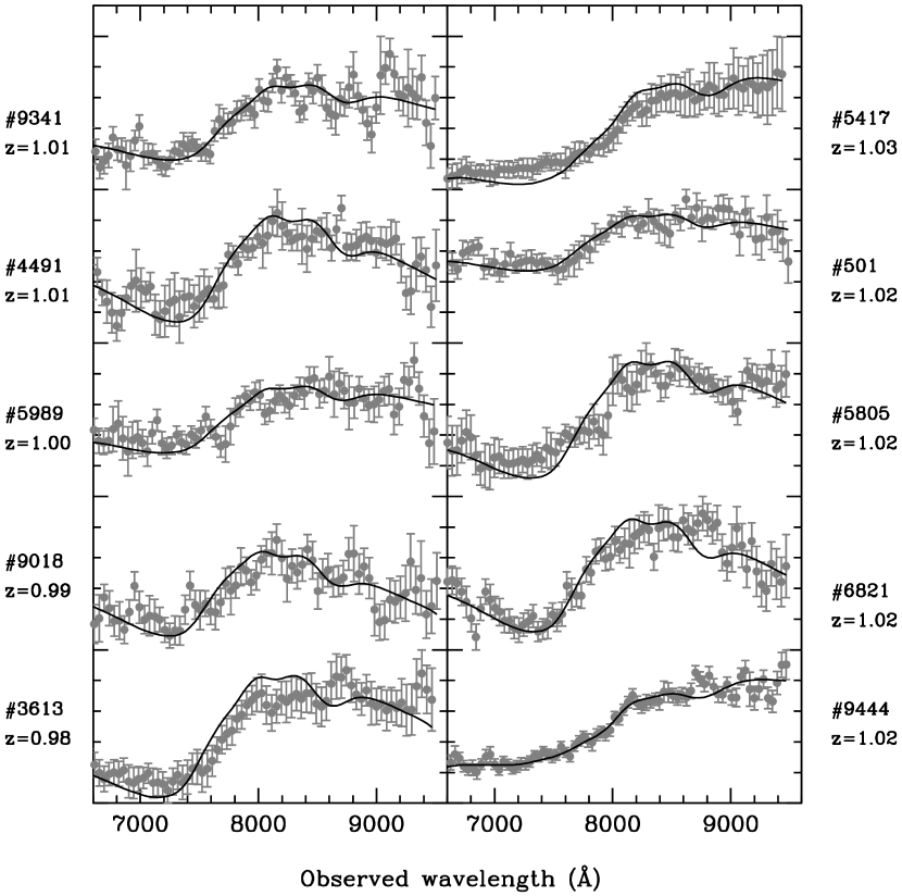
Figure 7.— Spectral energy distributions of 10 galaxies in our sample (each one is labeled with the HUDF numbers and model redshifts). The error bars are the observed ACS/G800L data and the lines are the best fits according to the CSP models (see text for details). The distribution of reduced $\chi^{2}$ values for all galaxies in our sample has an average of $\chi^{2}$=0.74 and RMS $\sigma(\chi^{2})=0.35$.

Figure 8.— The likelihood distribution with respect to average age for all 34 bulges.

Figure 9 shows the 4000 Å  break amplitude, D4000, as a function of stellar age. The distribution of bulge ages is overplotted as a histogram, which agrees very well with the observed range in D4000 – which is 1.2 to 1.5, as shown in Figure 1. Different curves show three simple stellar population models with three different metallicities. For metallicity around solar (thick-solid and dashed lines), representative of our bulges, the variation in D4000 with age is very similar. For solar metallicity with E($B$–$V$)=0.2 dust reddening (thin-solid line) and for high metallicity (dotted line), the relation is somewhat steeper. Figure 9 shows that for the range in D4000 and metallicities of our sample, the effect of metallicity on D4000 is small, hence D4000 is a good age indicator for this sample.

Figure 9.— The 4000 Å  break amplitude, D4000, as a function of stellar age. The distribution of bulge ages is overplotted as histogram, which agrees very well with the range in D4000 (see Figure 1). Different curves show three simple stellar populations model with three different metallicities, as labelled. The effect of dust on a solar metallicity model is shown as a thin solid line. The figure illustrates that for the range of ages found in our sample, the degeneracy caused by dust and metallicity will not result in a significant change of the average stellar ages. Furthermore, if the bulges were dusty or more metal rich, the resulting populations would become even younger, ruling out the possibility of bulges as old as early-type galaxies at the same redshift.

Figure 10 shows the ages and metallicities of the best SFHs for each bulge. The average and RMS scatter for age and metallicity are shown as dots and error bars, respectively. For the EXP models – which have zero spread in metallicity – the error bars in metallicity represent the uncertainty estimated from the likelihood. The solid lines in the lower panels correspond to the age of the Universe as a function of redshift. The dashed lines show the age that a simple stellar population – a population with a single age – would have if formed at redshifts (from top to bottom) $z_{F}\!=\!\{5,3,2\}$. The median value of the stellar ages of our bulges is 1.3 Gyr. The CSP models treat chemical enrichment in a more consistent way than the EXP models and should therefore better reflect the true populations. We use mass-weighted average ages for these stellar populations from the SFHs because they better reflect the formation process of bulges (or galaxies in general). A very small amount of young stars – something that may not reflect the true formation process of the bulge – can have a large effect on luminosity-weighted ages. By using composite models such as EXP or CSP we minimise this contamination by using the mass-weighted ages instead.

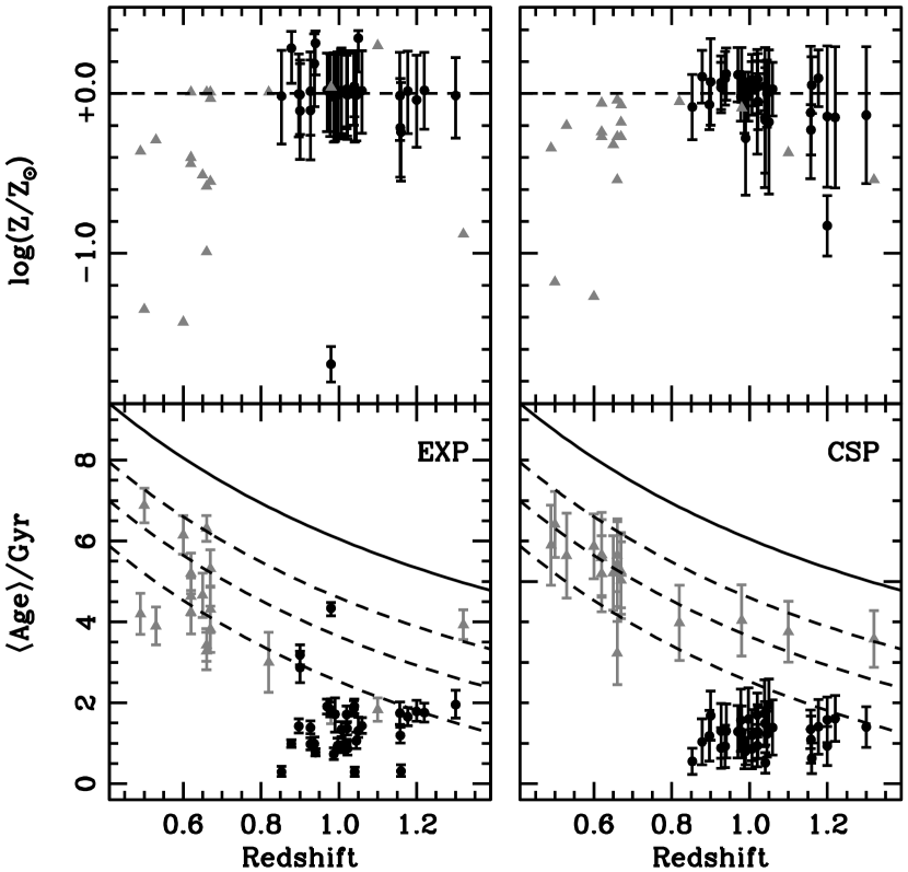
Figure 10.— Ages and metallicities corresponding to the best fit according to a simple exponentially decaying model (EXP; [Left]) or a consistent chemical enrichment code (CSP; [Right]). The filled circles are the average values of age or metallicity and the error bars represent the RMS of the distribution. The solid lines in the bottom panel track the age of the Universe at a given redshift for a concordance cosmology. The dashed lines – from top to bottom – correspond to the ages that simple stellar populations would have if formed at redshifts $z_{F}=\{5,3,2\}$. The grey triangles are the GRAPES/HUDF early-type galaxies from Pasquali et al. (2006b), whose SEDs were analyzed the same way as in this paper.

We would emphasize here that it is the average stellar age that can be reasonably constrained with the data. Therefore, Figure 10 does not imply that all stars in these bulges are $\sim$1.3 Gyr but many may be older. To clarify, the formation epoch (characterized by a formation redshift) is the age when star formation starts in the model. Comparing observations and models of unresolved stellar populations can only give us robust average ages (the first order moment of the age distribution) and, with higher uncertainty, we can also determine the “width” of the age distribution (the second order moment). We caution the reader that the actual parameters used in the modelling (especially formation redshift) constitute a way to characterise a generic set of star formation histories, but the uncertainties in these parameters will be larger than those in the average age, which we consider to be the main physical property that can be extracted from the data. We would also clarify here that we have used ‘Age’ or ‘<Age>’ in various figures showing age distributions. When figures are based on single stellar population models we use ‘Age’, and when figures are based on composite models (EXP, CSP) we use ‘<Age>’, as they cannot give a single age by definition.

4.2. Bulge Mass Estimates

The photometry from Table 1 can be combined with the M/L ratios obtained from the best-fit SFH to constrain the stellar mass (M_s) content of the bulges. This M/L is derived from the composite model obtained by combining the simple stellar populations from Bruzual & Charlot (2003) using a Chabrier (2003) Initial Mass Function (IMF). If we change the IMF from Chabrier (2003) to Salpeter (1955), the stellar mass will increase by $\sim$0.3 dex in $\log$(M_s), which within the other errors in data and models, does not change our overall results. The photometry has to be corrected to take into account contamination from the disk, as we discuss in § 4.3. We use the B/D ratio obtained from the GALFIT (§ 3.2) to estimate the bulge fraction of the light in the galaxy. The stellar mass estimates for our bulges are in the range of $6.5\!\leq\!\log($M${}_{s}/$M${}_{\odot})\!\leq\!10.0$.

Figure 11 shows the predicted average and RMS of the age distribution as a function of stellar mass and redshift. Over the stellar masses and redshifts probed in this sample we find a similar average age and scatter. This similarity could be due to two possible reasons. First, our sample spans a redshift range from $z\!\simeq\!0.8$ to $1.3$, corresponding to a difference in lookback time of $\sim 1.9$ Gyr. This is comparable both to the uncertainty in the age estimate and to the RMS of the distribution. Secondly, Vanzella et al. (2006) found Large Scale Structure (LSS) in the CDF-S around $z\!\simeq\!1.0$ from VLT spectroscopic redshifts. The redshift distribution in the HUDF (smaller field in the CDF-S) also show a strong peak around $z\!\simeq\!1.0$. So it is possible that we may be looking at a smaller subset of this LSS at $z\!\simeq\!1.0$.

Figure 11.— The average age [Bottom] and RMS scatter [Top] of the age distribution is shown with respect to stellar mass (left) and redshift (right). Typical error bars are shown. The lookback time difference between redshifts $z=0.8$ and $1.3$ is $1.9$ Gyr, i.e., comparable to the scatter in average ages, which explains the lack of a trend of average age with redshift.

4.3. Disk Contamination in the GRAPES Grism Spectra

The best-fit stellar population models to the GRAPES SEDs suggests that the late-type bulges at $z\!\simeq\!1$  are young, with an average age of $\sim$1.3 Gyr. To better understand this result, we first need to quantify the effect of disk contamination in our measurements. The GRAPES SEDS are extracted from an aperture of relatively narrow-width aperture (5 pixels in diameter) around the center of each galaxy. The narrow extraction of the grism spectra is dominated by the bulge and the inner disk light; since we use its 4000 Å break to date the bulge, we need to investigate the spectral contamination due to inner disk on the estimated bulge age. We perform following photometric tests to understand the effect of the inner disk on the bulge ages.

(1) We used the disk and bulge light profiles produced by GALFIT and measured their flux in a strip 5 pixel wide and around their common center, to estimate the disk and bulge light-fraction within this aperture. We find that the light contributed by the disk to the total flux in this aperture can be as high as 30%. At the same time, we measured the disk and bulge colors within the same aperture, to find that the disk and the bulge are similar within the photometric errors, so that the disk contamination in the bulge spectrum is not expected to dominate our estimate of the bulge age (see Appendix B for further discussion). This can be already be seen in Figure 3, where the bulge is in general 0.3–0.8 mag redder in ($V$–$z^{\prime}$) than the disk.

(2) We compared the bulge age derived from the stellar population models with the color difference between two apertures. We measure the color difference between two apertures with 2.5 pixels and 5 pixels radii, equivalent to the narrow and wide GRAPES spectral extractions, respectively. The top panel of Figure 12 shows the comparison between the color difference and the bulge age. The points on the plot are color-coded according to their B/D ratios, measured from GALFIT as discussed in § 3.2. Blue color stands for B/D$\leq$0.5, green means 0.5$<$B/D$\leq$1 and red represents B/D$>$1. The top panel of the Figure 12 does not show any major trends among age, color difference, and B/D ratio. Secondly, we compared the bulge age to the color difference between the 2.5 pixels aperture and the annulus defined by the 2.5 and 5 pixels apertures. The bottom panel of the Figure 12 shows this comparison. The points on the plot are color-coded according to their B/D ratios, as in the top panel. Like the top panel, the bottom panel of Figure 12 does not show any major correlation among age, color difference, and B/D ratio. Finally, we directly compared the B/D ratio with the age and mass of the bulge. The top panel of Figure 13 shows the comparison between the B/D ratios obtained from the GALFIT and the bulge age from the stellar population models for all galaxies in the sample. Figure 13 does not show any correlation between the age and the B/D ratio. Similarly, the bottom panel of Figure 13 shows at best a very mild correlation between the bulge stellar mass and the B/D ratio.

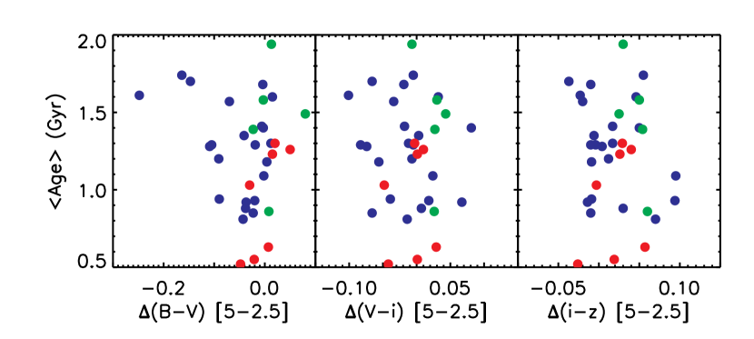
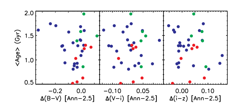
Figure 12.— Comparison between aperture colors and the best-fit bulge age. [Top] shows the bulge age as a function of the color difference between the 2.5 pixels aperture and the 5 pixels aperture. [Bottom] shows the bulge age as a function of the color difference between the 2.5 pixels aperture and the annulus defined by the 2.5 and 5 pixels apertures. A blue colored circle stands for B/D$\leq$0.5, green means 0.5$<$B/D$\leq$1 and red represents B/D$>$1. Here B/D is measured in the $i^{\prime}$-band as discussed in § 3.2. Both panels does not show any correlation among the age, color difference, and B/D ratio.

Figure 13.— The Bulge-to-Disk (B/D) ratio measured with GALFIT is compared with average age [Top] and stellar mass [Bottom]. Similar to the trend in Figure 11, average age does not correlate with B/D either. However, the bottom panel suggests a correlation with stellar mass.

(3) For a few sample galaxies, we extracted the spectrum of their disk above and below the bulge aperture used to extract the bulge spectrum, at a distance of approximately 10 pixels from the galaxy center. Similarly to its bulge, the inner disk also exhibits a 4000 Å break in the spectrum whose amplitude is only slightly smaller (within few percents) than the bulge. This test shows that both bulges and inner disks are equally red/old, as expected from an inside-out formation scenario. We also fitted stellar population models using both the bulge and disk spectra, and analyzed how the bulge-age and metallicity change as a function of disk contamination, i.e., the fraction of disk light added to the bulge spectrum. Our simulations (discussed in Appendix B) show that the determination of the bulge age is not dominated by disk contamination. Even when disk contamination is completely ignored – or fully subtracted – the bulge ages do not change much.

In summary, we do not detect any significant correlation between the bulge age, B/D ratio and the aperture color difference. We thus conclude that our estimate of the bulge ages is fairly robust, and that the younger age of the sample bulges is likely real and not due to disk contamination.

5. Discussion

The ages and masses of late-type bulges are estimated by fitting our GRAPES SEDs with stellar population models. Our analysis shows that bulges in late-type galaxies at higher redshift ($z\!\simeq\!1$) appear to be relatively young, with an average age $\sim$1.3 Gyr ($6.5\!\leq\!\log($M${}_{s}/$M${}_{\odot})\!\leq\!10.0$) compared to early-type galaxies at the same redshift. This finding appears to be independent of the relative amount of disk-light present, or the color of the underlying disk.

Figure 14 shows the stellar masses of our bulges (filled and open circles) compared with the best-fit average ages from the CSP models discussed in § 4. We also include the sample of early-type galaxies from GRAPES/HUDF (grey triangles; Pasquali et al., 2006b), whose GRAPES spectra were analyzed in a similar way. The early-types sample covers a wider range of redshifts ($0.5\leq z\leq 1.1$). Hence, for a proper comparison, we divide both bulges and early-type galaxies with respect to redshift roughly about the median value for each subsample $z\sim 1$ for bulges and $z\sim 0.65$ for early-types. The solid (hollow) symbols correspond to the lower (higher) redshift bin, respectively. The bulges in our late-type spirals span a much lower range of ages, and, obviously, have lower stellar masses, compared to those of early-type galaxies.

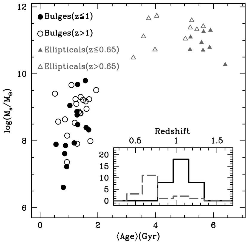
Figure 14.— Comparison between the ages of the bulges in this sample (black circles/lines) and early-type galaxies in GRAPES/HUDF (grey triangles/dashed lines; Pasquali et al., 2006b). The inset shows the histogram of redshifts for both samples with ellipticals peaking around $z\!\simeq\!0.65$. Both samples are split with respect to redshift, with solid symbols representing the lower redshift subsample. There is a very significant difference between the average age of early-type galaxies and galaxy bulges. Furthermore, the age difference is better defined for early-types, suggesting passive evolution for these galaxies and a more extended star formation history for the bulges.

Elmegreen et al. (2005) have classified $\sim$900 galaxies (larger than 10 pixels or 0.3″) in the HUDF according to morphology and their photometric properties. They find 269 spiral galaxies in the HUDF. Using the Elmegreen et al. (2005) morphological classifications, and accurate spectro-photometric redshifts from Ryan et al. (2007), we estimate that the results in this paper represent approximately $\sim$40–50% of the total late-type/spirals HUDF galaxy population within the magnitude and redshift range used in this paper.

Our analysis of the central and the inner disk colors of these galaxies (Figure 3) and their grism spectra (as discussed in the Appendix B) shows that the inner disk and the bulge components have similar colors, and that the bulge ages are not significantly affected by the light (and stellar populations) of the underlying disk. This result is consistent with the idea that the inner disk of galaxies in general has similar colors and age as the bulge (e.g., Peletier & Balcells, 1996). The effect of dust on these measurements should not be significant, since our bulge ages are based on the amplitude of the 4000 Å observed in the GRAPES grism spectra, which is mostly sensitive to age and has a weak dependence on dust (see Figure 9). Also, MacArthur et al. (2004) argue that dust is generally not a significant contributor to galaxy colors in low-mass/low-luminosity spiral galaxies, but is likely important in more massive/brighter galaxies. On the other hand, even if it plays an important role in this analysis, the inclusion of dust will make our ages even younger, and our result that bulges and inner-disks have similar dominant stellar population with an average age of $\sim$1.3 Gyr should then be viewed as an upper limit.

We performed GALFIT decomposition on the sample galaxies by simultaneously fitting the bulge to a Sérsic profile and the disk to an exponential profile. For all bulges in our sample, we obtained better fits using Sérsic  indices of $n\lesssim 1.0$. Therefore, these bulges are disk-like (Kormendy & Kennicutt, 2004; Athanassoula, 2005) and have radial surface brightness profiles similar to disks. Similar analyses for local spirals by de Jong (1996) and Courteau et al. (1996) have shown that the majority of bulges in late-type galaxies are better fit by exponential profile. Our results show that a similar trend also exists at $z\!\simeq\!1$. The similarities we find in the bulge and the inner-disk properties (4000 Å  break, colors and profiles) could imply that these less massive, younger bulges at $z\!\simeq\!1$  grow through secular evolution processes (Kormendy & Kennicutt, 2004). At $z\!\simeq\!1$, it is possible that we are seeing these galaxies still forming, and these “disk-like” bulges might grow from disk material or minor mergers to become more massive bulges observed at present day. Disk-like pseudo-bulges can also grow by gas inflow and star-formation. Bars can drive central gas inflows (Sheth et al., 2005), and therefore, there could be a correlation between these disky bulges and central bars. Sheth et al. (2008) find that the bar fraction in very massive, luminous spirals is constant from $z\!\simeq\!0$ to $z\!\simeq\!0.84$, whereas for low-mass, blue spirals it declines significantly with redshift to about $\sim$20% at $z\sim 0.84$, indicating that some bars do form early enough. Elmegreen et al. (2005) has morphologically classified few ($\sim$10%) of our sample galaxies as barred galaxies, so it will be interesting to investigate these late-type galaxies in future studies to understand this relation.

Aperture color analysis by Ellis et al. (2001) for bulges at $z\!\lesssim\!0.6$ in early-type and spiral galaxies with $I_{AB}<24$ mag found that their central colors are redder than the surrounding outer disk colors, but that these central colors are bluer than those of pure ellipticals at the same redshifts. As shown in Figure 10, our results agree with Ellis et al. (2001). This is not perhaps surprising, since we also select our sample based on galaxy total-magnitudes, with no constraints on its bulge magnitude. In comparison, Koo et al. (2005) select their sample based on bulge luminosity, and they find that luminous, high-redshift ($0.73\!<\!z\!<\!1.04$) bulges ($I_{AB}<24$ mag) within the Groth Strip Survey are very red/old. They clearly show that if the bulge sample is luminous, then all bulges are equally red and old. In contrast, we show that if the bulge sample is selected without any constraint on the bulge magnitude, then late-type bulges are younger than bulges in early-type galaxies at similar redshifts.

Galaxy colors and structural properties show a bimodal distribution, separating into a red sequence, populated by early-type galaxies, and a blue “cloud”, populated by late-type galaxies (Balogh et al., 2004; Driver et al., 2006). Whether a galaxy resides in a red sequence or a blue cloud is also related to the type of bulge in a galaxy (Drory & Fisher, 2007). Figure 4 shows this bimodal distribution. Our late-type galaxies with pseudo bulges lie in the bluer cloud compared to early-type galaxies that lie on the red color sequence. This shows that the processes involved in the formation of galactic bulges and their host galaxies are very similar. Observations indicate that these formation mechanisms depend strongly on the bulge (as well as galaxy) mass, and that they were active at $z\!\simeq\!1.3$. This evidence is strengthened by the results of Thomas & Davies (2006) and MacArthur et al. (2008), who find that bulges of similar mass have a similar evolutionary path. Possibly because of cosmic variance, we do not detect early-type spirals at $z\!\simeq\!1$ in the HUDF. Comparing our sample of late-type bulges with the massive early-type galaxies at similar redshifts studied by Pasquali et al. (2006b), we confirm the existence of different evolutionary patterns for bulges in early- and late-type galaxies (see Figure 4).

Our analysis of the deepest optical survey, the HUDF, along with the deep unique ACS grism spectroscopy provides the best spatial resolution at $z\!\simeq\!1$, and yields more detailed insight in the process of galaxy formation. Massive and luminous bulges (e.g., Koo et al., 2005), which mostly reside in early-type galaxies and in earlier-type spiral galaxies, are old and formed at $z\!\gtrsim\!2$. The secular evolution suggested by Kormendy & Kennicutt (2004) does not play any role in their formation. Our ACS grism study of the HUDF here has shown that lower-mass bulges, which are mostly associated with later-type galaxies, are on average younger than one would expect by letting their stellar populations passively evolve since their formation redshift $z\!\sim\!2$. This result would point to secular evolution as a likely mechanism to support prolonged star formation in low-mass bulges, which is very different from Pasquali et al. (2006b) ellipticals, for which a quick SFH plus passive evolution can explain their observed SEDs.

6. Summary

We estimated the stellar ages and masses of 34 bulges of late-type galaxies from the HUDF by fitting stellar population models to the 4000 Å break observed in deep ACS GRAPES grism spectra. This study takes advantage of the exceptional angular resolution and depth of the GRAPES/HUDF data, which allow us to identify the small bulge components of this sample of galaxies at $z\!\simeq\!1$, both on the direct and on the grism images, and to extract its corresponding spectrum, a method currently unfeasible with ground-based spectroscopy. We find that bulges in late-type galaxies at higher redshift ($z\!\simeq\!1$) appear to be significantly younger (with an average age of $\sim$1.3 Gyr) than early-type galaxies at similar redshifts. This finding is robust against the amount of disk-light that may contaminate in part the bulge spectrum. The lack of a trend between average age and redshift (see Figure 14) suggests star formation in bulges is extended over much longer times compared to early-type galaxies. Our results support the scenario where low-mass late-type bulges form through secular evolution processes.

Appendix A Effect of Metallicity Priors on Bulge Ages

The modelling of stellar populations in this paper includes a mild prior on the distribution of bulge metallicities. For each choice of a star formation history (characterized by the parameters discussed in § 4) we multiply the likelihood from the $\chi^{2}$ distribution by a Gaussian prior with mean $\log(Z/Z_{\odot})=-0.1$ and RMS $\sigma(\log Z/Z_{\odot})=0.5$. The effect of this prior is illustrated in Figure 15 for one of the bulges (ID 501). The marginalised distribution in metallicity, average age and age width (RMS) is shown for the modelling without (top) and with (bottom) the metallicity prior. The Gaussian prior is also shown as a dashed line in the leftmost panels. The main effect of this prior (and the motivation to our inclusion of this term in this paper) is that the metallicity likelihood has a monotonic increase for high metallicities, above solar. Hence, we decided to reduce weight for those models with very high metallicities by the inclusion of the prior. This decision is justified by the fact that population synthesis models are not as accurate at super solar metallicities due to the lack of proper calibrators (Bruzual & Charlot, 2003). Furthermore, the range of metallicities for which the prior has a mild effect corresponds to the range commonly found in these systems from ground-based spectroscopic observations (e.g., Shapley et al., 2005; Schiavon et al., 2006; Liu et al., 2008). The effect of the prior on the age distributions is negligible (middle and rightmost panels of Figure 15). For those reasons we believe the inclusion of the prior does not bias in a significant way our conclusions regarding stellar ages.

Figure 15.— One typical example (ID 501) of the likelihoods obtained for metallicity, average age and RMS of the age distribution for a set of EXP models with and without metallicity prior. This figure shows that without the prior we get a slightly higher metallicity but the average stellar age and scatter remains very similar to the modelling with a prior.

But we can also show that the prior should not have a strong effect on the distribution of metallicities either. Figure 16 compares the predicted metallicities of our sample (histogram). The filled circle and error bar represents the mean and RMS of the metallicity distribution. In comparison, the Gaussian prior (solid line) is much wider. Only when the prior and the predicted values have the same distribution one could suspect of strong biasing.

Figure 16.— The distribution of bulge metallicities estimated from the stellar population models. The data point shows the average value and RMS scatter of the distribution. We overplot a mild Gaussian prior used on the metallicity with average $\log(Z/Z_{\odot})=-0.1$ and RMS=$0.5$ dex. This prior allows for a wide range of average metallicities, and is compatible with the values obtained at $z\!\simeq\!1$ from ground-based spectroscopic observations (e.g., Shapley et al., 2005; Schiavon et al., 2006; Liu et al., 2008).

Finally, in order to quantify the effect of metallicity priors on the predicted ages and metallicities for our sample, we show a comparison for EXP models with (black dots) and without priors (grey dots) in Figure 17. The rightmost panels show histograms of the predicted ages and metallicities. As expected, the metallicities obtained without a prior are higher compared to models with no prior. However, taken into account reasonable uncertainties for the metallicity estimates extracted from unresolved spectra (of order 0.3 dex), one can say that our methodology is acceptable within the expected error bars.

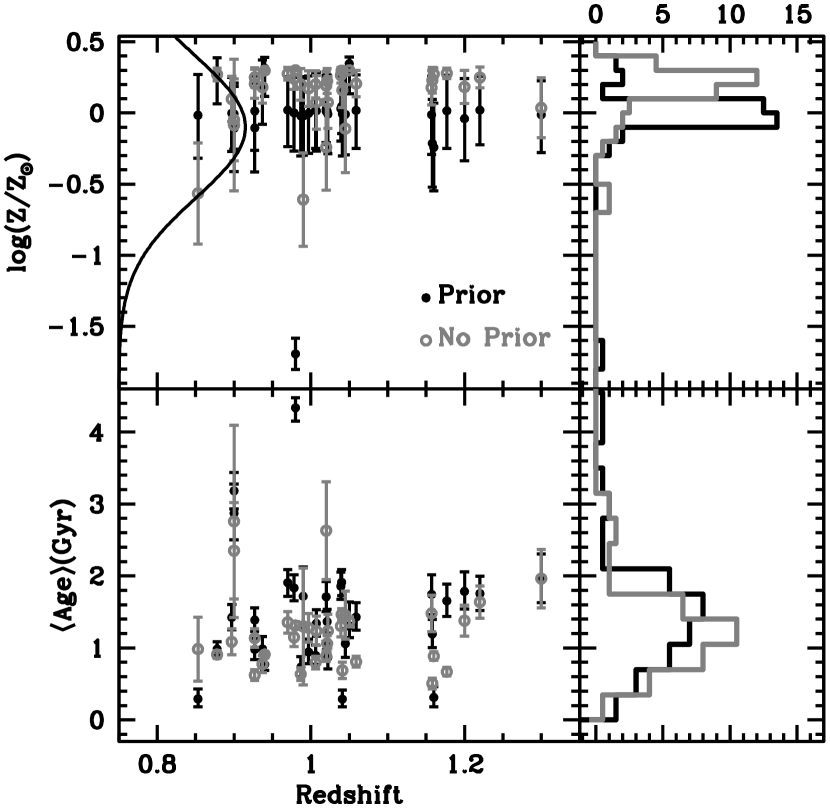
Figure 17.— Comparison of bulge age distribution and bulge metallicity for EXP models with and without a metallicity prior. The age histogram does not show any appreciable change. The metallicity histogram without a prior (grey) peak at slightly higher metallicities – as illustrated in Figure 15 – compared to the metallicity histogram (black) with prior, but it is nevertheless compatible given the typical uncertainty (of order 0.3 dex) in estimates of metallicity from unresolved stellar populations.

Appendix B Effect of Disk Contamination on Bulge Ages

In order to assess the effect of disk contamination on the age and metallicity estimates, we performed an extraction of the SED of the disk component for a small sub-sample of galaxies. This corresponds to the stacking of two strips (5 pixels wide) at an approximate distance of 10 pixels on either side of the center of the galaxy. When comparing the observed spectra with synthetic models, we assume that a fraction of the flux in each galaxy comes from the disk. Hence, for each choice of parameters, a synthetic SED is obtained, and a fraction $f_{D}$ of the disk SED is added to this spectrum, before performing a maximum likelihood analysis. This fraction is measured in the $i^{\prime}$-band (F775W). Figure 18 shows the resulting ages and metallicities for four galaxies from our sample as a function of disk contamination. The 95% confidence levels are shown as error bars. The ages and metallicities are shown in the same plot, as solid and open dots, respectively. One can see that the effect of disk contamination is small, as expected from the weak color gradients found in the images. This result is consistent with the idea that the inner disk of galaxies is as old as the bulge (e.g., Peletier & Balcells, 1996).

Figure 18.— Effect of disk contamination on the predictions of age and metallicity. The solid (empty) dots show the estimated average age (metallicity) for a grid of exponentially-decaying star-formation histories. The 95% confidence levels are shown as error bars. The result is presented as a function of the contamination of the disk, as measured in the F775W band (see text for details).

Table 1Our Sample - HUDF IDs, Coordinates, Optical Magnitudes and Colors

HUDF	RA (J2000)	DEC (J2000)	$B$	$V$	$i^{\prime}$	$z^{\prime}$	($V$–$z^{\prime}$)†
ID	(deg)	(deg)	(mag)	(mag)	(mag)	(mag)	color
501	53.1677662	$-$27.8166951	24.73	24.47	23.94	23.40	1.068
521	53.1699372	$-$27.8178736	26.27	25.98	25.28	24.94	1.041
901	53.1681788	$-$27.8129432	24.44	24.03	23.35	23.06	0.970
3048	53.1659121	$-$27.7997159	26.63	26.21	25.40	25.17	1.041
3299	53.1923333	$-$27.7978741	25.71	25.40	25.00	24.59	0.817
3372	53.1761793	$-$27.7961337	22.90	22.34	21.64	21.25	1.095
3373	53.1668679	$-$27.7976989	24.48	24.43	23.94	23.77	0.662
3613	53.1567527	$-$27.7955981	23.80	23.34	22.63	22.12	1.219
4072	53.1278092	$-$27.7950828	24.66	24.49	24.26	23.73	0.759
4084	53.1278372	$-$27.7947976	24.61	24.44	24.05	23.56	0.888
4438	53.1376781	$-$27.7919373	23.58	23.13	22.44	22.08	1.049
4491	53.1675702	$-$27.7925214	23.93	23.68	23.24	22.89	0.791
4591	53.1713278	$-$27.7929428	25.08	24.83	24.16	23.84	0.990
5190	53.1450905	$-$27.7894219	24.22	24.00	23.70	23.17	0.827
5405	53.1606000	$-$27.7897302	26.09	25.79	25.12	24.64	1.150
5417	53.1661791	$-$27.7875215	23.10	22.61	21.97	21.48	1.135
5658	53.1740361	$-$27.7880062	24.99	24.61	23.99	23.43	1.178
5805	53.1920649	$-$27.7871824	23.91	23.58	23.04	22.57	1.011
5989	53.1609549	$-$27.7864996	24.81	24.58	24.05	23.55	1.028
6079	53.1394080	$-$27.7867760	25.76	25.35	24.78	24.12	1.222
6785	53.1915603	$-$27.7826687	24.15	23.88	23.57	22.97	0.907
6821	53.1782201	$-$27.7830771	24.13	23.90	23.47	23.04	0.865
7036	53.1903447	$-$27.7820005	24.43	24.29	24.09	23.57	0.714
7112	53.1658806	$-$27.7815379	24.65	24.09	23.41	22.83	1.258
7559	53.1587381	$-$27.7705348	23.93	23.54	22.86	22.48	1.057
8125	53.1729989	$-$27.7778393	23.95	23.85	23.45	23.14	0.716
8551	53.1517635	$-$27.7754183	23.90	23.42	22.71	22.25	1.173
8585	53.1479310	$-$27.7739569	22.42	22.13	21.63	21.15	0.973
9018	53.1470806	$-$27.7784243	24.44	24.32	23.96	23.66	0.663
9125	53.1663274	$-$27.7685923	24.13	23.83	23.36	22.71	1.121
9183	53.1601763	$-$27.7693039	24.86	24.80	24.40	24.18	0.611
9341	53.1598624	$-$27.7668404	24.88	24.68	24.12	23.72	0.953
9444	53.1554162	$-$27.7660748	25.81	24.91	24.04	23.34	1.572
9759	53.1596949	$-$27.7622834	24.76	24.62	24.34	23.82	0.803

Note. — Magnitudes are in the AB photometric system.

Table 2Our Sample - IDs, Coordinates and Redshifts

HUDF	RA (J2000)	DEC (J2000)	$z^{a}$	$z^{b}$	$z^{c}$
(ID)	(deg)	(deg)	phot	VLT	SED Fit
501	53.1677662	$-$27.8166951	1.07	$\cdots$	1.02
521	53.1699372	$-$27.8178736	1.04	$\cdots$	0.99
901	53.1681788	$-$27.8129432	0.94	$\cdots$	0.88
3048	53.1659121	$-$27.7997159	0.84	$\cdots$	0.85
3299	53.1923333	$-$27.7978741	1.06	1.221	1.20
3372	53.1761793	$-$27.7961337	1.04	0.996	0.98
3373	53.1668679	$-$27.7976989	0.89	$\cdots$	0.93
3613	53.1567527	$-$27.7955981	1.07	1.097	0.98
4072	53.1278092	$-$27.7950828	1.27	1.189d	1.20
4084	53.1278372	$-$27.7947976	1.08	$\cdots$	1.06
4438	53.1376781	$-$27.7919373	1.04	0.998	0.97
4491	53.1675702	$-$27.7925214	1.05	$\cdots$	1.01
4591	53.1713278	$-$27.7929428	0.92	$\cdots$	0.90
5190	53.1450905	$-$27.7894219	1.22	1.316	1.18
5405	53.1606000	$-$27.7897302	1.07	1.096	0.90
5417	53.1661791	$-$27.7875215	1.10	1.097	1.03
5658	53.1740361	$-$27.7880062	1.07	1.096	1.05
5805	53.1920649	$-$27.7871824	1.05	$\cdots$	1.02
5989	53.1609549	$-$27.7864996	0.95	1.135	1.00
6079	53.1394080	$-$27.7867760	1.16	1.298	1.16
6785	53.1915603	$-$27.7826687	1.14	$\cdots$	1.29
6821	53.1782201	$-$27.7830771	1.07	$\cdots$	1.02
7036	53.1903447	$-$27.7820005	1.21	0.743d	1.16
7112	53.1658806	$-$27.7815379	1.07	$\cdots$	1.04
7559	53.1587381	$-$27.7705348	0.96	$\cdots$	0.93
8125	53.1729989	$-$27.7778393	1.05	$\cdots$	1.04
8551	53.1517635	$-$27.7754183	1.05c	1.047	1.05
8585	53.1479310	$-$27.7739569	0.97	1.088	1.05
9018	53.1470806	$-$27.7784243	0.95	$\cdots$	0.99
9125	53.1663274	$-$27.7685923	1.20	1.295	1.21
9183	53.1601763	$-$27.7693039	0.94	$\cdots$	0.94
9341	53.1598624	$-$27.7668404	1.03	$\cdots$	1.01
9444	53.1554162	$-$27.7660748	1.07	1.096	1.02
9759	53.1596949	$-$27.7622834	1.34	$\cdots$	1.22

References

- Abraham et al. (1999) Abraham, R. G., Ellis, R. S., Fabian, A. C., Tanvir, N. R., & Glazebrook, K. 1999, MNRAS, 303, 641
- Athanassoula (2005) Athanassoula, E. 2005, MNRAS, 358, 1477
- Athanassoula (2008) Athanassoula, E. 2008, IAU Symposium 245 “Galactic bulges”, M. Bureau et al. eds (arXiv:0802.0151)
- Balogh et al. (1999) Balogh, M.L., et al. 1999, ApJ, 527, 54
- Balogh et al. (2004) Balogh, M.L., Baldry, I. K., Nichol, R., Miller, C., Bower, R., & Glazebrook, K. 2004, ApJ, 615, L101
- Baugh et al. (1996) Baugh, C. M., Cole, S., & Frenk, C. S. 1996, MNRAS, 283, 1361
- Beckwith et al. (2006) Beckwith, S., et al. 2006, AJ, 132, 1729
- Bershady et al. (2000) Bershady, M. A., Jangren, A., & Conselice, C. J. 2000, AJ, 119, 2645
- Bouwens et al. (1999) Bouwens, R., Cayón, L., & Silk, J. 1999, ApJ, 516, 77
- Bruzual & Charlot (2003) Bruzual, G., & Charlot, S. 2003, MNRAS, 344, 1000
- Carollo et al. (2007) Carollo, C. M., Scarlata, C., Stiavelli, M., Wyse, R. F. G., & Mayer, L. 2007, ApJ, 658, 960
- Chabrier (2003) Chabrier, G. 2003, PASP, 115, 763
- Coe et al. (2006) Coe, D., Benítez, N., Sánchez, S. F., Jee, M., Bouwens, R., & Ford, H. 2006, AJ, 132, 926
- Conselice et al. (2000) Conselice, C. J., Bershady, M. A., & Jangren, A. 2000, ApJ, 529, 886
- Conselice (2003) Conselice, C. J. 2003, ApJS, 147, 1
- Conselice et al. (2005) Conselice, C. J., Blackburne, J. A., & Papovich, C. 2005, ApJ, 620, 564
- Courteau et al. (1996) Courteau, S., de Jong, R. S., & Broeils, A. H. 1996, ApJ, 457, L73
- de Jong (1996) de Jong, R. S. 1996, A&AS, 118, 557
- Dong & De Robertis (2006) Dong, X. Y. & De Robertis, M. M. 2006, AJ, 131, 1236
- Driver et al. (2006) Driver, S. P., et al. 2006, MNRAS, 368, 414
- Drory & Fisher (2007) Drory, N. & Fisher, D. B. 2007, ApJ, 664, 640
- Ellis et al. (2001) Ellis, R. S., Abraham, R. G., & Dickinson, M. 2001, ApJ, 551, 111
- Elmegreen et al. (2005) Elmegreen, D. M., Elmegreen, B. G., Rubin, D. S., & Schaffer, M. A. 2005, ApJ, 631, 85
- Ferreras & Silk (2000) Ferreras, I., & Silk, J. 2000, MNRAS, 316, 786
- Ferreras et al. (2005) Ferreras, I., Lisker, T., Carollo, C. M., Lilly, S. J., & Mobasher, B. 2005, ApJ, 635, 243
- Grazian et al. (2006) Grazian, A., et al. 2006, A&A, 449, 951
- Hathi et al. (2008a) Hathi, N. P., Malhotra, S., & Rhoads, J. 2008a, ApJ, 673, 686
- Hathi et al. (2008b) Hathi, N. P., Jansen, R. A., Windhorst, R. A., Cohen, S. H., Keel, W. C., Corbin, M. R., & Ryan, R. E., Jr. 2008b, AJ, 135, 156
- Hernquist & Mihos (1995) Hernquist, L. & Mihos, J. C. 1995, ApJ, 448, 41
- Kauffmann et al. (1993) Kauffmann, G., White, S. D. M., & Guiderdoni, B. 1993, MNRAS, 264, 201
- Kauffmann et al. (2003) Kauffmann, G., et al. 2003, MNRAS, 341, 33
- Koekemoer et al. (2002) Koekemoer, A. M., Fruchter, A. S., Hook, R. N., & Hack, W. 2002, The 2002 HST Calibration Workshop, ed. S. Arribas, A. Koekemoer, and B. Whitmore (Baltimore:STScI), 337
- Koo et al. (2005) Koo, D. C., et al. 2005, ApJS, 157, 175
- Kormendy & Kennicutt (2004) Kormendy, J. & Kennicutt, R. C. 2004, ARA&A, 42, 603
- Le Fèvre et al. (2005) Le Fèvre, O., et al. 2005, A&A, 439, 845
- Liu et al. (2008) Liu, X., Shapley, A., Coil, A., Brinchmann, J., & Ma, C-P. 2008, ApJ, 678, 758
- MacArthur et al. (2004) MacArthur, L. A., Courteau, S., Bell, E., & Holtzman, J. A. 2004, ApJS, 152, 175
- MacArthur et al. (2008) MacArthur, L. A., Ellis, R. S., Treu, T., Vivian, V., Bundy, K., Moran, S. M. 2008, ApJ, 680, 70
- Malhotra et al. (2005) Malhotra, S., Rhoads, J. E., Pirzkal, N., et al. 2005, ApJ, 626, 666
- Menanteau et al. (2001) Menanteau, F., Abraham, R. G., & Ellis, R. S. 2001, MNRAS, 322, 1
- Oke & Gunn (1983) Oke, J. B., & Gunn, J.E. 1983, ApJ, 266, 713
- Padmanabhan et al. (2004) Padmanabhan, N., et al. 2004, New Astronomy, 9, 329
- Pasquali et al. (2006a) Pasquali, A., Pirzkal, N., Larsen, S., Walsh, J. R., & Kümmel, M. 2006a, PASP, 118, 270
- Pasquali et al. (2006b) Pasquali, A., et al. 2006b, ApJ, 636, 115
- Peletier & Balcells (1996) Peletier, R. F. & Balcells, M. 1996, AJ, 111, 2238
- Peng et al. (2002) Peng, C. Y., Ho, L. C., Impey, C. D., & Rix, H-W. 2002, AJ, 124, 266
- Pirzkal et al. (2004) Pirzkal, N., et al. 2004, ApJS, 154, 501
- Pirzkal et al. (2005) Pirzkal, N., et al. 2005, ApJ, 622, 319
- Ryan et al. (2007) Ryan, R. E., Jr., Hathi, N. P., Cohen, S. H., et al. 2007, ApJ, 668, 839
- Saha (2003) Saha, P. 2003, Principles of Data Analysis, Cappella Archive.
- Salpeter (1955) Salpeter, E. E. 1955, ApJ, 121, 161
- Schiavon et al. (2006) Schiavon, R., et al. 2006, ApJ, 651, L93
- Sérsic (1968) Sérsic, J. L. 1968, Atlas de galaxias australes
- Shapley et al. (2005) Shapley, A. E., Coil, A., Ma, C-P., & Bundy, K. 2005, ApJ, 635, 1006
- Sheth et al. (2005) Sheth, K., Vogel, S. N., Regan, M. W., Thornley, M. D., & Teuben, P. J. 2005, ApJ, 632, 217
- Sheth et al. (2008) Sheth, K., et al. 2008, ApJ, 675, 1141
- Simien & de Vaucouleurs (1986) Simien, F., & de Vaucouleurs, G. 1986, ApJ, 302, 564
- Thielemann et al. (1996) Thielemann, F-K., Nomoto, K., & Hashimoto, M. 1996, ApJ, 460, 408
- Thomas & Davies (2006) Thomas, D., & Davies, R. L. 2006, MNRAS, 366, 510
- van den Bosch (1998) van den Bosch, F. C. 1998, ApJ, 507, 601
- van den Hoek & Groenewegen (1997) van den Hoek, L. B., & Groenewegen, M. A. T. 1997, A&AS, 123, 305
- Vanzella et al. (2006) Vanzella, E., Cristiani, S., Dickinson, M., et al. 2006, A&A, 454, 423
- Vanzella et al. (2008) Vanzella, E., et al. 2008, A&A, 478, 83
- Williams et al. (1996) Williams, R. E., et al. 1996, AJ, 112, 1335
- Windhorst et al. (2002) Windhorst, R. A., et al. 2002, ApJS, 143, 113