Splitting Polytopes

Abstract.

A split of a polytope $P$ is a (regular) subdivision with exactly two maximal cells. It turns out that each weight function on the vertices of $P$ admits a unique decomposition as a linear combination of weight functions corresponding to the splits of $P$ (with a split prime remainder). This generalizes a result of Bandelt and Dress [Adv. Math. 92 (1992)] on the decomposition of finite metric spaces.

Introducing the concept of compatibility of splits gives rise to a finite simplicial complex associated with any polytope $P$, the split complex of $P$. Complete descriptions of the split complexes of all hypersimplices are obtained. Moreover, it is shown that these complexes arise as subcomplexes of the tropical (pre-)Grassmannians of Speyer and Sturmfels [Adv. Geom. 4 (2004)].

1. Introduction

A real-valued weight function $w$ on the vertices of a polytope $P$ in ${\mathbb{R}}^{d}$ defines a polytopal subdivision of $P$ by way of lifting to ${\mathbb{R}}^{d+1}$ and projecting the lower hull back to ${\mathbb{R}}^{d}$. The set of all weight functions on $P$ has the natural structure of a polyhedral fan, the secondary fan ${\rm SecFan}(P)$. The rays of ${\rm SecFan}(P)$ correspond to the coarsest (regular) subdivisions of $P$. This paper deals with the coarsest subdivisions with precisely two maximal cells. These are called splits.

Hirai proved in [17] that an arbitrary weight function on $P$ admits a canonical decomposition as a linear combination of split weights with a split prime remainder. This generalizes a classical result of Bandelt and Dress [2] on the decomposition of finite metric spaces, which proved to be useful for applications in phylogenomics; e.g., see Huson and Bryant [19]. We give a new proof of Hirai’s split decomposition theorem which establishes the connection to the theory of secondary fans developed by Gel^′fand, Kapranov, and Zelevinsky [14].

Our main contribution is the introduction and the study of the split complex of a polytope $P$. This comes about as the clique complex of the graph defined by a compatibility relation on the set of splits of $P$. A first example is the boundary complex of the polar dual of the $(n-3)$-dimensional associahedron, which is isomorphic to the split complex of an $n$-gon. A focus of our investigation is on the hypersimplices ${\Delta(k,n)}$, which are the convex hulls of the $0/1$-vectors of length $n$ with exactly $k$ ones. We classify all splits of the hypersimplices together with their compatibility relation. This describes the split complexes of the hypersimplices.

Tropical geometry is concerned with the tropicalization of algebraic varieties. An important class of examples is formed by the tropical Grassmannians ${{\mathscr{G}}_{k,n}}$ of Speyer and Sturmfels [38], which are the tropicalizations of the ordinary Grassmannians of $k$-dimensional subspaces of an $n$-dimensional vector space (over some field). It is a challenge to obtain a complete description of ${{\mathscr{G}}_{k,n}}$ even for most fixed values of $k$ and $n$. A better behaved close relative of ${{\mathscr{G}}_{k,n}}$ is the tropical pre-Grassmannian ${{\rm pre-}{\mathscr{G}}_{k,n}}$ arising from tropicalizing the ideal of quadratic Plücker relations. This is a subfan of the secondary fan of ${\Delta(k,n)}$, and its rays correspond to coarsest subdivisions of ${\Delta(k,n)}$ whose (maximal) cells are matroid polytopes; see Kapranov [24] and Speyer [36]. As one of our main results we prove that the split complex of ${\Delta(k,n)}$ is a subcomplex of ${{\rm pre-}{\mathscr{G}}^{\prime}_{k,n}}$, the intersection of the fan ${{\rm pre-}{\mathscr{G}}_{k,n}}$ with the unit sphere in ${\mathbb{R}}^{\tbinom{n}{k}}$. Moreover, we believe that our approach can be extended further to obtain a deeper understanding of the tropical (pre-)Grassmannians. To follow this line, however, is beyond the scope of this paper.

The paper is organized as follows. We start out with the investigation of general weight functions on a polytope $P$ and their coherence. Two weight functions are coherent if there is a common refinement of the subdivisions that they induce on $P$. As an essential technical device for the subsequent sections we introduce the coherency index of two weight functions on $P$. This generalizes the definition of Koolen and Moulton for ${\Delta(2,n)}$ [28], Section 4.1.

The third section then deals with splits of polytopes and the corresponding weight functions. As a first result we give a concise new proof of the split decomposition theorems of Bandelt and Dress [2], Theorem 3, and Hirai [17], Theorem 2.2.

A split subdivision of the polytope $P$ is clearly determined by the affine hyperplane spanned by the unique interior cell of codimension $1$. A set of splits is compatible if any two of the corresponding split hyperplanes do not meet in the (relative) interior of $P$. The split complex ${\rm Split}(P)$ is the abstract simplicial complex of compatible sets of splits of $P$. It is an interesting fact that the subdivision of $P$ induced by a sum of weights corresponding to a compatible system of splits is dual to a tree. In this sense ${\rm Split}(P)$ can always be seen as a “space of trees”.

In Section 5 we study the hypersimplices ${\Delta(k,n)}$. Their splits are classified and explicitly enumerated. Moreover, we characterize the compatible pairs of splits. The purpose of the short Section 6 is to specialize our results for arbitrary hypersimplices to the case $k=2$. A metric on a finite set of $n$ points yields a weight function on ${\Delta(2,n)}$, and hence all the previous results can be interpreted for finite metric spaces. This is the classical situation studied by Bandelt and Dress [1, 2]. Notice that some of their results had already been obtained by Isbell much earlier [20].

Section 7 bridges the gap between the split theory of the hypersimplices and matroid theory. This way, as one key result, we can prove that the split complex of the hypersimplex ${\Delta(k,n)}$ is a subcomplex of the tropical pre-Grassmannian ${{\rm pre-}{\mathscr{G}}^{\prime}_{k,n}}$. We conclude the paper with a list of open questions.

2. Coherency of Weight Functions

Let $P\subset{\mathbb{R}}^{d+1}$ be a polytope with vertices $v_{1},\dots,v_{n}$. We form the $n\times(d+1)$-matrix $V$ whose rows are the vertices of $P$. For technical reasons we make the assumption that $P$ is $d$-dimensional and that the (column) vector $\mathbbm{1}:=(1,\dots,1)$ is contained in the linear span of the columns of $V$. In particular, this implies that $P$ is contained in some affine hyperplane which does not contain the origin. A weight function $w:\operatorname{Vert}{P}\to{\mathbb{R}}$ of $P$ can be written as a vector in ${\mathbb{R}}^{n}$. Now each weight function $w$ of $P$ gives rise to the unbounded polyhedron

$${{\mathscr{E}}_{w}(P)}\ :=\ \left\{x\in{\mathbb{R}}^{d+1}\vphantom{Vx\geq-w}\,\right.\left|\,\vphantom{x\in{\mathbb{R}}^{d+1}}Vx\geq-w\right\}\,,$$

the envelope of $P$ with respect to $w$. We refer to Ziegler [45] for details on polytopes.

If $w_{1}$ and $w_{2}$ are both weight functions of $P$, then $Vx\geq-w_{1}$ and $Vy\geq-w_{2}$ implies $V(x+y)\geq-(w_{1}+w_{2})$. This yields the inclusion

(1) $${{\mathscr{E}}_{w_{1}}(P)}+{{\mathscr{E}}_{w_{2}}(P)}\ \subseteq\ {{\mathscr{E}}_{w_{1}+w_{2}}(P)}\,.$$

If equality holds in (1) then $(w_{1},w_{2})$ is called a coherent decomposition of $w=w_{1}+w_{2}$. (Note that this must not be confused with the notion of “coherent subdivision” which is sometimes used instead of “regular subdivision”.)

Example 1.

We consider a hexagon $H\subset{\mathbb{R}}^{3}$ whose vertices are the columns of the matrix

$${V}^{\sf T}\ =\ \begin{pmatrix}1&1&1&1&1&1\\ 0&1&2&2&1&0\\ 0&0&1&2&2&1\end{pmatrix}$$

and three weight functions $w_{1}=(0,0,1,1,0,0)$, $w_{2}=(0,0,0,1,1,0)$, and $w_{3}=(0,0,2,3,2,0)$. Again we identify a matrix with the set of its rows. A direct computation then yields that $w_{1}+w_{2}$ is not coherent, but both $w_{1}+w_{3}$ and $w_{2}+w_{3}$ are coherent.

Each face of a polyhedron, that is, the intersection with a supporting hyperplane, is again a polyhedron, and it can be bounded or not. A polyhedron is pointed if it does not contain an affine subspace or, equivalently, its lineality space is trivial. This implies that the set of all bounded faces is non-empty and forms a polytopal complex. This polytopal complex is always contractible (see Hirai [16, Lemma 4.5]). The polytopal complex of bounded faces of the polyhedron ${{\mathscr{E}}_{w}(P)}$ is called the tight span of $P$ with respect to $w$, and it is denoted by ${{\mathscr{T}}_{w}(P)}$.

Lemma 2.

Let $w=w_{1}+w_{2}$ be a decomposition of weight functions of $P$. Then the following statements are equivalent.

1. The decomposition $(w_{1},w_{2})$ is coherent,

2. ${{\mathscr{T}}_{w}(P)}\subseteq{{\mathscr{T}}_{w_{1}}(P)}+{{\mathscr{T}}_{w_{2}}(P)}$ ,

3. ${{\mathscr{T}}_{w}(P)}\subseteq{{\mathscr{E}}_{w_{1}}(P)}+{{\mathscr{E}}_{w_{2}}(P)}$ ,

4. each vertex of ${{\mathscr{T}}_{w}(P)}$ can be written as a sum of a vertex of ${{\mathscr{T}}_{w_{1}}(P)}$ and a vertex of ${{\mathscr{T}}_{w_{2}}(P)}$.

For a similar statement in the special case where $P$ is a second hypersimplex (see Section 5 below) see Koolen and Moulton [27], Lemma 1.2.

Proof.

If $(w_{1},w_{2})$ is coherent then by definition ${{\mathscr{E}}_{w}(P)}={{\mathscr{E}}_{w_{1}}(P)}+{{\mathscr{E}}_{w_{2}}(P)}$. Each face $F$ of the Minkowski sum of two polyhedra is the Minkowski sum of two faces $F_{1},F_{2}$, one from each summand. Now $F$ is bounded if and only if $F_{1}$ and $F_{2}$ are bounded. This proves that (i) implies (ii).

Clearly, (ii) implies (iii). Moreover, (iii) implies (iv) by the same argument on Minkowski sums as above.

To complete the proof we have to show that (i) follows from (iv). So assume that each vertex of ${{\mathscr{T}}_{w}(P)}$ can be written as a sum of a vertex of ${{\mathscr{T}}_{w_{1}}(P)}$ and a vertex of ${{\mathscr{T}}_{w_{2}}(P)}$, and let $x\in{{\mathscr{E}}_{w}(P)}$. Then $x$ can be written as $x=y+r$ where $y\in{{\mathscr{T}}_{w}(P)}$ and r is a ray of ${{\mathscr{E}}_{w}(P)}$, that is, $z+\lambda r\in{{\mathscr{E}}_{w}(P)}$ for all $z\in{{\mathscr{E}}_{w}(P)}$ and all $\lambda\geq 0$. It follows that $Vr\leq 0$. By assumption there are vertices $y_{1}$ and $y_{2}$ of ${{\mathscr{T}}_{w_{1}}(P)}$ and ${{\mathscr{T}}_{w_{2}}(P)}$ such that $y=y_{1}+y_{2}$. Setting $x_{1}:=y_{1}+r$ and $x_{2}:=y_{2}$ we have $x=x_{1}+x_{2}$ with $x_{2}\in{{\mathscr{E}}_{w_{2}}(P)}$. Computing

$$Vx_{1}\ =\ V(y_{1}+r)\ \leq\ Vy_{1}+Vr\ \leq\ -w_{1}+0\ =\ -w_{1}\,,$$

we infer that $x_{1}\in{{\mathscr{E}}_{w_{1}}(P)}$, and hence $w_{1}$ and $w_{2}$ are coherent. ∎

We recall basic facts about cone polarity. For an arbitrary pointed polyhedron $X\subset{\mathbb{R}}^{d+1}$ there exists a unique polyhedral cone $C(X)\subset{\mathbb{R}}^{d+2}$ such that $X=\left\{x\in{\mathbb{R}}^{d+1}\vphantom{(1,x)\in C(P)}\,\right.\left|\,\vphantom{x\in{\mathbb{R}}^{d+1}}(1,x)\in C(P)\right\}$. If $X$ is given in inequality description $X=\left\{x\in{\mathbb{R}}^{d+1}\vphantom{Ax\geq b}\,\right.\left|\,\vphantom{x\in{\mathbb{R}}^{d+1}}Ax\geq b\right\}$ one has

$$C(X)\ =\ \left\{y\in{\mathbb{R}}^{d+2}\vphantom{\begin{pmatrix}1&0\\ -b&A\end{pmatrix}y\geq 0}\,\right.\left|\,\vphantom{y\in{\mathbb{R}}^{d+2}}\begin{pmatrix}1&0\\ -b&A\end{pmatrix}y\geq 0\right\}\,.$$

If $X$ is given in a vertex-ray description $P=\operatorname{conv}V+\operatorname{pos}R$ one has

$$C(X)\ =\ \operatorname{pos}\begin{pmatrix}\mathbbm{1}&V\\ 0&R\end{pmatrix}\,.$$

For any set $M\subseteq{\mathbb{R}}^{d+2}$ its cone polar is defined as $M^{\circ}:=\{y\in{\mathbb{R}}^{d+2}\,|\,\langle{x},{y}\rangle\geq 0\text{ for all $x\in M$}\}$. If $C=\operatorname{pos}A$ is a cone it is easily seen that $C^{\circ}=\{y\in{\mathbb{R}}^{d+2}\,|\,Ay\geq 0\}$ and that ${(C^{\circ})}^{\circ}=C$. The cone $C^{\circ}$ is called the polar dual cone of $C$. Two polyhedra $X$ and $Y$ are polar duals if the corresponding cones $C(X)$ and $C(Y)$ are. The face lattices of dual cones are anti-isomorphic.

For the following our technical assumptions from the beginning come into play. Again let $P$ be a $d$-polytope in ${\mathbb{R}}^{d+1}$ such that $\mathbbm{1}$ is contained in the column span of the matrix $V$ whose rows are the vertices of $P$. The standard basis vectors of ${\mathbb{R}}^{d+1}$ are denoted by $e_{1},\dots,e_{d+1}$.

Proposition 3.

The polyhedron ${{\mathscr{E}}_{w}(P)}$ is affinely equivalent to the polar dual of the polyhedron

$${{\mathscr{L}}_{w}(P)}\ :=\operatorname{conv}\left\{v+w(v)e_{d+1}\vphantom{v\in\operatorname{Vert}{P}}\,\right.\left|\,\vphantom{v+w(v)e_{d+1}}v\in\operatorname{Vert}{P}\right\}\,+\,{{\mathbb{R}}_{\geq 0}}e_{d+1}\,.$$

Moreover, the face poset of ${{\mathscr{T}}_{w}(P)}$ is anti-isomorphic to the face poset of the interior lower faces (with respect to the last coordinate) of ${{\mathscr{L}}_{w}(P)}$.

Proof.

Note first, that by our assumption that $\mathbbm{1}$ is in the column span of $V$, up to a linear transformation of ${\mathbb{R}}^{d+1}$, we can assume that $V=(\bar{V},\mathbbm{1})$ for an $n\times d$-matrix $\bar{V}$. This yields

$$C({{\mathscr{E}}_{w}(P)})\ =\ \left\{x\in{\mathbb{R}}^{d+2}\vphantom{\begin{pmatrix}1&0&0\\ w&\bar{V}&\mathbbm{1}\end{pmatrix}x\geq 0}\,\right.\left|\,\vphantom{x\in{\mathbb{R}}^{d+2}}\begin{pmatrix}1&0&0\\ w&\bar{V}&\mathbbm{1}\end{pmatrix}x\geq 0\right\}.$$

On the other hand we have

$$C({{\mathscr{L}}_{w}(P)})\ =\ \operatorname{pos}\begin{pmatrix}\mathbbm{1}&\bar{V}&w\\ 0&0&1\end{pmatrix},$$

which is linearly isomorphic to $\bar{C}=\operatorname{pos}\left(\begin{smallmatrix}w&\mathbbm{1}&\bar{V}\\ 1&0&0\end{smallmatrix}\right)$ by a coordinate change, so ${{\mathscr{E}}_{w}(P)}$ and ${{\mathscr{L}}_{w}(P)}$ are polar duals, up to linear transformations.

This way we have obtained an anti-isomorphism of the face lattices of $C({{\mathscr{E}}_{w}(P)})$ and $C({{\mathscr{L}}_{w}(P)})$. A face $F$ of ${{\mathscr{E}}_{w}(P)}$ is bounded if and only if no generator of $C({{\mathscr{E}}_{w}(P)})$ with first coordinate equal to zero is smaller then $F$ in the face lattice. In the dual view, this means that the corresponding face $F^{\prime}$ of ${{\mathscr{L}}_{w}(P)}$ is greater then a facet which is parallel to the last coordinate axis in the face lattice of $C({{\mathscr{L}}_{w}(P)})$. But this exactly means that $F^{\prime}$ is a lower face. So the lattice anti-isomorphism of $C({{\mathscr{E}}_{w}(P)})$ and $C({{\mathscr{L}}_{w}(P)})$ induces a poset anti-isomorphism between ${{\mathscr{T}}_{w}(P)}$ and the interior lower faces of ${{\mathscr{L}}_{w}(P)}$. ∎

The lower faces of ${{\mathscr{L}}_{w}(P)}$ (with respect to the last coordinate) are precisely its bounded faces. By projecting back to $\operatorname{aff}{P}$ in the $e_{d+1}$-direction, the polytopal complex of bounded faces of ${{\mathscr{L}}_{w}(P)}$ induces a polytopal decomposition ${\Sigma_{w}(P)}$ of $P$. Note that we only allow the vertices of $P$ as vertices of any subdivision of $P$. A polytopal subdivision which arises in this way is called regular. Two weight functions are equivalent if they induce the same subdivision. This allows for one more characterization extending Lemma 2.

Corollary 4.

A decomposition $w=w_{1}+w_{2}$ of weight functions of $P$ is coherent if and only if the subdivision ${\Sigma_{w}(P)}$ is the common refinement of the subdivisions ${\Sigma_{w_{1}}(P)}$ and ${\Sigma_{w_{2}}(P)}$.

Proof.

By Lemma 2, the decomposition $w_{1}+w_{2}$ is coherent if and only if each vertex $x$ of ${{\mathscr{T}}_{w}(P)}$ is the sum of a vertex $x_{1}$ of ${{\mathscr{T}}_{w_{1}}(P)}$ and a vertex $x_{2}$ of ${{\mathscr{T}}_{w_{2}}(P)}$. In terms of the duality proved in Proposition 3 the vertex $x$ corresponds to the maximal cell $F_{w}(x):=\operatorname{conv}\{v\in\operatorname{Vert}P\,|\,\langle{v},{x}\rangle=-w\}$ of ${\Sigma_{w}(P)}$. Similarly, $x_{1}$ and $x_{2}$ corresponds to the cells $F_{w_{1}}(x_{1})$ and $F_{w_{2}}(x_{2})$ of ${\Sigma_{w_{1}}(P)}$ and ${\Sigma_{w_{2}}(P)}$, respectively. In fact, we have $F_{w}(x)=F_{w_{1}}(x_{1})\cap F_{w_{2}}(x_{2})$, and so ${\Sigma_{w}(P)}$ is the common refinement of ${\Sigma_{w_{1}}(P)}$ and ${\Sigma_{w_{2}}(P)}$. The converse follows similarly. ∎

Example 5.

In Example 1 the tight spans of the three weight functions of the hexagon are line segments:

$${{\mathscr{T}}_{w_{1}}(H)}\ =\ [0,(1,-1,0)]\,,\quad{{\mathscr{T}}_{w_{2}}(H)}\ =\ [0,(1,0,-1)]\,,\quad\text{and}\quad{{\mathscr{T}}_{w_{3}}(H)}\ =\ [0,(1,-1,-1)]\,.$$

Remark 6.

Interesting special cases of tight spans include the following. Finite metric spaces (on $n$ points) give rise to weight functions on the second hypersimplex $P={\Delta(2,n)}$. In this case the tight span can be interpreted as a “space” of trees which are candidates to fit the given metric. This has been studied by Bandelt and Dress [2], and this is the context in which the name “tight span” was used first. See also Section 6 below.

If $P$ is a product of two simplices, the tight span of a lifting function gives rise to a tropical polytope introduced by Develin and Sturmfels [9], the cells in the resulting regular decomposition of $P$ are the polytropes of [23].

If $P$ spans the affine hyperplane $x_{1}=1$ and if we consider the weight function defined by $w(v)=v_{2}^{2}+v_{3}^{2}+\dots+v_{d+1}^{2}$ for each vertex $v$ of $P$ then the tight span ${{\mathscr{T}}_{w}(P)}$ is isomorphic to the subcomplex of bounded faces of the Voronoi diagram of $\operatorname{Vert}{P}$. All maximal cells of the Voronoi diagram are unbounded and hence the tight span is at most $(d-1)$-dimensional. The subdivision ${\Sigma_{w}(P)}$ is then isomorphic to the Delone decomposition of $\operatorname{Vert}{P}$.

Let $w$ and $w^{\prime}$ be weight functions of our polytope $P$. We want to have a measure which expresses to what extent the pair of weight functions $(w^{\prime},w-w^{\prime})$ deviates from coherence (if at all). The coherency index of $w$ with respect to $w^{\prime}$ is defined as

(2) $$\alpha^{w}_{w^{\prime}}\ :=\ \min_{x\in\operatorname{Vert}{{{\mathscr{E}}_{w}(P)}}}\left\{\max_{x^{\prime}\in\operatorname{Vert}{{{\mathscr{E}}_{w^{\prime}}(P)}}}\left\{\min_{v\in V_{w^{\prime}}(x^{\prime})}\left\{\frac{\langle{v},{x}\rangle+w(v)}{\langle{v},{x^{\prime}}\rangle+w^{\prime}(v)}\right\}\right\}\right\}\,,$$

where $V_{w^{\prime}}(x^{\prime})=\left\{v\in\operatorname{Vert}{P}\vphantom{\langle{v},{x^{\prime}}\rangle\neq-w^{\prime}(v)}\,\right.\left|\,\vphantom{v\in\operatorname{Vert}{P}}\langle{v},{x^{\prime}}\rangle\neq-w^{\prime}(v)\right\}$. (That is, $V_{w^{\prime}}(x^{\prime})$ is the set of vertices of $P$ that are not contained in the cell dual to $x$.) The name is justified by the following observation which generalizes Koolen and Moulton [28, Theorem 4.1].

Proposition 7.

Let $w$ and $w^{\prime}$ be weight functions of the polytope $P$. Moreover, let $\lambda\in{\mathbb{R}}$ and $\tilde{w}:=w-\lambda w^{\prime}$. Then $w=\tilde{w}+\lambda w^{\prime}$ is coherent if and only if $0\leq\lambda\leq\alpha^{w}_{w^{\prime}}$.

Proof.

Assume that $w=\tilde{w}+\lambda w^{\prime}$ is coherent. By Lemma 2 for each vertex $x$ of ${{\mathscr{E}}_{w}(P)}$ there is a vertex $x^{\prime}$ of ${{\mathscr{E}}_{w^{\prime}}(P)}$ such that $x-\lambda x^{\prime}$ is a vertex of ${{\mathscr{E}}_{\tilde{w}}(P)}$. We arrive at the following sequence of equivalences:

$$x-\lambda x^{\prime}\in{{\mathscr{T}}_{\tilde{w}}(P)}\ \Longleftrightarrow\ -w(v)+\lambda w^{\prime}(v)\ \leq\ \langle{v},{x-\lambda x^{\prime}}\rangle\quad\text{for all $v\in\operatorname{Vert}{P}$}$$

$$\Longleftrightarrow\ \lambda(\langle{v},{x^{\prime}}\rangle+w^{\prime}(v))\ \leq\ \langle{v},{x}\rangle+w(v)\quad\text{for all $v\in\operatorname{Vert}{P}$}$$

$$\Longleftrightarrow\ \lambda\ \leq\ \frac{\langle{v},{x}\rangle+w(v)}{\langle{v},{x^{\prime}}\rangle+w^{\prime}(v)}\quad\text{for all $v\in V_{w^{\prime}}(x^{\prime})$}$$

$$\Longleftrightarrow\ \lambda\ \leq\ \min_{v\in V_{w^{\prime}}(x^{\prime})}\left\{\frac{\langle{v},{x}\rangle+w(v)}{\langle{v},{x^{\prime}}\rangle+w^{\prime}(v)}\right\}\,.$$

For each vertex $x$ of ${{\mathscr{E}}_{w}(P)}$ there must be some vertex $x^{\prime}$ of ${{\mathscr{E}}_{w^{\prime}}(P)}$ such that these inequalities hold, and this gives the claim. ∎

Corollary 8.

For two weight function $w$ and $w^{\prime}$ of $P$ we have

$$\alpha^{w}_{w^{\prime}}\ =\ \sup\left\{\lambda\geq 0\vphantom{(w-\lambda w^{\prime},\lambda w^{\prime})\text{ is a coherent decomposition of }w}\,\right.\left|\,\vphantom{\lambda\geq 0}(w-\lambda w^{\prime},\lambda w^{\prime})\text{ is a coherent decomposition of }w\right\}\,.$$

Corollary 9.

If $w$ and $w^{\prime}$ are weight functions then ${\Sigma_{w}(P)}={\Sigma_{w^{\prime}}(P)}$ if and only if $\alpha^{w}_{w^{\prime}}>0$ and $\alpha^{w^{\prime}}_{w}>0$.

The set of all regular subdivisions of the convex polytope $P$ is known to have an interesting structure (see [7, Chapter 5] for the details): For a weight function $w\in{\mathbb{R}}^{n}$ of $P$ we consider the set $S[w]\subset{\mathbb{R}}^{n}$ of all weight functions that are equivalent to $w$, that is,

$$S[w]\ :=\ \left\{x\in{\mathbb{R}}^{n}\vphantom{{\Sigma_{x}(P)}={\Sigma_{w}(P)}}\,\right.\left|\,\vphantom{x\in{\mathbb{R}}^{n}}{\Sigma_{x}(P)}={\Sigma_{w}(P)}\right\}\,.$$

This set is called the secondary cone of $P$ with respect to $w$. It can be shown (for instance, see [7, Corollary 5.2.10]) that $S[w]$ is indeed a polyhedral cone and that the set of all $S[w]$ (for all $w$) forms a polyhedral fan ${\rm SecFan}(P)$, called the secondary fan of $P$.

It is easily verified that $S[0]$ is the set of all (restrictions of) affine linear functions and that it is the lineality space of every cone in the secondary fan. So this fan can be regarded in the quotient space ${\mathbb{R}}^{n}/S[0]\cong{\mathbb{R}}^{n-d-1}$. If there is no change for confusion we will identify $w\in{\mathbb{R}}^{n}$ and its image in ${\mathbb{R}}^{n}/S[0]$. Furthermore, the secondary fan can be cut with the unit sphere to get a (spherical) polytopal complex on the set of rays in the fan. This complex carries the same information as the fan itself and will also be identified with it.

It is a famous result by Gel^′fand, Kapranov, and Zelevinsky [14, Theorem 1.7], that the secondary fan is the normal fan of a polytope, the secondary polytope ${\rm SecPoly}(P)$ of $P$. This polytope admits a realization as the convex hull of the so-called GKZ-vectors of all (regular) triangulations. The GKZ-vector $x_{\Delta}\in{\mathbb{R}}^{n}$ of a triangulation $\Delta$ is defined as ${(x_{\Delta})}_{v}:=\sum_{S}\operatorname{Vol}S$ for all $v\in\operatorname{Vert}P$, where the sum ranges over all full-dimensional simplices $S\in\Delta$ which contain $v$.

A description in terms of inequalities is given by Lee [30, Section 17.6, Result 4]: The affine hull of ${\rm SecPoly}(P)\subset{\mathbb{R}}^{n}$ is given by the $d+1$ equations

(3) $$\sum_{v\in\operatorname{Vert}P}x_{v} =\ (d+1)d\operatorname{Vol}P\text{ and}$$

$$\sum_{v\in\operatorname{Vert}P}x_{v}v =\ ((d+1)\operatorname{Vol}P)c_{P}\,,$$

where $c_{P}$ denotes the centroid of $P$ and $\operatorname{Vol}$ denotes the $d$-dimensional volume in the affine span of $P$, which we can identify with ${\mathbb{R}}^{d}$. The facet defining inequalities of ${\rm SecPoly}(P)$ are

(4) $$\sum_{v\in\operatorname{Vert}P}w(v)x_{v}\ \geq\ (d+1)\sum_{Q\in{\Sigma_{w}(P)}}\operatorname{Vol}Q\bar{w}(c_{Q})\,,$$

for all coarsest regular subdivisions ${\Sigma_{w}(P)}$ defined by a weight $w$. Here $\bar{w}:P\mapsto{\mathbb{R}}$ denotes the piecewise-linear convex function whose graph is given by the lower facets of ${{\mathscr{L}}_{w}(P)}$.

A weight function $w$ such that for all weight functions $w^{\prime}$ with $\alpha^{w}_{w^{\prime}}>0$ we have $w^{\prime}=\lambda w$ (in ${\mathbb{R}}^{n}/S[0]$) for some $\lambda>0$ is called prime. The set of all prime weight functions for a given polytope P is denoted ${\mathscr{W}}(P)$. By this we get directly:

Proposition 10.

The equivalence classes of prime weights correspond to the extremal rays of the secondary fan (and hence to the coarsest regular subdivisions or, equivalently, to the facets of the secondary polytope).

The following is a reformulation of the fact that the set of all equivalence classes of weight functions forms a fan (the secondary fan).

Theorem 11.

Each weight function $w$ on a polytope $P$ can be decomposed into a coherent sum of prime weight functions, that is, there are $p_{1},\dots,p_{k}\in{\mathscr{W}}(P)$ such that $w=p_{1}+\dots+p_{k}$ is a coherent decomposition.

Proof.

Each weight function $w$ is contained in some cone of the secondary fan of $P$. Hence there are extremal rays $r_{1},\dots,r_{k}$ of the secondary cone and positive real numbers $\lambda_{1},\dots,\lambda_{k}$ such that $w=\lambda_{1}r_{1}+\dots+\lambda_{k}r_{k}$; by construction, this decomposition is coherent by Lemma 2. From Proposition 10 we know that $p_{i}:=\lambda_{i}r_{i}$ is a prime weight, and the claim follows. ∎

Note that this decomposition is usually not unique.

3. Splits and the Split Decomposition Theorem

A split $S$ of a polytope $P$ is a decomposition of $P$ without new vertices which has exactly two maximal cells denoted by $S_{+}$ and $S_{-}$. As above, we assume that $P\subset{\mathbb{R}}^{d+1}$ is $d$-dimensional and that $\operatorname{aff}P$ does not contain the origin. Then the linear span of $S_{+}\cap S_{-}$ is a linear hyperplane $H_{S}$, the split hyperplane of $S$ with respect to $P$. Since $S$ does not induce any new vertices, in particular, $H_{S}$ does not meet any edge of $P$ in its relative interior. Conversely, each hyperplane which separates $P$ and which does not separate any edge defines a split of $P$. Furthermore, it is easy to see, that a hyperplane defines a split of $P$ if and only if it defines a split on all facets of $P$ that it meets in the interior.

The following observation is immediate. Note that it implies that a hyperplane defines a split if and only if its does not separate any edge.

Observation 12.

A hyperplane that meets $P$ in its interior is a split hyperplane of $P$ if and only if it intersects each of its facets $F$ in either a split hyperplane of $F$ or in a face of $F$.

Remark 13.

Since the notion of facets and faces of a polytope does only depend on the oriented matroid of $P$ it follows from Observation 12 that the set splits of a polytope only depend on the oriented matroid of $P$. This is in contrast to the fact that the set of regular triangulations (see below), in general, depends on the specific coordinatization.

The running theme of this paper is: If a polytope admits sufficiently many splits then interesting things happen. However, one should keep in mind that there are many polytopes without a single split; such polytopes are called unsplittable.

Remark 14.

If $v$ is a vertex of $P$ such that all neighbors of $v$ in $P$ are contained in a common hyperplane $H_{v}$ then $H_{v}$ defines a split $S_{v}$ of $P$. Such a split is called the vertex split with respect to $v$. For instance, if $P$ is simple then each vertex defines a vertex split.

Since polygons are simple polytopes it follows, in particular, that an unsplittable polytope which is not a simplex is at least $3$-dimensional. An unsplittable $3$-polytope has at least six vertices. An example is a $3$-dimensional cross polytope whose vertices are perturbed into general position.

Proposition 15.

Each $2$-neighborly polytope is unsplittable.

Proof.

Assume that $S$ is a split of $P$, and $P$ is $2$-neighborly. Recall that the latter property means that any two vertices of $P$ are joined by an edge. Choose vertices $v\in S_{+}\setminus S_{-}$ and $w\in S_{-}\setminus S_{+}$. Then the segment $[v,w]$ is an edge of $P$ which is separated by the split hyperplane $H_{S}$. This is a contradiction to the assumption that $S$ was a split of $P$. ∎

It is clear that splits yield coarsest subdivisions; but the following lemma says that they even define facets of the secondary polytope.

Lemma 16.

Splits are regular.

Proof.

Let $S$ be a split of $P$. We have to show that $S$ is induced by a weight function. Let $a$ be a normal vector of the split hyperplane $H_{S}$. We define $w_{S}:\operatorname{Vert}(P)\to{\mathbb{R}}$ by

(5) $$w_{S}(v)\ :=\ \begin{cases}\left\lvert av\right\rvert&\text{if $v\in S_{+}$ \, ,}\\ 0&\text{if $v\in S_{-}$ \, .}\end{cases}$$

Note that this function is well-defined since for $v\in H_{S}=S_{+}\cap S_{-}$ we have $av=0$. It is now obvious that $w$ induces the split $S$ on $P$. ∎

Example 17.

In Example 1 the three weight functions $w_{1}$, $w_{2}$, $w_{3}$ define splits of the hexagon $H$.

By specializing Equation (4), a facet defining inequality for the split $S$ is given by

(6) $$\sum_{v\in\operatorname{Vert}(P\cap S_{+})}|av|x_{v}\ \geq\ |ac_{P\cap S_{+}}|(d+1)\operatorname{Vol}(P\cap S_{+})\,.$$

Note that $a$ is a normal vector of the split hyperplane $H_{S}$ as above, and $c_{P\cap S_{+}}$ is the centroid of the polytope $P\cap S_{+}$. By taking the inequalities (6) for all splits $S$ of $P$ together with the equations (3) we get an $(n-d-1)$-dimensional polyhedron ${\rm SplitPoly}(P)$ which we will call the split polyhedron of $P$. Obviously, we have ${\rm SecPoly}(P)\subseteq{\rm SplitPoly}(P)$ so the split polyhedron can be seen as an outer “approximation” of the secondary polytope. In fact, by Remark 13, ${\rm SplitPoly}(P)$ is a common “approximation” for the secondary polytopes of all possible coordinatizations of the oriented matroid of $P$. If $P$ has sufficiently many splits the split polyhedron is bounded; in this case ${\rm SplitPoly}(P)$ is called the split polytope of $P$.

One can show that each simple polytope has a bounded split polyhedron. Here we give two examples.

Example 18.

Let $P$ be a an $n$-gon for $n\geq 4$. Then each pair of non-neighboring vertices defines a split of $P$. Each triangulation is regular and, moreover, a split triangulation.

The secondary polytope of $P$ is the associahedron $\operatorname{Assoc}_{n-3}$, which is a simple polytope of dimension $n-3$. Since the only coarsest subdivisions of $P$ are the splits it follows that the split polytope of $P$ coincides with its secondary polytope.

Example 19.

The $74$ triangulations of the regular $3$-cube $C_{3}=[-1,1]^{3}$ are all regular, and $26$ of them are induced by splits. The total number of splits is $14$: There are eight vertex splits ($C$ being simple) and six splits defined by parallel pairs of diagonals in an opposite pair of cube facets. The secondary polytope of $C$ is a $4$-polytope with $f$-vector $(74,152,100,22)$; see Pfeifle [32] for a complete description.

The split polytope of $C_{3}$ is neither simplicial nor simple and has the $f$-vector $(22,60,52,14)$. A Schlegel diagram is shown in Figure 1.

Example 20.

There are nearly $88$ million regular triangulations of the $4$-cube $C_{4}=[-1,1]^{4}$ that come in $235,277$ equivalence classes. The $4$-cube has four different types of splits: The vertex splits, the split obtained by cutting with $H:=\{x\,|\,\sum x_{i}=0\}$ (and its images under the symmetry group of the cube), and, finally, two kinds of splits induced by the two kinds of splits of the $3$-cube. The split obtained from the vertex split of the $3$-cube is the one discussed in [18, Example 20 (The missing split)]. See also [18] for a complete discussion of the secondary polytope of $C_{4}$. Examples of triangulations of the $4$-cube that are induced by splits include the first two in [18, Example 10 & Figure 3] and the one shown in Figure 4.

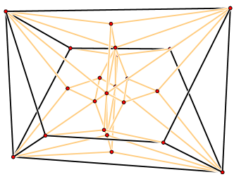
Figure 1. Schlegel diagram of the split polytope of the regular $3$-cube.

A weight function $w$ on a polytope $P$ is called split prime if for all splits $S$ of $P$ we have $\alpha^{w}_{w_{S}}=0$. The following can be seen as a generalization of Bandelt and Dress [2, Theorem 3], and as a reformulation of Hirai’s Theorem 2.2 [17].

Theorem 21 (Split Decomposition Theorem).

Each weight function $w$ has a coherent decomposition

(7) $$w\ =\ w_{0}+\sum_{\text{$S$ split of $P$}}\lambda_{S}w_{S}\,,$$

where $w_{0}$ is split prime, and this is unique among all coherent decompositions of $w$.

This is called the split decomposition of $w$.

Proof.

We first consider the special case where the subdivision ${\Sigma_{w}(P)}$ induced by $w$ is a common refinement of splits. Then each face $F$ of codimension $1$ in ${\Sigma_{w}(P)}$ defines a unique split $S(F)$, namely the one with split hyperplane $H_{S(F)}=\operatorname{lin}F$. Moreover, whenever $S$ is an arbitrary split of $P$ then $\alpha^{w}_{w_{S}}>0$ if and only if $H_{S}\cap P$ is a face of $\Delta_{w}$ of codimension $1$. This gives a coherent subdivision $w=\sum_{S}\alpha^{w}_{w_{S}}w_{S}$, where the sum ranges over all splits $S$ of $P$. Note that the uniqueness follows from the fact that for each codimension-$1$-faces of $\Delta_{w}$ there is a unique split which coarsens it.

For the general case, we let

$$w_{0}\ :=\ w-\sum_{\text{$S$ split of $P$}}\alpha^{w}_{w_{S}}w_{S}\,.$$

By construction, $w_{0}$ is split prime, and the uniqueness of the split decomposition of $w$ follows from the uniqueness of the split decomposition of $w-w_{0}$. ∎

In fact, the sum in (7) only runs over all splits in ${\mathscr{S}}(w):=\{w_{S}\,|\,\alpha^{w}_{w_{S}}>0\}$. The uniqueness part of the theorem gives us the following interesting corollary (see also Bandelt and Dress [2, Corollary 5], and Hirai [17, Proposition 3.6]):

Corollary 22.

For a weight function $w$ the set ${\mathscr{S}}(w)\cup\{w_{0}\}$ is linearly independent. In particular, $\#{\mathscr{S}}(w)\leq n-d-1$, if $\#{\mathscr{S}}(w)=n-d-1$ then $w_{0}=0$, and if $\#{\mathscr{S}}(w)=n-d-2$ then $w_{0}$ is a prime weight function.

Proof.

Suppose the set would be linearly dependent. This would yield a relation

$$\sum_{S\in{\mathscr{S}}}\lambda_{S}w_{S}\ =\ \lambda_{0}w_{0}+\sum_{S\in{\mathscr{S}}(w)\setminus{\mathscr{S}}}\lambda_{S}w_{S}$$

with coefficients $\lambda_{0},\lambda_{S}\geq 0$ for some ${\mathscr{S}}\subset{\mathscr{S}}(w)$. However, this contradicts the uniqueness part of Theorem 21 for the weight function $w^{\prime}:=\sum_{S\in{\mathscr{S}}}\lambda_{S}w_{S}$.

The cardinality constraints now follow from the fact that the weight functions live in ${\mathbb{R}}^{n}/S[0]\cong{\mathbb{R}}^{n-d-1}$. ∎

The next lemma is a specialization of Corollary 4 to the case of splits and their weight functions.

Lemma 23.

Let ${\mathscr{S}}$ be a set of splits for $P$. Then the following statements are equivalent.

1. The corresponding decomposition $w:=\sum_{S\in{\mathscr{S}}}w_{S}$ is coherent,

2. there exists a common refinement of all $S\in{\mathscr{S}}$ (induced by $w$),

3. there is a regular triangulation of $P$ which refines all $S\in{\mathscr{S}}$.

Instead of “set of splits” we equivalently use the term split system. A split system is called weakly compatible if one of the properties of Lemma 23 is satisfied. Moreover, two splits $S_{1}$ and $S_{2}$ such that $H_{S_{1}}\cap H_{S_{2}}$ does not meet $P$ in its interior are called compatible. This notion generalizes to arbitrary split systems in different ways: A set ${\mathscr{S}}$ of splits is called compatible if any two of its splits are compatible. It is incompatible if it is not compatible, and it is totally incompatible if any two of its splits are incompatible. It is clear that total incompatibility implies incompatibility, and that compatibility implies weak compatibility (but the converse does not hold, see Example 34).

For an arbitrary split system ${\mathscr{S}}$ we define its weight function as

$$w_{\mathscr{S}}\ :=\ \sum_{S\in{\mathscr{S}}}w_{S}\,.$$

If ${\mathscr{S}}$ is weakly compatible then ${\Sigma_{{\mathscr{S}}}(P)}:={\Sigma_{w_{\mathscr{S}}}(P)}$ is the coarsest subdivision refining all splits in ${\mathscr{S}}$. We further abbreviate ${{\mathscr{E}}_{{\mathscr{S}}}(P)}:={{\mathscr{E}}_{w_{\mathscr{S}}}(P)}$ and ${{\mathscr{T}}_{{\mathscr{S}}}(P)}:={{\mathscr{T}}_{w_{\mathscr{S}}}(P)}$.

Remark 24.

The split decomposition (7) of a weight function $w$ of the $d$-polytope $P$ can actually be computed using our formula (2). Provided we already know the, say, $t$ vertices of the tight span of $w$ and the, say, $s$ splits of $P$, this takes $O(s\,t\,d\,n)$ arithmetic operations over the reals (or the rationals), where $n=\#\operatorname{Vert}{P}$.

4. Split Complexes and Split Subdivisions

Let $P$ be a fixed $d$-polytope, and let ${\mathscr{S}}(P)$ be the set of all splits of $P$. The notions of compatibility and weak compatibility of splits give rise to two abstract simplicial complexes with vertex set ${\mathscr{S}}(P)$. We denote them by ${\rm Split}(P)$ and ${\rm Split}^{\rm w}(P)$, respectively. Since compatibility implies weak compatibility ${\rm Split}(P)$ is a subcomplex of ${\rm Split}^{\rm w}(P)$. Moreover, if ${\mathscr{S}}\subseteq{\mathscr{S}}(P)$ is a split system such that any two splits in ${\mathscr{S}}$ are compatible then the whole split system ${\mathscr{S}}$ is compatible. This can also be phrased in graph theory language: The compatibility relation among the splits defines an undirected graph, whose cliques correspond to the faces of ${\rm Split}(P)$. In particular, we have the following:

Proposition 25.

The split complex ${\rm Split}(P)$ is a flag simplicial complex.

Note that we did not assume that $P$ admits any split. If $P$ is unsplittable then the (weak) split complex of $P$ is the void complex $\emptyset$.

Theorem 21 tells us that the fan spanned by the rays that induce splits is a simplicial fan contained in (the support of) ${\rm SecFan}(P)$. This fan was called the split fan of $P$ by Koichi [26]. Denoting by ${\rm SecFan}^{\prime}(P)$ the (spherical) polytopal complex which arises from ${\rm SecFan}(P)$ by intersecting with the unit sphere, this leads to the following observation:

Corollary 26.

The simplicial complex ${\rm Split}(P)$ is a subcomplex of the polytopal complex ${\rm SecFan}^{\prime}(P)$.

Proof.

The tight span of a compatible system ${\mathscr{S}}$ of splits of $P$ is a tree by Proposition 30. This implies that the cell $C$ in ${\rm SecFan}^{\prime}(P)$ generated by ${\mathscr{S}}$ does not contain vertices whose tight span is of dimension greater than one. Thus the vertices of $C$ are precisely the splits in ${\mathscr{S}}$. ∎

Remark 27.

The weak split complex of $P$ is usually not a subcomplex of ${\rm SecFan}^{\prime}(P)$; see Example 34. However, one can show that ${\rm Split}^{\rm w}(P)$ is homotopy equivalent to a subcomplex of ${\rm SecFan}^{\prime}(P)$.

From Corollary 22 we can trivially derive an upper bound on the dimensions of the split complex and the weak split complex. This bound is sharp for both types of complexes as we will see in Example 32 below.

Proposition 28.

The dimensions of ${\rm Split}(P)$ and ${\rm Split}^{\rm w}(P)$ are bounded from above by $n-d-2$.

A regular subdivision (triangulation) $\Delta$ of $P$ is called a split subdivision (triangulation) if it is the common refinement of a set ${\mathscr{S}}$ of splits of $P$. Necessarily, the split system ${\mathscr{S}}$ is weakly compatible, and ${\mathscr{S}}$ is a face of ${\rm Split}^{\rm w}(P)$. Conversely, all faces of ${\rm Split}^{\rm w}(P)$ arise in this way.

Corollary 29.

If ${\mathscr{S}}$ is a facet of ${\rm Split}^{\rm w}(P)$ with $\#{\mathscr{S}}=n-d-1$ then the split subdivision ${\Sigma_{{\mathscr{S}}}(P)}$ is a split triangulation.

Proof.

Corollary 22 implies that $W:=\{w_{S}\,|\,S\in{\mathscr{S}}\}$ is linearly independent and hence a basis of ${\mathbb{R}}^{n}/S[0]\cong{\mathbb{R}}^{n-d-1}$. So the cone spanned by $W$ is full-dimensional and hence corresponds to a vertex of the secondary polytope. ∎

The following is a characterization of the faces of ${\rm Split}(P)$, and it says that split complexes are always “spaces of trees”.

Proposition 30 (Hirai [17], Proposition 2.9).

Let ${\mathscr{S}}$ be a split system on $P$. Then the following statements are equivalent.

1. ${\mathscr{S}}$ is compatible,

2. ${{\mathscr{T}}_{{\mathscr{S}}}(P)}$ is $1$-dimensional, and

3. ${{\mathscr{T}}_{{\mathscr{S}}}(P)}$ is a tree.

Proof.

Assume that ${\Sigma_{\S}(P)}$ is induced by the compatible split system ${\mathscr{S}}\neq\emptyset$. By definition, for any two distinct splits $S_{1},S_{2}\in{\mathscr{S}}$ the hyperplanes $H_{S_{1}}$ and $H_{S_{2}}$ do not meet in the interior of $P$. This implies that there are no interior faces in ${\Sigma_{\S}(P)}$ of codimension greater than $1$. By Proposition 3, this says that $\dim{{\mathscr{T}}_{\S}(P)}\leq 1$. Since ${\mathscr{S}}\neq\emptyset$ we have that $\dim{{\mathscr{T}}_{\S}(P)}=1$. Thus (i) implies (ii).

The statement (iii) follows from (ii) as the tight span is contractible.

Suppose that ${{\mathscr{T}}_{\S}(P)}$ is a tree. Then each edge is dual to a split hyperplane. The system ${\mathscr{S}}$ of all these splits is clearly weakly compatible since it is refined by ${\Sigma_{\S}(P)}$. Assume that there are splits $S_{1},S_{2}\in{\mathscr{S}}$ such that the corresponding split hyperplanes $H_{S_{1}}$ and $H_{S_{2}}$ meet in the interior of $P$. Then $H_{S_{1}}\cap H_{S_{2}}$ is an interior face in ${\Sigma_{\S}(P)}$ of codimension $2$, contradicting our assumption that ${{\mathscr{T}}_{\S}(P)}$ is a tree. This proves (i), and hence the claim follows. ∎

Remark 31.

A $d$-dimensional polytope is called stacked if it has a triangulation in which there are no interior faces of dimension less than $d-1$. So it follows from Proposition 30 that a polytope is stacked if and only if there exists a split triangulation induced by a compatible system of splits.

Example 32.

Let $P$ be a an $n$-gon for $n\geq 4$. As already pointed out in Example 18, each pair of non-neighboring vertices defines a split of $P$. Two such splits are compatible if and only if they are weakly compatible.

The secondary polytope of $P$ is the associahedron $\operatorname{Assoc}_{n-3}$, and the split complex of $P$ is isomorphic to the boundary complex of its dual. In particular, ${\rm Split}(P)={\rm Split}^{\rm w}(P)$ is a pure and shellable simplicial complex of dimension $n-4$, which is homeomorphic to ${\mathbb{S}}^{n-4}$. This shows that the bound in Proposition 28 is sharp. From Catalan combinatorics it is known that the (split) triangulations of $P$ correspond to the binary trees on $n-2$ nodes; see [7, Section 1.1].

Example 33.

The splits of the regular cross polytope $X_{d}=\operatorname{conv}\{\pm e_{1},\pm e_{2},\dots,\pm e_{d}\}$ in ${\mathbb{R}}^{d}$ are induced by the $d$ reflection hyperplanes $x_{i}=0$. Any $d-1$ of them are weakly compatible and define a triangulation of $X_{d}$ by Corollary 29. (Of course, this can also be seen directly.) All triangulations of $X_{d}$ arise in this way. This shows that ${\rm Split}^{\rm w}(X_{d})$ is isomorphic to the boundary complex of a $(d-1)$-dimensional simplex, which is also the secondary polytope and the split polytope of $X_{d}$. Any two reflection hyperplanes meet in the interior of $X_{d}$, whence no two splits are compatible. This says that ${\rm Split}(X_{d})$ consists of $d$ isolated points.

Example 34.

As we already discussed in Example 19 the regular $3$-cube $C_{3}=[-1,1]^{3}$ has a total number of $14$ splits. The split complex ${\rm Split}(C)$ is $3$-dimensional but not pure; its $f$-vector reads $(14,40,32,2)$. The two $3$-dimensional facets correspond to the two non-unimodular triangulations of $C$ (arising from splitting every other vertex). The reduced homology is concentrated in dimension two, and we have $H_{2}({\rm Split}(C_{3});{\mathbb{Z}})\cong{\mathbb{Z}}^{3}$. The graph indicating the compatibility relation among the splits is shown in Figure 2.

Figure 3 shows three triangulations of $C_{3}$. The left one is generated by a totally incompatible system of three splits; that is, it is a facet of ${\rm Split}^{\rm w}(C_{3})$ which is not a face of ${\rm Split}(C_{3})$. The right one is (not unimodular and) generated by a compatible split system (of four vertex splits); that is, it is a facet of both ${\rm Split}(C_{3})$ and ${\rm Split}^{\rm w}(C_{3})$. The middle one is not generated by splits at all.

The triangulation $\Delta$ on the left uses only three splits. This examples shows that the converse of Corollary 29 is not true, that is, a weakly compatible split system that defines a triangulation does not have to be maximal with respect to cardinality. Furthermore, the triangulation $\Delta$ can also be obtained as the common refinement of two non-split coarsest subdivisions. The cell in ${\rm SecFan}^{\prime}(C_{3})$ corresponding to $\Delta$ is a bipyramid over a triangle. The vertices of this triangle (which is not a face of ${\rm SecFan}^{\prime}(C_{3})$) correspond to the three splits, so the relevant cell in ${\rm Split}^{\rm w}(C_{3})$ is a triangle, and the apices corresponds to the non-split coarsest subdivisions mentioned above. Since the three splits are totally incompatible there does not exist a corresponding face in ${\rm Split}(C_{3})$, and the intersection with ${\rm Split}(C_{3})$ consists of three isolated points.

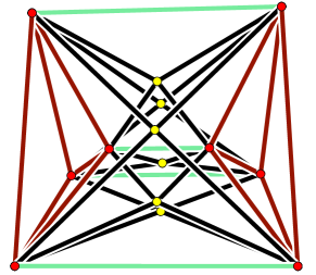
Figure 2. Compatibility graph of the splits of the regular $3$-cube. The four (red) nodes to the left and the four (red) nodes to the right correspond to the vertex splits.

A polytopal complex is zonotopal if each face is zonotope. A zonotope is the Minkowski sum of line segments or, equivalently, the affine projection of a regular cube. Any graph, that is, a $1$-dimensional polytopal complex, is zonotopal in a trivial way. So especially tight spans of splits and, by Proposition 30, of compatible splits systems are zonotopal. In fact, this is even true for arbitrary weakly compatible splits systems. See also Bolker [5, Theorem 6.11] and Hirai [17, Corollary 2.8].

Theorem 35.

Let ${\mathscr{S}}$ be a weakly compatible split system on $P$. Then the tight span ${{\mathscr{T}}_{{\mathscr{S}}}(P)}$ is a (not necessarily pure) zonotopal complex.

Proof.

Let $F$ be a face of ${{\mathscr{T}}_{{\mathscr{S}}}(P)}$. Since by Lemma 23 we have that ${{\mathscr{E}}_{{\mathscr{S}}}(P)}=\sum_{S\in{\mathscr{S}}}{{\mathscr{E}}_{w_{S}}(P)}$ we get (by the same arguments used in the proof of Lemma 2) that $F=\sum_{S\in{\mathscr{S}}}F_{S}$ for faces $F_{S}$ of ${{\mathscr{T}}_{w_{S}}(P)}$. The claim now follows from the fact that ${{\mathscr{T}}_{w_{S}}(P)}$ is a line segment for all $S\in{\mathscr{S}}$. ∎

A triangulation of a $d$-polytope is foldable if its vertices can be colored with $d$ colors such that each edge of the triangulation receives two distinct colors. This is equivalent to requiring that the dual graph of the triangulation is bipartite; see [22, Corollary 11]. Note that foldable simplicial complexes are called “balanced” in [22]. The three triangulations of the regular $3$-cube in Figure 3 are foldable.

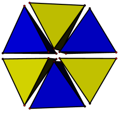
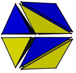
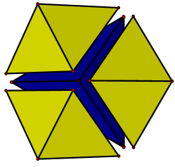
Figure 3. Three foldable triangulations of the regular $3$-cube.

Corollary 36.

Each split triangulation is foldable.

Proof.

Let ${\mathscr{S}}$ be a weakly compatible split system such that ${\Sigma_{{\mathscr{S}}}(P)}$ is a triangulation. By Theorem 35 each $2$-dimensional face of the tight span ${{\mathscr{T}}_{{\mathscr{S}}}(P)}$ has an even number of vertices. This implies that ${\Sigma_{{\mathscr{S}}}(P)}$ is a triangulation of $P$ such that each of its interior codimension-$2$-cell is contained in an even number of maximal cells. Now the claim follows from [22, Corollary 11]. ∎

Example 37.

Let $C_{4}$ be the $4$-dimensional cube. In Figure 4 there is a picture of the tight span ${{\mathscr{T}}_{{\mathscr{S}}}(C_{4})}$ of a split system ${\mathscr{S}}$ of $C_{4}$ with 10 weakly compatible splits. As proposed by Theorem 35 the complex is zonotopal. It is $3$-dimensional and its $f$-vector reads $(24,36,14,1)$. The number of vertices equals $24=4!$ which is the normalized volume of $C_{4}$, and hence ${\Sigma_{{\mathscr{S}}}(C_{4})}$ is, in fact, a triangulation. By Corollary 36 this triangulation is foldable.

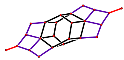
Figure 4. The tight span of a split triangulation of the $4$-cube.

5. Hypersimplices

As a notational shorthand we abbreviate $[n]:=\{1,2,\dots,n\}$ and $\binom{[n]}{k}:=\{X\subseteq[n]\,|\,\#X=k\}$. The $k$-th hypersimplex in ${\mathbb{R}}^{n}$ is defined as

$${\Delta(k,n)}\ :=\ \left\{x\in[0,1]^{n}\vphantom{\sum_{i=1}^{n}x_{i}=k}\,\right.\left|\,\vphantom{x\in[0,1]^{n}}\sum_{i=1}^{n}x_{i}=k\right\}\ =\ \operatorname{conv}\left\{\sum_{i\in A}e_{i}\vphantom{A\in\binom{[n]}{k}}\,\right.\left|\,\vphantom{\sum_{i\in A}e_{i}}A\in\binom{[n]}{k}\right\}\,.$$

It is $(n-1)$-dimensional and satisfies the conditions of Section 2. Throughout the following we assume that $n\geq 2$ and $1\leq k\leq n-1$.

A hypersimplex ${\Delta(1,n)}$ is an $(n-1)$-dimensional simplex. For arbitrary $k\geq 1$ we have ${\Delta(k,n)}\cong{\Delta(n-k,n)}$. Moreover, for $p\in[n]$ the equation $x_{p}=0$ defines a facet isomorphic to ${\Delta(k,n-1)}$. And, if $k\geq 2$, the equation $x_{p}=1$ defines a facet isomorphic to ${\Delta(k-1,n)}$. This list of facets (induced by the facets of $[0,1]^{n}$) is exhaustive. Since the hypersimplices are not full-dimensional, the facet defining (affine) hyperplanes are not unique. For the following it will be convenient to work with linear hyperplanes. This way $x_{p}=1$ gets replaced by

(8) $$(k-1)x_{p}\ =\ \sum_{i\in[n]\setminus\{p\}}x_{i}\,.$$

The triplet $(A,B;\mu)$ with $\emptyset\neq A,B\subsetneq[n]$, $A\cup B=[n]$, $A\cap B=\emptyset$ and $\mu\in{\mathbb{N}}$ defines the linear equation

(9) $$\mu\sum_{i\in A}x_{i}\ =\ (k-\mu)\sum_{i\in B}x_{i}\,.$$

The corresponding (linear) hyperplane in ${\mathbb{R}}^{n}$ is called the $(A,B;\mu)$-hyperplane. Clearly, $(A,B;\mu)$ and $(B,A;k-\mu)$ define the same hyperplane. The Equation (8) corresponds to the $(\{p\},[n]\setminus\{p\};k-1)$-hyperplane.

Lemma 38.

The $(A,B;\mu)$-hyperplane is a split hyperplane of ${\Delta(k,n)}$ if and only if $k-\mu+1\leq\#A\leq n-\mu-1$ and $1\leq\mu\leq k-1$.

Proof.

It is clear that the $(A,B;\mu)$-hyperplane does not meet the interior of ${\Delta(k,n)}$ if $\mu\leq 0$ or if $\mu\geq k$. Especially, we may assume that $k\geq 2$.

Suppose now that $\#A\leq k-\mu$. Then each point $x\in{\Delta(k,n)}$ satisfies $\sum_{i\in A}x_{i}\leq k-\mu$ and $\sum_{i\in B}x_{i}\geq k-(k-\mu)=\mu$. This implies that $\mu\sum_{i\in A}x_{i}\leq(k-\mu)\sum_{i\in B}x_{i}$, which says that all points in ${\Delta(k,n)}$ are contained in one of the two halfspaces defined by the $(A,B;\mu)$-hyperplane. Hence it does not define a split. A similar argument shows that $\#A\leq n-\mu-1$ is necessary in order to define a split.

Conversely, assume that $k-\mu+1\leq\#A\leq n-\mu-1$ and $1\leq\mu\leq k-1$. We define a point $x\in{\Delta(k,n)}$ by setting

$$x_{i}\ :=\ \begin{cases}\frac{k-\mu}{\#A}&\text{if $i\in A$}\\ \frac{\mu}{\#B}&\text{if $i\in B$}\,.\end{cases}$$

Since $0<\frac{k-\mu}{\#A}<1$ and $0<\frac{\mu}{\#B}<1$ the point $x$ is contained in the (relative) interior of ${\Delta(k,n)}$. Moreover, $x$ satisfies the Equation (9), and so the $(A,B;\mu)$-hyperplane passes through the interior of ${\Delta(k,n)}$.

It remains to show that the $(A,B;\mu)$-hyperplane does not separate any edge. Let $v$ and $w$ be two adjacent vertices. So we have some $\{p,q\}\in\tbinom{[n]}{2}$ with $v-w=e_{p}-e_{q}$. Aiming at an indirect argument, we assume that $v$ and $w$ are on opposite sides of the $(A,B;\mu)$-hyperplane, that is, without loss of generality $\mu\sum_{i\in A}v_{i}>(k-\mu)\sum_{i\in B}v_{i}$ and $\mu\sum_{i\in A}w_{i}<(k-\mu)\sum_{i\in B}w_{i}$. This gives

$$0\ <\ \mu\sum_{i\in A}v_{i}\,-\,(k-\mu)\sum_{i\in B}v_{i}\ =\ \mu(\chi_{A}(p)-\chi_{A}(q))$$

and

$$0\ <\ (k-\mu)\sum_{i\in B}w_{i}\,-\,\mu\sum_{i\in A}w_{i}\ =\ (k-\mu)(\chi_{B}(p)-\chi_{B}(q))\,,$$

where characteristic functions are denoted as $\chi_{\cdot}(\cdot)$. Since $\mu>0$ and $\mu<k$ it follows that $\chi_{A}(q)<\chi_{A}(p)$ and $\chi_{B}(q)<\chi_{B}(p)$. Now the characteristic functions take values in $\{0,1\}$ only, and we arrive at $\chi_{A}(q)=\chi_{B}(q)=0$ and $\chi_{A}(p)=\chi_{B}(p)=1$. Both these equations contradict the fact that $(A,B)$ is a partition of $[n]$. So we conclude that, indeed, the $(A,B;\mu)$-hyperplane defines a split. ∎

This allows to characterize the splits of the hypersimplices.

Proposition 39.

Each split hyperplane of ${\Delta(k,n)}$ is defined by a linear equation of the type (9).

Proof.

Using Observation 12 and exploiting the fact that facets of hypersimplices are hypersimplices we can proceed by induction on $n$ and $k$ as follows.

Our induction is based on the case $k=1$. Since ${\Delta(1,n)}$ is an $(n-1)$-simplex, which does not have any splits, the claim is trivially satisfied. The same holds for $k=n-1$ as ${\Delta(n-1,n)}\cong{\Delta(1,n)}$.

For the rest of the proof we assume that $2\leq k\leq n-2$. In particular, this implies that $n\geq 4$.

Let $\sum_{i\in[n]}\alpha_{i}x_{i}=0$ define a split hyperplane $H$ of ${\Delta(k,n)}$. The facet defining hyperplane $F_{p}=\{x\,|\,x_{p}=0\}$ is intersected by $H$, and we have

$$F_{p}\cap H\ =\ \biggl{\{}x\in{\mathbb{R}}^{n}\,\biggl{|}\,\sum_{i\in[n]\setminus\{p\}}\alpha_{i}x_{i}=0=x_{p}\biggr{\}}\,.$$

Three cases arise:

1. $F_{p}\cap H$ is a facet of $F_{p}\cap{\Delta(k,n)}\cong{\Delta(k,n-1)}$ defined by $x_{q}=0$ (with $q\neq p$),

2. $F_{p}\cap H$ is a facet of $F_{p}\cap{\Delta(k,n)}\cong{\Delta(k,n-1)}$ as defined by Equation (8), or

3. $F_{p}\cap H$ defines a split of $F_{p}\cap{\Delta(k,n)}\cong{\Delta(k,n-1)}$.

If $F_{p}\cap H$ is of type (i) then it follows that $\alpha_{i}=0$ for all $i\neq p$ and $\alpha_{p}\neq 0$. As not all the $\alpha_{i}$ can vanish there is at most one $p\in[n]$ such that $F_{p}\cap H$ is of type (i). Since we could assume that $n\geq 4$ there are at least two distinct $p,q\in[n]$ such that $F_{p}\cap H$ and $F_{q}\cap H$ are of type (ii) or (iii). By symmetry, we can further assume that $p=1$ and $q=n$. So we get a partition $(A,B)$ of $[n-1]$ and a partition $(A^{\prime},B^{\prime})$ of $\{2,3,\dots,n\}$ with $\mu,\mu^{\prime}\in{\mathbb{N}}$ such that $F_{1}\cap H$ is defined by $x_{1}=0$ and

$$\mu\sum_{i\in A}x_{i}\ =\ (k-\mu)\sum_{i\in B}x_{i}\,,$$

while $F_{n}\cap H$ is defined by $x_{n}=0$ and

$$\mu^{\prime}\sum_{i\in A^{\prime}}x_{i}\ =\ (k-\mu^{\prime})\sum_{i\in B^{\prime}}x_{i}\,.$$

We infer that there is a real number $\lambda$ such that $\alpha_{i}=\lambda\mu$ for all $i\in A$, $\alpha_{i}=\lambda(k-\mu)$ for all $i\in B$. It remains to show that $\alpha_{n}\in\{\lambda\mu,\lambda(k-\mu)\}$. Similarly, there is a real number $\lambda^{\prime}$ such that $\alpha_{i}=\lambda^{\prime}\mu^{\prime}$ for all $i\in A^{\prime}$, $\alpha_{i}=\lambda^{\prime}(k-\mu^{\prime})$ for all $i\in B^{\prime}$. As $n\geq 4$ we have $A\cap A^{\prime}\neq\emptyset$ or $B\cap B^{\prime}\neq\emptyset$. We obtain $\alpha_{i}=\lambda\mu=\lambda^{\prime}\mu^{\prime}$ for $i\in(A\cap A^{\prime})\cup(B\cap B^{\prime})$. Finally, this shows that $\alpha_{n}\in\{\lambda^{\prime}\mu^{\prime},\lambda^{\prime}(k-\mu^{\prime})\}=\{\lambda\mu,\lambda(k-\mu)\}$, and this completes the proof. ∎

Theorem 40.

The total number of splits of the hypersimplex ${\Delta(k,n)}$ (with $k\leq n/2$) equals

$$\ (k-1)\left(2^{n-1}-(n+1)\right)-\sum_{i=2}^{k-1}(k-i)\binom{n}{i}\;.$$

Proof.

We have to count the $(A,B;\mu)$-hyperplanes with the restrictions listed in Lemma 38. So we take a set $A\subset[n]$ with at least 2 and at most $n-2$ elements. If $A$ has cardinality $i$ then there are $\min(k-1,n-i-1)-\max(1,k-i+1)+1$ choices for $\mu$. Recall that $(A,B;\mu)$ and $(B,A;k-\mu)$ define the same split; in this way we have counted each split twice. So we get

$$\frac{1}{2}\sum_{i=2}^{n-2}\big{(}\min(k,n-i)-\max(1,k-i+1)\big{)}\binom{n}{i}\ =\ \frac{1}{2}\sum_{i=2}^{n-2}\big{(}\min(i,k,n-i)-1\big{)}\binom{n}{i}$$

splits, where the equality holds since $k\leq n/2$. For a further simplification we rewrite the sum to get

$$\begin{split}\frac{1}{2}\sum_{i=2}^{k-1}&(i-1)\binom{n}{i}+\frac{1}{2}\sum_{i=k}^{n-k}(k-1)\binom{n}{i}+\frac{1}{2}\sum_{i=n-k+1}^{n-2}(n-i-1)\binom{n}{i}\\ &=\ \frac{1}{2}(k-1)\sum_{i=2}^{n-2}\binom{n}{i}+\frac{1}{2}\sum_{i=2}^{k-1}\big{(}i-1-(k-1)\big{)}\binom{n}{i}+\frac{1}{2}\sum_{i=n-k+1}^{n-2}\big{(}n-i-1-(k-1)\big{)}\binom{n}{i}\\ &=\ (k-1)\left(2^{n-1}-(n+1)\right)-\sum_{i=2}^{k-1}(k-i)\binom{n}{i}\,.\end{split}$$

∎

If we have two distinct splits $(A,B;\mu)$ and $(C,D;\nu)$ then either $\{A\cap C,A\cap D,B\cap C,B\cap D\}$ is a partition of $[n]$ into four parts, or exactly one of the four intersections is empty. If, for instance, $B\cap D=\emptyset$ then $B\subseteq C$ and $D\subseteq A$.

Proposition 41.

Two splits $(A,B;\mu)$ and $(C,D;\nu)$ of ${\Delta(k,n)}$ are compatible if and only if one of the following holds:

$$\#(A\cap C)\ \leq\ k-\mu-\nu\,, \#(A\cap D)\ \leq\ \nu-\mu\,,$$

$$\#(B\cap C)\ \leq\ \mu-\nu\,, \text{or }\quad\#(B\cap D)\ \leq\ \mu+\nu-k\,.$$

For an arbitrary set $I\subseteq[n]$ we abbreviate $x_{I}:=\sum_{i\in I}x_{i}$. In particular, $x_{\emptyset}=0$ and for $x\in{\Delta(k,n)}$ one has $x_{[n]}=k$.

Proof.

Let $x\in{\Delta(k,n)}$ be in the intersection of the $(A,B;\mu)$-hyperplane and the $(C,D;\nu)$-hyperplane. Our split equations take the form

$$\mu(x_{A\cap C}+x_{A\cap D})\ =\ (k-\mu)(x_{B\cap C}+x_{B\cap D})\quad\text{and}$$

$$\nu(x_{A\cap C}+x_{B\cap C})\ =\ (k-\nu)(x_{A\cap D}+x_{B\cap D})\,.$$

In view of $(A\cap C)\cup(A\cap D)\cup(B\cap C)\cup(B\cap D)=[n]$ we additionally have $x_{A\cap C}+x_{A\cap D}+x_{B\cap C}+x_{B\cap D}=k$, and thus we arrive at the equivalent system of linear equations

(10) $$x_{A\cap C}\ =\ k-\mu-\nu+x_{B\cap D}\,,\quad x_{A\cap D}\ =\ \nu-x_{B\cap D}\,,\quad\text{and}\quad x_{B\cap C}\ =\ \mu-x_{B\cap D}$$

from which we can further derive

(11) $$x_{A}\ =\ k-\mu\,,\quad x_{B}\ =\ \mu\,,\quad x_{C}\ =\ k-\nu\,,\quad\text{and}\quad x_{D}\ =\ \nu\,.$$

Now the two given splits are incompatible if and only if there exists a point $x\in(0,1)^{n}$ satisfying the conditions (10).

Suppose first that none of the four intersections $A\cap C$, $A\cap D$, $B\cap C$, and $B\cap D$ is empty. Then $x\in(0,1)^{n}$ satisfies the Equations (10) if and only if the system of inequalities in $x_{B\cap D}$

(16) $$\begin{array}[]{lclcl}0&<&x_{B\cap D}&<&\#(B\cap D)\\ 0&<&k-\mu-\nu+x_{B\cap D}&<&\#(A\cap C)\\ 0&<&\mu-x_{B\cap D}&<&\#(B\cap C)\\ 0&<&\nu-x_{B\cap D}&<&\#(A\cap D)\end{array}$$

has a solution. This is equivalent to the following system of inequalities:

$$\begin{array}[]{lclcl}0&<&x_{B\cap D}&<&\#(B\cap D)\\ \mu+\nu-k&<&x_{B\cap D}&<&\#(A\cap C)+\mu+\nu-k\\ \mu-\#(B\cap C)&<&x_{B\cap D}&<&\mu\\ \nu-\#(A\cap D)&<&x_{B\cap D}&<&\nu\,.\end{array}$$

Obviously, the latter system admits a solution if and only if each of the four terms on the left is smaller than each of the four terms on the right. Most of the resulting 16 inequalities are redundant. The following four inequalities remain

$$\#(A\cap C)\ >\ k-\mu-\nu$$

$$\#(A\cap D)\ >\ \nu-\mu$$

$$\#(B\cap C)\ >\ \mu-\nu$$

$$\#(B\cap D)\ >\ \mu+\nu-k\,,$$

and this completes the proof of this case.

For the remaining cases, we can assume by symmetry that $A\cap C=\emptyset$. Then $x\in(0,1)^{n}$ satisfies the Equations (10) if and only if $x_{B\cap D}=\mu+nu=-k$, $x_{A\cap D}=k-\mu$, and $x_{B\cap C}=k-\nu$. So the splits are not compatible if and only if

$$\begin{array}[]{lclcl}0&<&k-\mu&<&\#(A\cap D)=\#A\\ 0&<&k-\nu&<&\#(B\cap C)=\#C\\ 0&<&\mu+\nu-k&<&\#(B\cap D)\,.\end{array}$$

Since, by Lemma 38, the first two inequalities hold for all splits this proves that the splits are compatible if and only if

$$\#(A\cap C)=0\leq k-\mu-\nu\quad\text{or}\quad\#(B\cap D)\leq\mu+nu-k.$$

However, again by using Lemma 38, one has $\#(A\cap D)=\#A>k-\mu>\nu-\mu$, so $\#(A\cap D)\leq\nu-\mu$ and, similarly, $\#(B\cap C)\leq\mu-\nu$ cannot be true. This completes the proof. ∎

In fact, the four cases of the proposition are equivalent in the sense that, by renaming the four sets and exchanging $\mu$ and $\nu$ or $\mu$ and $k-\mu$ in a suitable way, one will always be in the first case.

Example 42.

We consider the case $k=3$ and $n=6$. For instance, the splits $(\{1,2,6\},\{3,4,5\};2)$ and $(\{4,5,6\},\{1,2,3\};2)$ are compatible since the intersection $\{3,4,5\}\cap\{1,2,3\}=\{3\}$ has only one element and $2+2-3=1$, that is, the inequality “$\#(C\cap D)\leq\mu+\nu-k$” is satisfied.

Corollary 43.

Two splits $(A,B;\mu)$ and $(A,B;\nu)$ of ${\Delta(k,n)}$ are always compatible.

Proof.

Without loss of generality we can assume that $\mu\geq\nu$. Then the condition “$\#(B\cap C)\leq\mu-\nu$” of Proposition 41 is satisfied. ∎

In Proposition 56 below we will show that the $1$-skeleton of the weak split complex of any hypersimplex is always a complete graph. In particular, the weak split complex of ${\Delta(k,n)}$ is connected. (Or it is void if $k\in\{1,n-1\}$.)

6. Finite Metric Spaces

This section revisits the classical case, studied in the papers by Bandelt and Dress [1, 2]; see also Isbell [20]. Its purpose is to show how some of the key results can be obtained as immediate corollaries to our results above.

Let $\delta:\tbinom{[n]}{2}\to{{\mathbb{R}}_{\geq 0}}$ be a metric on the finite set $[n]$; that is, $\delta$ is a symmetric dissimilarity function which obeys the triangle inequality. By setting

$$w_{\delta}(e_{i}+e_{j})\ :=\ -\delta(i,j)$$

each metric $\delta$ defines a weight function $w_{\delta}$ on the second hypersimplex ${\Delta(2,n)}$. Hence the results for $k=2$ from Section 5 can be applied here. The tight span of $\delta$ is the tight span ${{\mathscr{T}}_{w_{\delta}}({\Delta(2,n)})}$.

Let $S=(A,B)$ be a split partition of the set $[n]$, that is, $A,B\subseteq[n]$ with $A\cup B=[n]$, $A\cap B=\emptyset$, $\#A\geq 2$, and $\#B\geq 2$. This gives rise to the split metric

$$\delta_{S}(i,j)\ :=\ \begin{cases}0&\text{if $\{i,j\}\subseteq A$ or $\{i,j\}\subseteq B$,}\\ 1&\text{otherwise.}\end{cases}$$

The weight function $w_{\delta_{S}}=-\delta_{S}$ induces a split of the second hypersimplex ${\Delta(2,n)}$, which is induced by the $(A,B;1)$-hyperplane defined in Equation (9). Proposition 39 now implies the following characterization.

Corollary 44.

Each split of ${\Delta(2,n)}$ is induced by a split metric.

Specializing the formula in Theorem 40 with $k=2$ gives the following.

Corollary 45.

The total number of splits of the hypersimplex ${\Delta(2,n)}$ equals $2^{n-1}-n-1$.

The following corollary and proposition shows that our notions of compatibility and weak compatibility agree with those of Bandelt and Dress [2] for in the special case of ${\Delta(2,n)}$.

Corollary 46 (Hirai [17], Proposition 4.16).

Two splits $(A,B)$ and $(C,D)$ of ${\Delta(2,n)}$ are compatible if and only if one of the four sets $A\cap C$, $A\cap D$, $B\cap C$, and $B\cap D$ is empty.

Proof.

Let $(A,B)$ and $(C,D)$ be splits of ${\Delta(2,n)}$. We are in the situation of Proposition 41 with $k=2$ and $\mu=\nu=1$. Hence all the right hand sides of the four inequalities in Proposition 41 yield zero, and this gives the claim. ∎

For a splits $S=(A,B)$ of ${\Delta(2,n)}$ and $m\in[n]$ we denote by $S(m)$ that of the two set $A$, $B$ with $m\in S(m)$.

Proposition 47.

A set ${\mathscr{S}}$ of splits of ${\Delta(2,n)}$ is weakly compatible if and only if there does not exist $m_{0},m_{1},m_{2},m_{3}\in[n]$ and $S_{1},S_{2},S_{3}\in{\mathscr{S}}$ such that $m_{i}\in S_{j}$ if and only if $i=j$.

Proof.

This is the definition of a weakly compatible split system ${\Delta(2,n)}$ originally given by Bandelt and Dress in [2, Section 1, page 52]. Their Corollary 10 states that ${\mathscr{S}}$ is weakly compatible in their sense if and only if $\sum_{S\in{\mathscr{S}}}w_{S}$ is a coherent decomposition. However, this is our definition of weakly compatibility according to Lemma 23. ∎

Example 48.

The hypersimplex ${\Delta(2,4)}$ is the regular octahedron, already studied in Example 33. It has the three splits $(\{1,2\},\{3,4\})$, $(\{1,3\},\{2,4\})$, and $(\{1,4\},\{2,3\})$. The weak split complex is a triangle, and the split compatibility graph consists of three isolated points.

The split compatibility graph of ${\Delta(2,5)}$ is isomorphic to the Petersen graph. It is shown in Figure 5.

Figure 5. Split compatibility graph of ${\Delta(2,5)}$; a split $(A,B)$ with $1\in A$ is labeled “$A$”.

By Proposition 30 each compatible system of splits gives rise to a tree. On the other hand, given a tree with $n$ labeled leaves take for each edge $E$ that is not connected to a leave the split $(A,B)$ where $A$ is the set of labels on one side of $E$ and $B$ the set of labels on the other side. So each tree gives rise to a system of splits for ${\Delta(2,k)}$ which is easily seen to be compatible. This argument can be augmented to a proof of the following theorem.

Theorem 49 (Buneman [6]; Billera, Holmes, and Vogtmann [3]).

The split complex ${\rm Split}({\Delta(2,n)})$ is the complex of trivalent leaf-labeled trees with $n$ leaves.

The split complex ${\rm Split}({\Delta(2,n)})$ is equal to the link of the origin $L_{n-1}$ of the space of phylogenetic trees in [3]. It was proved in [42, Theorem 2.4] (see also Robinson and Whitehouse [35]) that ${\rm Split}({\Delta(2,n)})$ is homotopy equivalent to a wedge of $n-3$ spheres. By a result of Trappmann and Ziegler, ${\rm Split}({\Delta(2,n)})$ is even shellable [41]. Markwig and Yu [31] recently identified the space of $k$ tropically collinear points in the tropical $(d-1)$-dimensional affine space as a (shellable) subcomplex of ${\rm Split}({\Delta(2,k+d)})$.

Example 50.

Consider the split system ${\mathscr{S}}=\{(A_{ij},[n]\setminus A_{ij})\,|\,1\leq i<j\leq n\text{ and }j-i<n-2\}$ where $A_{ij}:=\{i,i+1,\dots,j-1,j\}$ for the hypersimplex ${\Delta(2,n)}$. The combinatorial criterion of Proposition 47 shows that this split system is weakly compatible, and that $\#{\mathscr{S}}=\binom{n}{2}-n$. Since ${\Delta(2,n)}$ has $\binom{n}{2}$ vertices and is of dimension $n-1$, Corollary 29 implies that ${\Sigma_{{\mathscr{S}}}(P)}$ is a triangulation. This triangulation is known as the thrackle triangulation in the literature; see [8], [40, Chapter 14], and additionally [39, 2, 29, 15] for further occurrences of this triangulation. In fact, as one can conclude from [11, Theorem 3.1] in connection with [2, Theorem 5], this is the only split triangulation of ${\Delta(2,n)}$, up to symmetry.

7. Matroid Polytopes and Tropical Grassmannians

In the following, we copy some information from Speyer and Sturmfels [38]; the reader is referred to this source for the details.

Let ${\mathbb{Z}}[p]:={\mathbb{Z}}[p_{i_{1},\dots,i_{k}}\,|\,1\leq i_{1}<i_{2}<\dots<i_{k}\leq n]$ be the polynomial ring in $\tbinom{n}{k}$ indeterminates with integer coefficients. The indeterminate $p_{i_{1},\dots,i_{k}}$ can be identified with the $k\times k$-minor of a $k\times n$-matrix with columns numbered $(i_{1},i_{2},\dots,i_{k})$. The Plücker ideal $I_{k,n}$ is defined as the ideal generated by the algebraic relations among these minors. It is obviously homogeneous, and it is known to be a prime ideal. For an algebraically closed field $K$ the projective variety defined by $I_{k,n}\otimes_{\mathbb{Z}}K$ in the polynomial ring $K[p]={\mathbb{Z}}[p]\otimes_{\mathbb{Z}}K$ is the Grassmannian ${G_{k,n}}$ (over $K$). It parameterizes the $k$-dimensional linear subspaces of the vector space $K^{n}$.

For instance, we can pick $K$ as the algebraic closure of the field ${\mathbb{C}}(t)$ of rational functions. Then for an arbitrary ideal $I$ in $K[x]=K[x_{1},\dots,x_{m}]$ its tropicalization ${\mathscr{T}}(I)$ is the set of all vectors $w\in{\mathbb{R}}^{m}$ such that the initial ideal $\operatorname{in}_{w}(I)$ with respect to the term order defined by the weight function $w$ does not contain any monomial. The tropical Grassmannian ${{\mathscr{G}}_{k,n}}$ (over $K$) is the tropicalization of the Plücker ideal $I_{k,n}\otimes_{\mathbb{Z}}K$.

The tropical Grassmannian ${{\mathscr{G}}_{k,n}}$ is a polyhedral fan in ${\mathbb{R}}^{\tbinom{n}{k}}$ such that each of its maximal cones has dimension $(n-k)k+1$. In a way the fan ${{\mathscr{G}}_{k,n}}$ contains redundant information. We describe the three step reduction in [38, Section 3].

Let $\phi$ be the linear map from ${\mathbb{R}}^{n}$ to ${\mathbb{R}}^{\tbinom{n}{k}}$ which sends $x=(x_{1},\dots,x_{n})$ to $(x_{I}\,|\,I\in\tbinom{n}{k})$. Recall that $x_{I}$ is defined as $\sum_{i\in I}x_{i}$. The map $\phi$ is injective, and its image $\operatorname{im}\phi$ coincides with the intersection of all maximal cones in ${{\mathscr{G}}_{k,n}}$. Moreover, the vector $\mathbbm{1}:=(1,1,\dots,1)$ of length $\tbinom{n}{k}$ is contained in the image of $\phi$. This leads to the definition of the two quotient fans

$${{\mathscr{G}}^{\prime}_{k,n}}\ :=\ {{\mathscr{G}}_{k,n}}/{\mathbb{R}}\mathbbm{1}\quad\text{and}\quad{{\mathscr{G}}^{\prime\prime}_{k,n}}\ :=\ {{\mathscr{G}}_{k,n}}/\operatorname{im}\phi\,.$$

Finally, let ${{\mathscr{G}}^{\prime\prime\prime}_{k,n}}$ be the (spherical) polytopal complex arising from intersecting ${{\mathscr{G}}^{\prime\prime}_{k,n}}$ with the unit sphere in ${\mathbb{R}}^{\tbinom{n}{k}}/\operatorname{im}\phi$. We have $\dim{{\mathscr{G}}^{\prime\prime\prime}_{k,n}}=n(k-1)-k^{2}$. It seems to be common practice to use the name “tropical Grassmannian” interchangeably for ${{\mathscr{G}}_{k,n}}$, ${{\mathscr{G}}^{\prime}_{k,n}}$, ${{\mathscr{G}}^{\prime\prime}_{k,n}}$, as well as ${{\mathscr{G}}^{\prime\prime\prime}_{k,n}}$.

It is unlikely that it is possible to give a complete combinatorial description of all tropical Grassmannians. The contribution of combinatorics here is to provide kind of an “approximation” to the tropical Grassmannians via matroid theory. For a background on matroids, see the books edited by White [43, 44].

The tropical pre-Grassmannian ${{\rm pre-}{\mathscr{G}}_{k,n}}$ is the subfan of the secondary fan of ${\Delta(k,n)}$ of those weight functions which induce matroid subdivisions. A polytopal subdivision $\Sigma$ of ${\Delta(k,n)}$ is a matroid subdivision if each (maximal) cell is a matroid polytope. If $M$ is a matroid on the set $[n]$ then the corresponding matroid polytope is the convex hull of those $0/1$-vectors in ${\mathbb{R}}^{n}$ which are characteristic functions of the bases of $M$. A finite point set $X\subset{\mathbb{R}}^{d}$ (possibly with multiple points) gives rise to a matroid ${\mathscr{M}}(X)$ by taking as bases for ${\mathscr{M}}(X)$ the maximal affinely independent subsets of $X$. The following characterization of matroid subdivisions is essential.

Theorem 51 (Gel^′fand, Goresky, MacPherson, and Serganova [13], Theorem 4.1).

Let $\Sigma$ be a polytopal subdivision of ${\Delta(k,n)}$. The following are equivalent:

1. The maximal cells of $\Sigma$ are matroid polytopes, that is, $\Sigma$ is a matroid subdivision,

2. the $1$-skeleton of $\Sigma$ coincides with the $1$-skeleton of ${\Delta(k,n)}$, and

3. the edges in $\Sigma$ are parallel to the edges of ${\Delta(k,n)}$.

Regular matroid subdivisions of hypersimplices are called “generalized Lie complexes” by Kapranov [24]. The corresponding equivalence classes of weight functions are the “tropical Plücker vectors” of Speyer [36].

The relationship between the two fans ${{\rm pre-}{\mathscr{G}}_{k,n}}$ and ${{\mathscr{G}}_{k,n}}$ is the following. Algebraically, ${{\rm pre-}{\mathscr{G}}_{k,n}}$ is the tropicalization of the ideal of quadratic Plücker relations; see Speyer [36, Section 2]. Conversely, each weight function in the fan ${{\mathscr{G}}_{k,n}}$ gives rise to a matroid subdivision of ${\Delta(k,n)}$. However, since there is no secondary fan naturally associated with ${{\mathscr{G}}_{k,n}}$ it is a priori not clear how ${{\mathscr{G}}_{k,n}}$ sits inside ${{\rm pre-}{\mathscr{G}}_{k,n}}$. Note that, unlike ${{\mathscr{G}}_{k,n}}$, the tropical pre-Grassmannian does not depend on the characteristic of the field $K$.

Our goal for the rest of this section is to explain how the hypersimplex splits are related to the tropical (pre-)Grassmannians.

Proposition 52.

Let $\Sigma$ be a matroid subdivision and $S$ a split of ${\Delta(k,n)}$. Then $\Sigma$ and $S$ have a common refinement (without new vertices).

Proof.

Of course, one can form the common refinement $\Sigma^{\prime}$ of $\Sigma$ and $S$ but $\Sigma^{\prime}$ may contain additional vertices, and hence does not have to be a polytopal subdivision of ${\Delta(k,n)}$. However, additional vertices can only occur if some edge of $\Sigma$ is cut by the hyperplane $H_{S}$. By Theorem 51, all edges of $\Sigma$ are edges of ${\Delta(k,n)}$. But since $S$ is a split, it does not cut any edges of ${\Delta(k,n)}$. Therefore $\Sigma^{\prime}$ is a common refinement of $S$ and $\Sigma$ without new vertices. ∎

In order to continue, we recall some notions from linear algebra: Let $V$ be vector space. A set $A\subset V$ is said to be in general position if any subset $S$ of $B$ with $\#S\leq\dim V+1$ is affinely independent. A family ${\mathscr{A}}=\{A_{i}\,|\,i\in I\}$ in $V$ is said to be in relative general position if for each affinely dependent set $S\subseteq\bigcup_{i\in I}A_{i}$ with $\#S\leq\dim V+1$ there exists some $i\in I$ such that $S\cap A_{i}$ is affinely dependent.

Lemma 53.

Let ${\mathscr{M}}$ be a matroid of rank $k$ defined by $X\subset{\mathbb{R}}^{k-1}$. If there exists some family ${\mathscr{A}}=\{A_{i}\,|\,i\in I\}$ of sets in general position with respect to $X:=\bigcup_{i\in I}A_{i}$ such that each $A_{i}$ is in general position as a subset of $\operatorname{aff}A_{i}$ then the set of bases of ${\mathscr{M}}$ is given by

(17) $$\left\{B\subset X\vphantom{\#B=k\text{ and }\#(B\cap A_{i})\leq\dim\operatorname{aff}A_{i}+1\text{ for all }i\in I}\,\right.\left|\,\vphantom{B\subset X}\#B=k\text{ and }\#(B\cap A_{i})\leq\dim\operatorname{aff}A_{i}+1\text{ for all }i\in I\right\}\,.$$

Proof.

It is obvious that for each basis $B$ of ${\mathscr{M}}$ one has $\#(B\cap A_{i})\leq\dim\operatorname{aff}A_{i}+1$ for all $i\in I$. So it remains to show that each set $B$ in (17) is affinely independent. Let $B$ be such a set and suppose that $B$ is not affinely independent. Since ${\mathscr{A}}$ is in relative general position there exists some $i\in I$ such that $B\cap A_{i}$ is affinely dependent. However, since $\#(B\cap A_{i})\leq\dim\operatorname{aff}A_{i}+1$, this contradicts the fact that $A_{i}$ is in general position in $\operatorname{aff}A_{i}$. ∎

From each split $(A,B;\mu)$ of ${\Delta(k,n)}$ we construct two matroid polytopes with points labeled by $[n]$: Take any $(\mu-1)$-dimensional (affine) subspace $U\subset{\mathbb{R}}^{k-1}$ and put $\#B$ points labeled by $B$ into $U$ such that they are in general position (as a subset of $U$). The remaining points, labeled by $A$, are placed in ${\mathbb{R}}^{k-1}\setminus U$ such that they are in general position and in relative general position with respect to the set of points labeled by $B$. By Lemma 53 the bases of the corresponding matroid are all $k$-element subsets of $[n]$ with at most $\mu$ points in $B$. These are exactly the points in one side of (9). The second matroid is obtained symmetrically, that is, starting with $\#A$ points in a $(k-\mu-1)$-dimensional subspace. Since splits are regular and correspond to rays in the secondary fan we have proved the following lemma.

Lemma 54.

Each split of ${\Delta(k,n)}$ defines a regular matroid subdivision and hence a ray in ${{\rm pre-}{\mathscr{G}}_{k,n}}$.

Matroids arising in this way are called split matroids, and the corresponding matroid polytopes are the split matroid polytopes.

Remark 55.

Kim [25] studies the splits of general matroid polytopes. However, his definition of a split requires that it induces a matroid subdivision. Lemma 54 shows that for the entire hypersimplex these notions agree. In this case, [25, Theorem 4.1] reduces to our Lemma 38.

Proposition 56.

The $1$-skeleton of the weak split complex ${\rm Split}^{\rm w}({\Delta(k,n)})$ of ${\Delta(k,n)}$ is a complete graph.

Proof.

We have to prove that any two splits of ${\Delta(k,n)}$ are weakly compatible. Since splits are matroid subdivisions by Lemma 54 this immediately follows from Proposition 52. ∎

Example 57.

We continue our Example 48, where $k=2$ and $n=4$. Up to symmetry, each split of the regular octahedron ${\Delta(2,4)}$ looks like $(\{1,2\},\{3,4\};1)$, that is, $\mu=1$.

In this case, the affine subspace $U$ is just a single point on the line ${\mathbb{R}}^{1}$. The only choice for the two points corresponding to $B=\{3,4\}$ is the point $U$ itself. The two points corresponding to $A=\{1,2\}$ are two arbitrary distinct points both of which are distinct from $U$. The situation is displayed in Figure 6 on the left. This defines the first of the two matroids induced by the split $(\{1,2\},\{3,4\};1)$. Its bases are $\{1,2\}$, $\{1,3\}$, $\{1,4\}$, $\{2,3\}$, and $\{2,4\}$.

The second matroid is obtained in a similar way. Both matroid polytopes are square pyramids, and they are shown (with their vertices labeled) in Figure 6 on the right. The pyramid in bold is the one corresponding to the matroid whose construction has been explained in detail above and which is shown on the left.

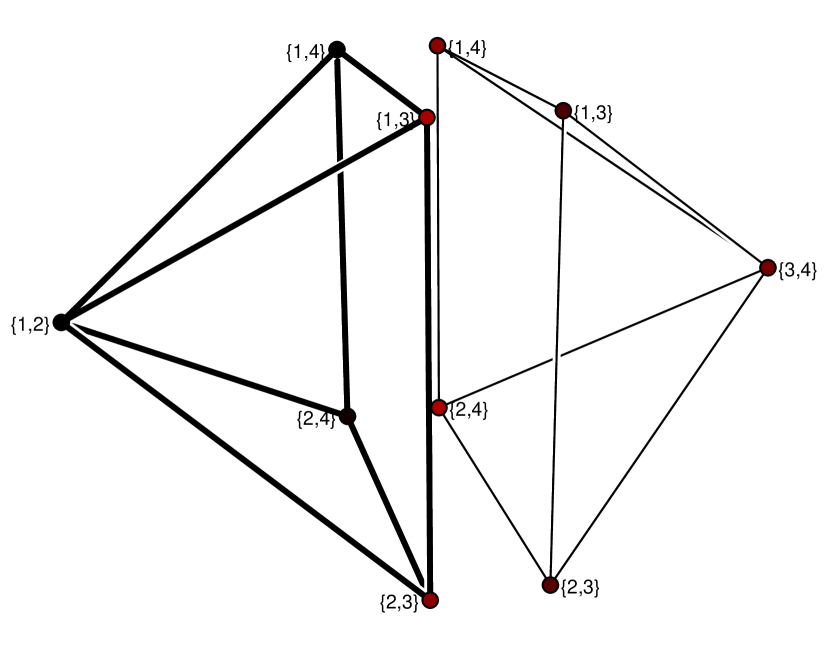
Figure 6. Matroid and matroid subdivision induced by a split as explained in Example 57.

As in the case of the tropical Grassmannian, we can intersect the fan ${{\rm pre-}{\mathscr{G}}_{k,n}}$ with the unit sphere in ${\mathbb{R}}^{\tbinom{n}{k}-n}$ to arrive at a (spherical) polytopal complex ${{\rm pre-}{\mathscr{G}}^{\prime}_{k,n}}$, which we also call the tropical pre-Grassmannian. The following is one of our main results.

Theorem 58.

The split complex ${\rm Split}({\Delta(k,n)})$ is a polytopal subcomplex of the tropical pre-Grassmannian ${{\rm pre-}{\mathscr{G}}^{\prime}_{k,n}}$.

Proof.

By Proposition 26, the split complex is a subcomplex of ${\rm SecFan}^{\prime}({\Delta(k,n)})$. Furthermore, by Lemma 54 each split corresponds to a ray of ${{\rm pre-}{\mathscr{G}}_{k,n}}$. So it remains to show that all maximal cells of ${\Sigma_{{\mathscr{S}}}({\Delta(k,n)})}$ are matroid polytopes whenever ${\mathscr{S}}$ is a compatible system of splits. The proof will proceed by induction on $k$ and $n$. Note that, since ${\Delta(k,n)}\cong{\Delta(n-k,n)}$, it is enough to have as base case $k=2$ and arbitrary $n$, which is given by Proposition 61.

By Theorem 51, we have to show that there do not occur any edges in ${\Sigma_{{\mathscr{S}}}({\Delta(k,n)})}$ that are not edges of ${\Delta(k,n)}$. Since ${\mathscr{S}}$ is compatible no split hyperplanes meet in the interior of ${\Delta(k,n)}$, and so additional edges could only occur in the boundary. By Observation 12, for each split $S\in{\mathscr{S}}$ and each facet $F$ of ${\Delta(k,n)}$ there are two possibilities: Either $H_{S}$ does not meet the interior of $F$, or $H_{S}$ induces a split $S^{\prime}$ on $F$. The restriction of ${\Sigma_{{\mathscr{S}}}({\Delta(k,n)})}$ to $F$ equals the common refinement of all such splits $S^{\prime}$. So, using the induction hypothesis and again Theorem 51, it suffices to prove that the split systems that arise in this fashion are compatible.

So let $S=(A,B,\mu)\in{\mathscr{S}}$. We have to consider to types of facets of ${\Delta(k,n)}$ induced by $x_{i}=0$, $x_{i}=1$, respectively. In the first case, the arising facet $F$ is isomorphic to ${\Delta(k,n-1)}$ and, if $H_{S}$ meets $F$ in the interior, the split $S^{\prime}$ of $F$ equals $(A\setminus\{i\},B;\mu)$ or $(A,B\setminus\{i\};\mu)$. It is now obvious by Proposition 41 that the system of all such $S^{\prime}$ is compatible if ${\mathscr{S}}$ was.

In the second case, the facet $F$ is isomorphic to ${\Delta(k-1,n-1)}$ and $S^{\prime}$ (again if $H_{S}$ meets the interior of $F$ at all) equals $(A\setminus\{i\},B;\mu)$ or $(A,B\setminus\{i\};\mu-1)$. To show that a split system is compatible it suffices to show that any two of its splits are compatible. So let $S=(A,B;\mu)$ and $T=(C,D;\nu)$ be compatible splits for ${\Delta(k,n)}$ such that $H_{S}$ and $H_{T}$ meet the interior of $F$, and $S^{\prime}=(A^{\prime},B^{\prime};\mu^{\prime})$, $T^{\prime}=(C^{\prime},D^{\prime};\nu^{\prime})$, respectively, the corresponding splits of $F$. By the remark after Proposition 41, we can suppose that we are in the first case of Proposition 41, that is, $\#(A\cap C)\leq k-\mu-\nu$. We now have to consider the four cases that $i$ is an element of either $A\cap C$, $A\cap D$, $B\cap C$, or $B\cap D$. In the first case, we have $S^{\prime}=(A\setminus\{i\},B;\mu)$ and $T^{\prime}=(C\setminus\{i\},D,\nu)$. We get $\#(A^{\prime}\cap C^{\prime})=\#(A\cap B)-1\leq k-\mu-\nu-1=(k-1)-\mu^{\prime}-\nu^{\prime}$, so $S^{\prime}$ and $T^{\prime}$ are compatible. The other cases follow similarly, and this completes the proof of the theorem. ∎

Construction 59.

We will now explicitly construct the matroid polytopes that occur in the refinement of two compatible splits. So consider two compatible splits of ${\Delta(k,n)}$ defined by an $(A,B;\mu)$- and a $(C,D;\nu)$-hyperplane. These two hyperplanes divide the space into four (closed) regions. Compatibility implies that the intersection of one of these regions with ${\Delta(k,n)}$ is not full-dimensional, two of the intersections are split matroid polytopes, and the last one is a full-dimensional polytope of which we have to show that it is a matroid polytope. It therefore suffices to show that one of the four intersections is a full-dimensional matroid polytope that is not a split matroid polytope.

By Proposition 41 and the remark following its proof, we can assume without loss of generality that $\#(B\cap D)\leq\mu+\nu-k$. Note first that the equation $\sum_{i\in B}x_{i}=\mu$ also defines the $(A,B;\mu)$-hyperplane from Equation (9), since $x_{A\cup B}=k$ for any point $x\in{\Delta(k,n)}$. We will show that the intersection of ${\Delta(k,n)}$ with the two halfspaces defined by

$$\sum_{i\in B}x_{i}\ \leq\ \mu\qquad\text{and}\qquad\sum_{i\in D}x_{i}\ \leq\ \nu$$

is a full dimensional matroid polytope which is not a split matroid polytope.

To this end, we define a matroid on the ground set $[n]$ together with a realization in ${\mathbb{R}}^{k-1}$ as follows. Pick a pair of (affine) subspaces $U_{B}$ and $U_{D}$ of ${\mathbb{R}}^{k-1}$ such that the following holds: $\dim U_{B}=\mu-1$, $\dim U_{D}=\nu-1$, and $\dim(U_{B}\cap U_{D})=\mu+\nu-k-1$. Note that the latter expression is non-negative as $0\leq\#(B\cap D)\leq\mu+\nu-k-1$. The dimension formula then implies that $\dim(U_{B}+U_{D})=\mu-1+\nu-1-\mu-\nu+k+1=k-1$, that is, $U_{B}+U_{D}={\mathbb{R}}^{k-1}$.

Each element in $[n]$ labels a point in ${\mathbb{R}}^{k-1}$ according to the following restrictions. For each element in the intersection $B\cap D$ we pick a point in $U_{B}\cap U_{D}$ such that the points with labels in $B\cap D$ are in general position within $U_{B}\cap U_{D}$. Since $\#(B\cap D)\leq\mu+\nu-k$ the points with labels in $B\cap D$ are also in general position within $U_{B}$. Therefore, for each element in $B\setminus D=B\cap C$ we can pick a point in $U_{B}\setminus(U_{B}\cap U_{D})$ such that all the points with labels in $B$ are in general position within $U_{B}$. Similarly, we can pick points for the elements of $D\cap A$ in $U_{D}\setminus(U_{B}\cap U_{D})$ such that the points with labels in $D$ are in general position within $U_{D}$. Without loss of generality, we can assume that the points with labels in $B$ and the points with labels in $D$ are in relative general position as subsets of $U_{B}+U_{D}={\mathbb{R}}^{k-1}$.

For the remaining elements in $A\cap C=[n]\setminus(B\cup D)$ we can pick points in ${\mathbb{R}}^{k-1}\setminus(U_{B}\cup U_{D})$ such that the points with labels in $A\cap C$ are in general position and the family of sets of points with labels in $B$, $D$, and $A\cap C$, respectively, is in relative general position. By Lemma 53 the matroid generated by this point set has the desired property.

Example 60.

We continue our Example 42, where $k=3$ and $n=6$, considering the compatible splits $(\{1,2,6\},\{3,4,5\};2)$ and $(\{4,5,6\},\{1,2,3\};2)$. In the notation used in Construction 59 we have $A=\{1,2,6\}$, $B=\{3,4,5\}$, $C=\{4,5,6\}$, $D=\{1,2,3\}$, and $\mu=\nu=2$. Hence $A\cap C=\{6\}$, $A\cap D=\{1,2\}$, $B\cap C=\{4,5\}$, and $B\cap D=\{3\}$. The matroid from Construction 59 is displayed in Figure 7. The non-split matroid polytope constructed in the proof of Theorem 58 has the $f$-vector $(18,72,101,59,14)$.

Figure 7. Non-split matroid constructed from two compatible splits in ${\Delta(3,6)}$ as in Example 60.

For the special case $k=2$ the structure of the tropical Grassmannian and pre-Grassmannian is much simpler. The following proposition follows from [38, Theorem 3.4], in connection with Theorem 49.

Proposition 61.

The tropical Grassmannian ${{\mathscr{G}}^{\prime\prime\prime}_{2,n}}$ equals ${{\rm pre-}{\mathscr{G}}^{\prime}_{2,n}}$, and it is a simplicial complex which is isomorphic to the split complex ${\rm Split}({\Delta(2,n)})$.

Let us revisit the two smallest cases: The tropical Grassmannian ${{\mathscr{G}}^{\prime\prime\prime}_{2,4}}$ consists of three isolated points corresponding to the three splits of the regular octahedron, and ${{\mathscr{G}}^{\prime\prime\prime}_{2,5}}$ is a $1$-dimensional simplicial complex isomorphic to the Petersen graph; see Figure 5.

Proposition 62.

The rays in ${{\rm pre-}{\mathscr{G}}_{k,n}}$ correspond to the coarsest regular matroid subdivisions of ${\Delta(k,n)}$.

Proof.

By definition, a ray in ${{\rm pre-}{\mathscr{G}}_{k,n}}$ defines a regular matroid subdivision which is coarsest among the matroid subdivisions of ${\Delta(k,n)}$. We have to show that this is a coarsest among all subdivisions.

To the contrary, suppose that $\Sigma$ is a coarsest matroid subdivision which can be coarsened to a subdivision $\Sigma^{\prime}$. By construction the $1$-skeleton of $\Sigma^{\prime}$ is contained in the $1$-skeleton of $\Sigma$. From Theorem 51 it follows that $\Sigma^{\prime}$ is matroidal. This is a contradiction to $\Sigma$ being a coarsest matroid subdivision. ∎

Example 63.

In view of Proposition 61, the first example of a tropical Grassmannian that is not covered by the previous results is the case $k=3$ and $n=6$. So we want to describe how the split complex ${\rm Split}({\Delta(3,6)})$ is embedded into ${{\mathscr{G}}^{\prime\prime\prime}_{3,6}}$. We use the notation of [38, Section 5]; see also [37, Section 4.3].

The tropical Grassmannian ${{\mathscr{G}}^{\prime\prime\prime}_{3,6}}$ is a pure $3$-dimensional simplicial complex which is not a flag complex. Its $f$-vector reads $(65,550,1395,1035)$, and its homology is concentrated in the top dimension. The only non-trivial (reduced) homology group (with integral coefficients) is $H_{3}({{\mathscr{G}}^{\prime\prime\prime}_{3,6}};{\mathbb{Z}})={\mathbb{Z}}^{126}$.

The splits with $A=\{1\}\cup A_{1}$, $\mu=1$, and $A=\{1\}\cup A_{3}$, $\mu=2$, are the 15 vertices of type “F”. The splits with $A=\{1\}\cup A_{2}$ and $\mu\in\{1,2\}$ are the 20 vertices of type “E”. Here $A_{m}$ is an $m$-element subset of $\{2,3,\dots,n\}$. The remaining 30 vertices are of type “G”, and they correspond to coarsest subdivisions of ${\Delta(3,6)}$ into three maximal cells. Hence they do not occur in the split complex. See also Billera, Jia, and Reiner [4, Example 7.13].

The 100 edges of type “EE” and the 120 edges of type “EF” are the ones induced by compatibility. Since ${\rm Split}({\Delta(3,6)})$ does not contain any “FF”-edges it is not an induced subcomplex of ${{\mathscr{G}}^{\prime\prime\prime}_{3,6}}$. The matroid shown in Figure 7 arises from an “EE”-edge.

The split complex is $3$-dimensional and not pure; it has the $f$-vector $(35,220,360,30)$. The 30 facets of dimension $3$ are the tetrahedra of type “EEEE”. The remaining 240 facets are “EEF”-triangles.

The integral homology of ${\rm Split}({\Delta(3,6)})$ is concentrated in dimension two, and it is free of degree $144$.

Remark 64.

Example 63 and Proposition 61 show that the split complex is a subcomplex of ${{\mathscr{G}}^{\prime\prime\prime}_{k,n}}$ if $d=2$ or $n\leq 6$. However, this does not hold in general: Consider the weight functions $w,w^{\prime}$ defined in the proof of [38, Theorem 7.1]. It is easily seen from Proposition 41 that $w$ and $w^{\prime}$ are the sum of the weight functions of compatible systems of vertex splits for ${\Delta(3,7)}$. Yet in the proof of [38, Theorem 7.1], it is shown that $w,w^{\prime}\not\in{{\mathscr{G}}^{\prime\prime\prime}_{3,7}}$ for fields with characteristic not equal to $2$ and equal to $2$, respectively.

8. Open Questions and Concluding Remarks

We showed that special split complexes of polytopes (e.g., of the polygons and of the second hypersimplices) already occurred in the literature albeit not under this name. So the following is natural to ask.

Question 65.

What other known simplicial complexes arise as split complexes of polytopes?

The split hyperplanes of a polytope define an affine hyperplane arrangement. For example, the coordinate hyperplane arrangements arises as the split hyperplane arrangement of the cross polytopes; see Example 33.

Question 66.

Which hyperplane arrangements arise as split hyperplane arrangements of some polytope?

Jonsson [21] studies generalized triangulations of polygons; this has a natural generalization to simplicial complexes of split systems such that no $k+1$ splits in such a system are totally incompatible. See also [33, 10].

Question 67.

How do such incompatibility complexes look alike for other polytopes?

All computations with polytopes, matroids, and simplicial complexes were done with polymake [12]. The visualization also used JavaView [34].

We are indebted to Bernd Sturmfels for fruitful discussions. We also thank Hiroshi Hirai and an anonymous referee for several useful comments.

References

- [1] Hans-Jürgen Bandelt and Andreas Dress, Reconstructing the shape of a tree from observed dissimilarity data, Adv. in Appl. Math. 7 (1986), no. 3, 309–343. MR MR858908 (87k:05060)
- [2] by same author, A canonical decomposition theory for metrics on a finite set, Adv. Math. 92 (1992), no. 1, 47–105. MR MR1153934 (93h:54022)
- [3] Louis J. Billera, Susan P. Holmes, and Karen Vogtmann, Geometry of the space of phylogenetic trees, Adv. in Appl. Math. 27 (2001), no. 4, 733–767. MR MR1867931 (2002k:05229)
- [4] Louis J. Billera, Ning Jia, and Victor Reiner, A quasisymmetric function for matroids, 2006, preprint arXiv:math.CO/0606646.
- [5] Ethan D. Bolker, A class of convex bodies, Trans. Amer. Math. Soc. 145 (1969), 323–345. MR MR0256265 (41 #921)
- [6] Peter Buneman, A note on the metric properties of trees, J. Combinatorial Theory Ser. B 17 (1974), 48–50. MR MR0363963 (51 #218)
- [7] Jesús A. De Loera, Jörg Rambau, and Francisco Santos, Triangulations, Springer, to appear.
- [8] Jesús A. De Loera, Bernd Sturmfels, and Rekha R. Thomas, Gröbner bases and triangulations of the second hypersimplex, Combinatorica 15 (1995), no. 3, 409–424. MR MR1357285 (97b:13035)
- [9] Mike Develin and Bernd Sturmfels, Tropical convexity, Doc. Math. 9 (2004), 1–27 (electronic), correction: ibid., pp. 205–206. MR MR2054977 (2005i:52010)
- [10] Andreas Dress, Stefan Grünewald, Jakob Jonsson, and Vincent Moulton, The simplicial complex of compatible line arrangements in the hyperbolic plane - part 1: The structure of , 2007.
- [11] Andreas Dress, Katharina T. Huber, and Vincent Moulton, An exceptional split geometry, Ann. Comb. 4 (2000), no. 1, 1–11. MR MR1763946 (2001h:92005)
- [12] Ewgenij Gawrilow and Michael Joswig, polymake: a framework for analyzing convex polytopes, Polytopes–combinatorics and computation (Oberwolfach, 1997), DMV Sem., vol. 29, Birkhäuser, Basel, 2000, pp. 43–73. MR 2001f:52033
- [13] Israil M. Gel′fand, Mark Goresky, Robert D. MacPherson, and Vera V. Serganova, Combinatorial geometries, convex polyhedra, and Schubert cells, Adv. in Math. 63 (1987), no. 3, 301–316. MR MR877789 (88f:14045)
- [14] Israil M. Gel′fand, Mikhail M. Kapranov, and Andrey V. Zelevinsky, Discriminants, resultants, and multidimensional determinants, Mathematics: Theory & Applications, Birkhäuser Boston Inc., Boston, MA, 1994. MR MR1264417 (95e:14045)
- [15] Sven Herrmann and Michael Joswig, Bounds on the -vectors of tight spans, Contrib. Discrete Math. 2 (2007), no. 2, 161–184 (electronic). MR MR2358269
- [16] Hiroshi Hirai, Characterization of the distance between subtrees of a tree by the associated tight span, Ann. Comb. 10 (2006), no. 1, 111–128. MR MR2233884 (2007f:05058)
- [17] by same author, A geometric study of the split decomposition, Discrete Comput. Geom. 36 (2006), no. 2, 331–361. MR MR2252108 (2007f:52025)
- [18] Peter Huggins, Bernd Sturmfels, Josephine Yu, and Debbie S. Yuster, The hyperdeterminant and triangulations of the 4-cube, Math. Comp. 77 (2008), 1653–1679.
- [19] Daniel H. Huson and David Bryant, Application of phylogenetic networks in evolutionary studies, Mol. Biol. Evol. 23 (2006), no. 2, 254–267.
- [20] J. R. Isbell, Six theorems about injective metric spaces, Comment. Math. Helv. 39 (1964), 65–76. MR MR0182949 (32 #431)
- [21] Jakob Jonsson, Generalized triangulations and diagonal-free subsets of stack polyominoes, J. Combin. Theory Ser. A 112 (2005), no. 1, 117–142. MR MR2167478 (2006d:05011)
- [22] Michael Joswig, Projectivities in simplicial complexes and colorings of simple polytopes, Math. Z. 240 (2002), no. 2, 243–259. MR MR1900311 (2003f:05047)
- [23] Michael Joswig and Katja Kulas, Tropical and ordinary convexity combined, 2008, preprint arXiv:0801.4835.
- [24] Mikhail M. Kapranov, Chow quotients of Grassmannians. I, I. M. Gel′fand Seminar, Adv. Soviet Math., vol. 16, Amer. Math. Soc., Providence, RI, 1993, pp. 29–110. MR MR1237834 (95g:14053)
- [25] Sangwook Kim, Flag enumeration of matroid base polytopes, 2008, unpublished.
- [26] Shungo Koichi, The buneman index via polyhedral split decomposition, 2006, METR 2006-57.
- [27] Jack H. Koolen and Vincent Moulton, A note on the uniqueness of coherent decompositions, Adv. in Appl. Math. 19 (1997), no. 4, 444–449. MR MR1479012 (98j:54050)
- [28] Jack H. Koolen, Vincent Moulton, and Udo Tönges, The coherency index, Discrete Math. 192 (1998), no. 1-3, 205–222, Discrete metric spaces (Villeurbanne, 1996). MR MR1656733 (99g:54027)
- [29] Thomas Lam and Alexander Postnikov, Alcoved Polytopes I, 2005, preprint arXiv:math.CO/0501246.
- [30] Carl W. Lee, Subdivisions and triangulations of polytopes, Handbook of discrete and computational geometry, CRC Press Ser. Discrete Math. Appl., CRC, Boca Raton, FL, 1997, pp. 271–290. MR MR1730170
- [31] Hannah Markwig and Josephine Yu, The space of tropically collinear points is shellable, 2007, preprint arXiv:0711.0944.
- [32] Julian Pfeifle, The secondary polytope of the -cube, Electronic Geometry Models (2000), www.eg-models.de/2000.09.031.
- [33] Vincent Pilaud and Francisco Santos, Multi-triangulations as complexes of star polygons, Discrete Comput. Geom. (to appear), preprint arXiv:0706.3121.
- [34] Konrad Polthier, Klaus Hildebrandt, Eike Preuss, and Ulrich Reitebuch, JavaView, version 3.95, http://www.javaview.de, 2007.
- [35] Alan Robinson and Sarah Whitehouse, The tree representation of , J. Pure Appl. Algebra 111 (1996), no. 1-3, 245–253. MR MR1394355 (97g:55010)
- [36] David E Speyer, Tropical linear spaces, 2004, preprint arXiv:math.CO/0410455.
- [37] by same author, Tropical geometry, Ph.D. thesis, UC Berkeley, 2005.
- [38] David E Speyer and Bernd Sturmfels, The tropical Grassmannian, Adv. Geom. 4 (2004), no. 3, 389–411. MR MR2071813 (2005d:14089)
- [39] Richard P. Stanley, Eulerian partitions of the unit hypercube, Higher Combinatorics (M. Aigner, ed.), D. Reidel, 1977, p. 49.
- [40] Bernd Sturmfels, Gröbner bases and convex polytopes, University Lecture Series, vol. 8, American Mathematical Society, Providence, RI, 1996. MR MR1363949 (97b:13034)
- [41] Henryk Trappmann and Günter M. Ziegler, Shellability of complexes of trees, J. Combin. Theory Ser. A 82 (1998), no. 2, 168–178. MR MR1620865 (99f:05122)
- [42] Karen Vogtmann, Local structure of some -complexes, Proc. Edinburgh Math. Soc. (2) 33 (1990), no. 3, 367–379. MR MR1077791 (92d:57002)
- [43] Neil White (ed.), Theory of matroids, Encyclopedia of Mathematics and its Applications, vol. 26, Cambridge University Press, Cambridge, 1986. MR MR849389 (87k:05054)
- [44] Neil White (ed.), Matroid applications, Encyclopedia of Mathematics and its Applications, vol. 40, Cambridge University Press, Cambridge, 1992. MR MR1165537 (92m:05004)
- [45] Günter M. Ziegler, Lectures on polytopes, Graduate Texts in Mathematics, vol. 152, Springer-Verlag, New York, 1995. MR MR1311028 (96a:52011)