Pulsation-Initiated Mass Loss in Luminous Blue Variables: A Parameter Study

Abstract

Luminous blue variables (LBVs) are characterized by semi-periodic episodes of enhanced mass-loss, or outburst. The cause of these outbursts has thus far been a mystery. One explanation is that they are initiated by $\kappa$-effect pulsations in the atmosphere caused by an increase in luminosity at temperatures near the so-called “iron bump” ($T\sim$ 200,000 K), where the Fe opacity suddenly increases. Due to a lag in the onset of convection, this luminosity can build until it exceeds the Eddington limit locally, seeding pulsations and possibly driving some mass from the star. We present some preliminary results from a parameter study focusing on the conditions necessary to trigger normal S-Dor type (as opposed to extreme $\eta$-Car type) outbursts. We find that as $Y$ increases or $Z$ decreases, the pulsational amplitude decreases and outburst-like behavior, indicated by a large, sudden increase in photospheric velocity, becomes likes likely.

1 Introduction

Luminous blue variables (LBV) represent a short-lived phase of massive star evolution characterized by episodes of intense mass loss, or outburst. There are two main types of outburst behavior. The rare eruptions such as happened with $\eta$-Car and P-Cyg, occur every few decades to centuries. They last as long as a few tens of years and blow off $\geq 1M_{\odot}$ of material in a single episode. The star also experiences an increase in luminosity during this eruption phase.

In contrast, the more normal S-Dor-type episodes occur every few months to few years. They eject $\sim 10^{-4}M_{\odot}$ per event. The LBV does not become more luminous during these episodes. For the purposes of this paper, we will call the more extreme $\eta$-Car-like episodes eruptions and the less extreme S-Dor-like episodes outbursts.

[Vink & de Koter (2002), Vink & de Koter (2002)] determined that the outburst phase results from changes in the dominant ionization states of Fe in the wind which result from changes in the stellar radius and effective temperature, but what causes the changes in the radius and temperature is not clear. In this paper we explore the hypothesis that it is due to seeding from $\kappa$-effect pulsations arising from a large increase in luminosity due to the increase in Fe opacity from the so-called “hot iron bump” at temperatures near 200,000 K. We will also discuss the possiblity that a super-Eddington luminosity in regions of the star near these iron bump temperatures could directly drive mass from the star.

2 Models

We start with massive main sequence models in the mass range $50M_{\odot}\leq M_{*}\leq 80M_{\odot}$. We evolve the stars using the Iben evolution code [Iben (1965), (Iben 1965)]. Important additions to the code are the Swenson SRIFF analytical EOS, OPAL opacities using the Grevesse and Noels 93 mixture (as used in [Iglesias & Rogers (1996), Iglesias & Rogers (1996)]), and the empirical mass-loss prescription of [Nieuwenhuijzen & de Jager (1990), Nieuwenhuijzen & de Jager (1990)]. We vary the mass-loss rate to allow different surface abundances at the end of the evolution. More details of this and the other codes used in this analysis are found in [Guzik et al.(2005), Guzik, Watson, & Cox (2005)].

Once we have a model with properties similar to an LBV star, we run the model through a pulsation analysis code. This code determines the first three harmonics of the $\kappa$-effect pulsations. The most unstable mode – that is, the one with the largest growth rate, as determined by the fractional energy gain per period – is then chosen for further analysis. The modes chosen for this analysis are shown in Table 1. We analyze this unstable mode using the 1D Lagrangian hydrodynamics code Dynstar [Cox & Ostlie (1993), (Cox & Ostlie 1993)]. This code includes the time-dependent convection treatment formulated by [cox90, Ostlie (1990)] and described below.

Table 1: Properties of analyzed modes

Y	Z	Mode1	Fractional Energy
			Gain / Period
29	0.01	1H	1.11
29	0.02	1H	2.07
49	0.01	1H	0.552
49	0.02	1H	2.22

The models have log $L/L_{\odot}\approx 6.1$ and $T_{eff}=1.6\times 10^{4}$ K. We vary the metallicity $Z$ and the helium abundance $Y$. Since the pulsations are driven by iron opacity, they are $Z$-dependent, with lower $Z$ resulting in smaller amplitudes. As $Y$ is increased, the star effectively becomes older and closer to the stable Wolf-Rayet phase, also resultin in smaller pulsation amplitudes.

3 Time-Dependent Convection

Our time-dependent convection model is described in detail in [Ostlie (1990), Ostlie (1990)]. Here are the main highlights.

The time-dependent convection model is built upon standard mixing length theory [bohmyy, Cox & Giuli(1968), (Bohm ??; Cox & Giuli 1968)]. In the standard theory the convective luminosity is

$$L_{c}=4\pi r^{2}\frac{4T\rho C_{P}}{g\ell Q}v_{c}^{0\;3},$$ (1)

where $r,T,C_{P},\rho,$ and $g$ are the local radius, temperature, specific heat, density, and gravitational acceleration, respectively. The mixing length $\ell$ is assumed to be equal to the pressure scale height. The parameter $Q$ defined

$$Q\equiv-\frac{\partial\log\rho}{\partial\log T}|_{P}.$$ (2)

$Q=1$ for an ideal gas with a constant mean molecular weight. The convective eddy velocity in the static case is

$$v_{c}^{0}=\frac{1}{4}\sqrt{\frac{gQ\ell^{2}}{2H_{P}}f},$$ (3)

where $H_{P}$ is the pressure scale height,

$$f\equiv[\sqrt{1+4A^{2}(\Delta-\Delta_{ad})}-1]/A,$$ (4)

$$\Delta\equiv\frac{d\log T}{d\log P},$$ (5)

$$A\equiv\frac{Q^{1/2}\>C_{P}\kappa g\rho^{5/2}\>\ell^{2}}{12\sqrt{2}acP^{1/2}\>T^{3}},$$ (6)

$\Delta-\Delta_{ad}$ is the superadiabatic gradient, and $\kappa$ is the local opacity.

The static case, however, does not account for the effect of convective lag due to the inertia of the material. This lag is included in our model using a quadratic Lagrange interpolation polynomial of $v_{c}$ over the current and previous two time steps.

For zone $i$ and time step $n$ the time-dependent value of $v_{c}$ is

$$v_{c,\>i}^{n} \equiv \frac{(t^{\prime}-t_{n-1})(t^{\prime}-t_{n-2})}{(t_{n}-t_{n-1})(t_{n}-t_{n-2})}v_{c,\>i}^{0}+\frac{(t^{\prime}-t_{n})(t^{\prime}-t_{n-2})}{(t_{n-1}-t_{n})(t_{n-1}-t_{n-2})}v_{c,\;i}^{n-1}$$

$$+ \frac{(t^{\prime}-t_{n})(t^{\prime}-t_{n-1})}{(t_{n-2}-t_{n})(t_{n-2}-t_{n-1})}v_{c,\>i}^{n-2},$$

where $v_{c\;i}^{0}$ is the value determined from equation 3,

$$t^{\prime}\equiv t_{n-1}+\tau(t_{n}-t_{n-1})$$ (8)

and

$$\tau\equiv\frac{v_{c\;i}^{n}(t_{n}-t_{n-1})}{\ell}l_{fac}.$$ (9)

The lag factor $l_{fac}\equiv 1$ in our models.

4 Results

Figure 1 shows how the photospheric velocity $v_{phot}$ is affected by changing the metallicity. The figure shows the photospheric velocity as a function of time for a model at solar metallicity (defined here as $Z=0.02$) and at half-solar, or LMC-like $Z$. Both models exhibit “outburst”-like behavior, in that extreme super-Eddington zones deep in the star near 200,000 K (see Figure 2) result in a large, sudden increase in the surface velocity. As expected the model with the larger metallicity experienced a larger velocity amplitude.

The $Z=0.01$ model with $Y$ increased to 0.49 is shown in Figure 3. In contrast to the “outburst” models, this model settles into steady pulsations, and Figure 4 shows that this model only becomes super-Eddington by a few percent. Thus the star seems able to recover and settle into steady, albeit very large amplitude ($v_{phot}=100$ km s${}^{-}1$) pulsations.

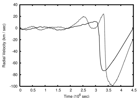
Figure 1: Photospheric velocity as a function of time. Solid line is $Z$ = 0.02, dashed line is $Z$ = 0.01. Negative velocity is outward.

Figure 2: Radiative luminosity at T $\sim$ 210,000 K relative to the Eddington luminosity.

Figure 3: Photospheric velocity as a function of time for the case $Y=0.49,Z=0.01$.

Figure 4: Radiative luminosity at $T\sim$ 210,000 K relative to Eddington for $Y=0.49,Z=0.01$.

5 Conclusions and Future Work

We have preliminary results from a study on $\kappa$-effect pulsations in LBV stars, with possible implications for S-Dor-like mass loss. We have found that regions in the star near $T\sim$ 200,000 K experience large super-Eddington luminosities due to the increase of radiation from iron bump opacities. We have found that this can cause large amplitude pulsations at the surface. At lower $Y$ and higher $Z$, a large sudden increase in radial velocity is seen at the surface. Whether the pulsations or the sudden velocity increases evolve into S-Dor-like outbursts is not clear.

The results presented here are still very preliminary. Much more work is needed to confirm our results. Not the least of which is a zoning study. We have used 60-zone models to improve the throughput, but it is not clear that this is sufficient. Runs at 120 zones and higher should be run in order to confirm that the results are robust.

In addition it is not clear that our “outbursts” result in much, if any mass loss directly. As Owocki, et al. showed in these proceedings, the most likely scenario for mass loss in a super-Eddington atmosphere is one in which the material separates into clumps with the clumps essentially stationary and some small amount of material driven above the escape speed between these clumps. As we have only a 1D analysis thus far, it is impossible for us to determine what the clump size distribution would be.

This is the beginning of a more formal parameter study on the nature of these pulsations and their connections, if any, to S-Dor behavior. In addition to more coverage of the parameter space, we eventually plan to extend the hydrodynamic analysis to 2D to determine whether the super-Eddington nature of the pulsations leads to enhanced mass loss through pores in the stellar atmosphere.

LangerHow many pulsation cycles does it take to lose the pulsating layer in a stationary wind, assuming standard radiation-driven wind mass-loss rates?

OniferThe pulsation cycle for the model I showed was about 1 month, and the Fe bump region is $\sim 10^{-3}M_{\odot}$ below the surface, so it would take about 100 years or $\sim$ 1000 pulsation cycles to strip away the layer.

HumphreysThanks for making the distinction between the normal or classical LBVs like S Dor & AG Car and the $\eta$ Car-like giant eruptions. $\eta$ Car & its rare relatives actually increase their luminosity during their giant eruptions. The classical LBVs maintain constant luminosity during their optically thick wind stage. Owocki was talking about $\eta$-Car-like eruptions. It may only be a difference of degree, and the mechanism may be the same, but what we observe is very different. It is important to make the distinction.

OniferThank you, this is a very good point.

HirschiIf pulsations are driven by iron opacity, pulsations would be strongly metallicity dependent. Are there other sources of opacity at very low metallicities to drive pulsations.

OniferI’m not aware of any sources of opacity at similar temperatures that could take over for iron at low metallicity.