Blind Date: Using proper motions to determine the ages of historical images

Abstract

Astrometric calibration is based on patterns of cataloged stars and therefore effectively assumes a particular epoch, which can be substantially incorrect for historical images. With the known proper motions of stars we can “run back the clock” to an approximation of the night sky in any given year, and in principle the year that best fits stellar patterns in any given image is an estimate of the year in which that image was taken. In this paper we use 47 scanned photographic images of M44 spanning years 1910–1975 to demonstrate this technique. We use only the pixel information in the images; we use no prior information or meta-data about image pointing, scale, orientation, or date. Blind Date returns date meta-data for the input images. It also improves the astrometric calibration of the image because the final astrometric calibration is performed at the appropriate epoch. The accuracy and reliability of Blind Date are functions of image size, pointing, angular resolution, and depth; performance is related to the sum of proper-motion signal-to-noise ratios for catalog stars measured in the input image. All of the science-quality images and $85$ percent of the low-quality images in our sample of photographic plate images of M44 have their dates reliably determined to within a decade, many to within months.

1 Introduction

Astronomy needs well calibrated data to make precise measurements, but also wants to make use of large data sources that are poorly calibrated. Unreliable data sets such as historical archives, amateurs collections, and engineering data contain important information, especially in the time domain. Astronomy needs methods by which data of unknown provenance, quality, and calibration can be vetted, calibrated, and made reliably useable by the community.

There is an enormous amount of information about proper motions, stellar and AGN variability, transients, and Solar System bodies in historical plate archives and the collections of good amateur astronomers. The Harvard College Observatory Astronomical Plate Stacks alone contain enough photographic exposures to cover the entire sky 500 times over, and span many decades with good coverage and imaging depth. However, in many cases, it is challenging to use those images quantitatively. Often the details of observing date, telescope pointing, bandpass, and exposure time are lost because the logs have been lost, because the information was written incorrectly or illegibly, or because it is difficult or expensive to associate each image with the appropriate record in the log.

The astronomical world is moving towards the development of a Virtual Observatory, in which a heterogeneous set of data providers communicate with researchers and the public through open data-sharing protocols. These protocols can be easily spoofed—intentionally and unintentionally—and permit the dissemination of badly calibrated, erroneous, or untrustworthy data. Indeed, the lack of a “trust” model may compromise the VO’s goals of making it easy for astronomers to discover and use wide varieties of input data; without trust, all the time that saved in searching and using has to be spent in verification and tracking of provenance.

Amateur astronomers and educators at college/planetarium observatories are, in many cases, well equipped and can take science-quality observations, especially for time-domain science. In addition, most of these astronomers are interested in contributing to research astronomy. However, it is challenging at present for these potential data providers to provide their data to the community in a form that is trivially useable by the research community. These observers need automated systems to calibrate their data and hardware and to package the data and meta-data in standards-compliant forms. Even professional observatories often produce data with incorrect or standards-violating meta-data because of telescope faults, software bugs, or the youth of most standards and conventions for digital data formats.

We have begun a large project (Astrometry.net) to vet, restore, determine, and package in standards-compliant form the calibration meta-data for astronomical images for which such information is lost, damaged, or unreliable (Lang et al, 2008). Our system can astrometrically calibrate an image (that is, determine the world coordinate system) using the information in the image pixels alone. It starts by identifying asterisms that determine astrometric calibration. Once the astrometry is correct, the sources in the image can be identified with catalogs and other calibration meta-data can be inferred through quantitative image analysis. In the process of testing and running this calibration system, we have indeed confirmed that many historical and amateur images—and even some scientific images from modern professional facilities—have missing or incorrect astrometric meta-data; automated calibration, as a vetting step at the very least, is essential for all data sources.

For the same reason that the time domain is interesting, it can also be used to calibrate the date at which an image was taken. Stars are moving and varying, so the particular configuration and relative brightnesses of the stars in an image provide, in principle, a measure of the time at which the image was taken. Here we show that stellar motions catalogued at the present day can be used to age-date plates from a plate archive to within a few years, even for very old plates. This new capability takes the Astrometry.net project a small step closer to being a comprehensive image meta-data vetting and automated calibration system.

2 Input data

The larger goal of our project is to add calibration meta-data to data of unknown provenance. For this reason, the system begins truly “blind” in the sense that we ignore all meta-data associated with each input image, and start with only the image pixels themselves. We calibrate the images using the Astrometry.net astrometric system; this calibration provides output that is taken as input data for the Blind Date analysis.

For each automatically detected star $i$ in the image, there is a centroid $(x_{i},y_{i})$ in the input image measured in pixels. For each source, this centroid is the location of the maximum of a second-order polynomial (generalized parabolic) surface fit to the area immediately surrounding the center of the image star. The fit also provides uncertainties $(\sigma_{x{i}},\sigma_{y{i}})$ in these centroids. For unsaturated stars these are taken (arbitrarily) to be one pixel, and for saturated stars (which are common in the digitized plate data) these are taken to be one-third of the radius of the saturated region. These are over-estimates, since the stars are detected at good signal-to-noise, but this is conservative; furthermore, in the case of saturated stars, it is possible for the saturated “disk” to be non-concentric with the true centroid.

The system also provides a rough world coordinate system (WCS) for the image; that is, first guesses at two functions: $WCS_{xy\rightarrow\mathrm{RD}}(x,y)$, which transforms points from the image plane in pixels into celestial coordinates in angular units, and $WCS_{\mathrm{RD}\rightarrow xy}(\mathrm{RA},\mathrm{Dec})$, the inverse. A derived quantity from these functions is the pixel scale $\theta_{\mathrm{pix}}$, measured in angle per pixel, which we will use below. Strictly $\theta_{\mathrm{pix}}$ is a function of position in the image, but in typical science images it does not vary substantially.

The WCS effectively identifies the sources from the USNO-B Catalog (Monet et al, 2003) that are in or likely to be in the image. For each catalog “star” $j$ (the USNO-B Catalog contains both stars and compact galaxies) inside the image, the catalog contains a J2000 celestial position $(\mathrm{RA}_{j},\mathrm{Dec}_{j})$ on the celestial sphere (extrapolated to epoch $2000.0$) measured in angular units, an uncertainty $(\sigma_{\mathrm{RA}{j}},\sigma_{\mathrm{Dec}{j}})$ in that position, a proper motion $(\mu_{\mathrm{RA}{j}},\mu_{\mathrm{Dec}{j}})$ measured in angle per time, and an uncertainty $(\sigma_{\mu\mathrm{RA}{j}},\sigma_{\mu\mathrm{Dec}{j}})$ in that proper motion.

The USNO-B Catalog uncertainties required some processing and adjustment. For the sake of clarity and simplicity, we make as few assumptions as possible in transforming the uncertainties. Our approach here is not intended to be definitive. Many of these entries in the catalog have values of zero for the uncertainty of position or proper motion. In the case of zero-valued uncertainty in position, we assume that the uncertainty is below the precision of $0.002\,\mathrm{arcsec}$ at which the catalog was reported. We therefore set all zero-valued position uncertainties to one-half of the precision ($0.001\,\mathrm{arcsec}$). For entries with zero-valued uncertainty in proper motion, there is more we need to consider; a nonzero-valued proper motion paired with a zero-valued uncertainty indicates that the uncertainty is below the precision of the catalog, and therefore should be set to half of the precision. A zero-valued proper motion paired with a zero-valued uncertainty indicates that the proper motion of the entry could not be measured accurately (Dave Monet, private communication). We therefore set the uncertainty in the proper motion for such entries to three times the median value of nonzero proper motion uncertainties. This captures the idea that, generally speaking, we are significantly more uncertain about the proper motion of such entries than we are most other entries. A more principled approach could certainly be attempted but we found that this worked well enough for our purposes.

Much work has already been done by the Astrometry.net team to identify spurious sources in the USNO-B Catalog that appear to have been created by diffraction spikes and reflection halos (Barron et al, 2008). For the purposes of this project, we ignore the entries in the catalog which have been flagged as spurious. Testing has shown that ignoring these sources generally improves the accuracy of our results.

Using a technique that will be described in a future paper from the Astrometry.net team, we are able to estimate the bandpass of each image being processed, in that we determine which bandpass of the USNO-B Catalog most closely predicts the brightness ordering of the stars in the image. Though this technique is still in an experimental stage, its results are not very controversial; all of Harvard’s images of M44 appear to best match the blue bands ($O$ and $J$ emulsions) of the USNO-B Catalog. This finding is reinforced through experimentation with manually setting each image’s band: On average, Blind Date performs better on these images using the $J$ emulsion of the Catalog than on any other band.

Assuming that we have estimated the bandpass correctly, the $N$ stars in the image should correspond—roughly—to the $N$ brightest catalog stars that lie within the area of the image. For that reason, we use only the $N$ brightest catalog stars in what follows.

3 Method

We use the USNO-B Catalog positions and proper motions to “wind” the $N$ catalog stars backwards and forward through time along the celestial sphere. Once the catalog has been adjusted, we can use the image WCS to project the catalog entries onto the image plane, making a synthetic catalog for that image at that time, in image coordinates. We then attempt to fit the image stars to that synthetic image of the moved catalog stars. We choose a freedom with which the image star positions are allowed to warp to fit the catalog star positions, and a scalar objective function that is minimized when the positions are “best” warped. We warp the input image to the catalog “wound” to different times, and use the best-fit values of the objective function to determine the year at which the image was taken.

3.1 Winding back the catalog

We estimate the celestial coordinates of catalog star $j$ at the arbitrary date $t$, and then project them onto the image plane

$$\displaystyle\left(u_{j},v_{j}\right) = WCS_{\mathrm{RD}\rightarrow xy}\left(\mathrm{RA}_{j}-\hat{\mu}_{\mathrm{RA}{j}}[t-(2000.0\,\mathrm{yr})],\mathrm{Dec}_{j}-\mu_{\mathrm{Dec}{j}}[t-(2000.0\,\mathrm{yr})]\right)\quad,$$ (1)

where we have adjusted the $\mu_{\mathrm{RA}{j}}$ proper motion vector components and their associated uncertainties into coordinate derivatives $\hat{\mu}_{\mathrm{RA}{j}}$ by

$$\displaystyle\hat{\mu}_{\mathrm{RA}{j}} = \mathrm{cos}(\mathrm{Dec}_{j})\,\mu_{\mathrm{RA}{j}}$$

$$\hat{\sigma}_{\mu\mathrm{RA}{j}} = \mathrm{cos}(\mathrm{Dec}_{j})\,\sigma_{\mu\mathrm{RA}{j}}\quad.$$ (2)

We estimate the uncertainty of the location of catalog star $j$ at year $t$ on the image plane with

$$\displaystyle\sigma_{u{j}} = \frac{1}{\theta_{\mathrm{pix}}}\,\sqrt{\sigma_{\mathrm{RA}{j}}^{2}+(\max\left(|t-t_{\mathrm{early}}|,|t-t_{\mathrm{late}}|\right)\,\hat{\sigma}_{\mu\mathrm{RA}{j}})^{2}}$$

$$\sigma_{v{j}} = \frac{1}{\theta_{\mathrm{pix}}}\sqrt{\sigma_{\mathrm{Dec}{j}}^{2}+(\max\left(|t-t_{\mathrm{early}}|,|t-t_{\mathrm{late}}|\right)\,\sigma_{\mu\mathrm{Dec}{j}})^{2}}$$ (3)

where $t_{\mathrm{early}}$ and $t_{\mathrm{late}}$ are the dates at which the USNO-B Catalog source imagery were taken, which in this patch of the sky are 1955.0 and 1990.0, respectively. All positions in the Catalog, however, were extrapolated to the year $2000.0$ (epoch and equinox). This means that though we are given each catalog star’s location at the year $2000.0$, we know that each star’s measured location is, in general, more accurate between the two epochs in which the images were taken, and less accurate at years further from that range. This means that when “winding” locations through time, we look at the difference between $t$ and the year $2000.0$; when “winding” uncertainties through time, we look at the maximum distance between $t$ and both $t_{\mathrm{early}}$ and $t_{\mathrm{late}}$. This is equivalent to using $(t_{\mathrm{early}}+t_{\mathrm{late}})/2$ as our reference year, and assuming a non-zero uncertainty on the measurement of each star’s proper motion at that reference year.

Note that in our notation for $(u_{j},v_{j})$ and $(\sigma_{u{j}},\sigma_{v{j}})$, we do not reference $t$. This is because once the catalog has been wound through time and projected onto the image plane, we consider time to be fixed. Note that in Sections 3.2 and 3.3, time will remain fixed, and therefore $t$ is not mentioned in any of the notation except for in $\chi^{2}(t)$.

3.2 Objective function

Determination of the image coordinate system and date involves finding parameters—astrometric parameters and the date—that optimize an objective function. The choice of this objective is therefore the fundamental scientific choice in the project.

We seek an objective function that has the following properties, listed in rough order of priority: The function must decrease as image-coordinate distances between catalog and image stars decrease. The function must be insensitive to anomalous outliers, and more sensitive to well-measured stars than to poorly-measured stars. The function must be some approximation to a likelihood or have some equivalent justification so that changes in the function with respect to parameters can be interpreted in terms of uncertainties in those parameters. The function ought to be differentiable and second-differentiable with respect to all fit parameters (in particular time and astrometric calibration). The function should be easily optimized. We have identified an objective function that has all of these properties; it is so similar to the least-square function that we call it a “modified chi-squared” and denote it “$\chi^{2}$”.

For all $i=1:N$ and $j=1:N$ we compute $d_{ij}$, the Euclidian distance between image star $i$ and catalog stars $j$ in the image plane.

$$d_{ij}=\sqrt{\left(u_{j}-x_{i}\right)^{2}+\left(v_{j}-y_{i}\right)^{2}}$$ (4)

We also estimate the uncertainty $\bar{\sigma}_{ij}$ of each pair’s distance measurement, using the previously defined values for $(\sigma_{x{i}},\sigma_{y{i}})$ and $(\sigma_{u{j}},\sigma_{v{j}})$. We calculate the combined uncertainty for the pair in $x$ and $y$ at time $t$, and then simply take the mean as an estimation of the uncertainty of that pair:

$$\bar{\sigma}_{ij}=\frac{1}{2}\,\left(\sqrt{\sigma_{x{i}}^{2}+\sigma_{u{j}}^{2}}+\sqrt{\sigma_{y{i}}^{2}+\sigma_{v{j}}^{2}}\right)$$ (5)

We define a weighting function for each pair that returns a value between 0 and 1 based on the ratio of the distance of a pair to the uncertainty of that pair:

$$W(d,\bar{\sigma})=\frac{1}{1+\left(\frac{d}{\bar{\sigma}}\right)^{2}}$$ (6)

(see also Figure 1). This function has the property that outliers are down-weighed in a smooth manner; it causes the influence of a image–catalog pair to smoothly drop to zero at large displacement. This permits us to avoid the discontinuous optimization problem of sigma clipping, which is the standard “robust estimation” technique in common use in astronomy applications. The weighting function has a number of properties which make it well-suited to our purpose:

$$\displaystyle W(0,\bar{\sigma}) = 1$$ (7)

$$\left.\frac{\mathrm{d}W}{\mathrm{d}d}(d,\bar{\sigma})\right|_{d=0} = 0$$ (8)

$$\lim_{(d/\bar{\sigma})\rightarrow\infty}W(d,\bar{\sigma})\left(\frac{d}{\bar{\sigma}}\right)^{2} = 1$$ (9)

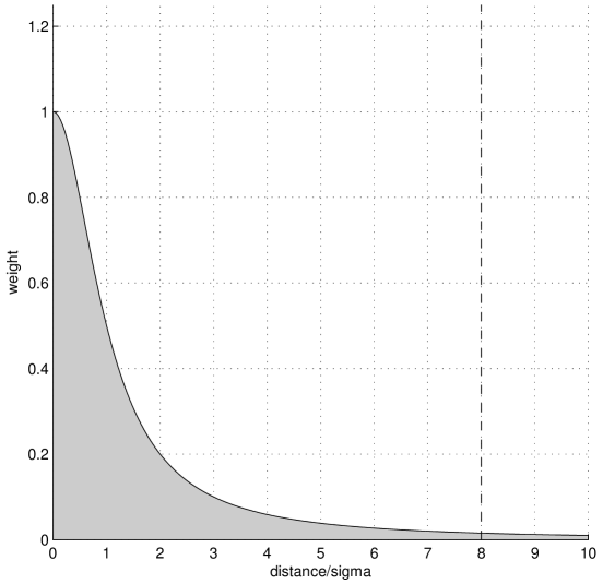
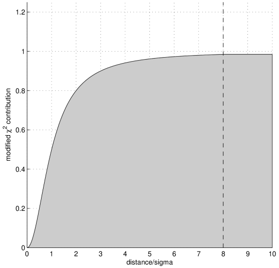
Figure 1: On the left, the weighting function versus a pair’s ratio of distance to uncertainty. On the right, the corresponding weighted contribution of a pair to the modified chi-squared. The dotted line indicates the point at which we assume that the weighted contribution stops changing.

We use this weighting function to assign a weight $w_{ij}$ to all pairs as follows:

$$w_{ij}=W\left(d_{ij},\bar{\sigma}_{ij}\right)$$ (10)

Our final objective function is:

$$\chi^{2}(t)=\sum_{ij}w_{ij}\,\left(\frac{d_{ij}}{\bar{\sigma}_{ij}}\right)^{2}$$ (11)

where the sum is over all possible image–catalog pairs.

For “good” (small-separation) image–catalog pairs, the weight function is near unity (equation 7) and has near-zero derivatives (equation 8), so small changes in separation do not enter strongly into derivatives of the objective function. For “bad” (large-separation) image–catalog pairs, the pair’s contribution to $\chi^{2}(t)$ is nearly constant (equation 9). This makes optimization and interpretation of our objective function very like optimization and interpretation of a chi-squared fitting system. This weighted chi-squared objective function could also be interpreted as a Geman-McLure error function, In this framework, optimizing the objective function is equivalent to robust M-estimation (Hampel et al, 1986).

In constructing the modified chi-squared, we use—in principle—all image–catalog pairs, irrespective of their separation in image coordinates. The fact that the contribution of a pair to the objective function quickly converges to $1$ as the pair becomes highly separated allows us—in practice—to ignore all highly separated pairs. We therefore choose to approximate the contributions of all pairs where $d>8\,\bar{\sigma}$ as $W(8\,\bar{\sigma},\bar{\sigma})\left(\frac{8\bar{\sigma}}{\bar{\sigma}}\right)^{2}$, which is $64/65$. This dramatically speeds up our computation.

3.3 Fitting the image

At this point, we have our image stars on the image plane, our catalog stars (wound to the time of interest) projected onto the image plane, and an objective function that we wish to minimize. We need to find the transformation that we can apply to the image that minimizes the objective function, which we take to be the transformation that best “fits” the image to the catalog.

Testing has suggested that the initial location of the image returned by the Astrometry.net solver is close enough to the optimal location that locally minimizing the objective function is sufficient for finding the global minimum, and that we generally do not run the risk of falling into a false local minimum. Therefore, we only present our method for locally minimizing the optimal function through iteratively reweighted least-squares (IRLS). We experimented with techniques such as RANSAC to fit images to the catalog in the face of extreme noise, but no technique was more effective and robust than our IRLS method.

Let us first construct a solution to a simplified version of this problem, in which we know which correspondences are true: We assume that image point $i$ corresponds to catalog point $i$ for all $i\in\{1,2,...,N\}$. Assuming that we are interested in solving for an affine transformation (first-order linear transformation plus shift), this means that we need to find the transformation matrix that best satisfies the following equations:

$$\underset{i\in\{1,2,...,N\}}{\forall}\,\left[\begin{array}[]{ccc}m_{x}&m_{y}&t_{x}\\ n_{x}&n_{y}&t_{y}\end{array}\right]\left[\begin{array}[]{c}x_{i}\\ y_{i}\\ 1\end{array}\right]=\left[\begin{array}[]{c}u_{i}\\ v_{i}\end{array}\right]$$ (12)

This can be generalized straightforwardly for higher order transformations.

The transformation that best satisfies these equations can be found using a standard least-squares solver. We can then use this transformation to warp all of the image points onto the catalog points (and vice-versa), thus solving our simplified problem.

Of course, since we do not know which image stars correspond to which catalog stars, we must include equations for all image–catalog pairs. We are not interested in the solution to this problem, as it would describe a transformation from every image star to every catalog star. To specify a transformation that satisfies likely image–catalog correspondences, we must use our weighting function to make soft assignments regarding correspondences. We therefore use the following equations:

$$\underset{i\in\{1,2,...,N\}}{\forall}\,\,\,\underset{j\in\{1,2,...,N\}}{\forall}\,\left[\begin{array}[]{cc}\frac{\sqrt{w_{ij}}}{\bar{\sigma}_{ij}}&0\\ 0&\frac{\sqrt{w_{ij}}}{\bar{\sigma}_{ij}}\end{array}\right]\left[\begin{array}[]{ccc}m_{x}&m_{y}&t_{x}\\ n_{x}&n_{y}&t_{y}\end{array}\right]\left[\begin{array}[]{c}x_{i}\\ y_{i}\\ 1\end{array}\right]=\left[\begin{array}[]{cc}\frac{\sqrt{w_{ij}}}{\bar{\sigma}_{ij}}&0\\ 0&\frac{\sqrt{w_{ij}}}{\bar{\sigma}_{ij}}\end{array}\right]\left[\begin{array}[]{c}u_{j}\\ v_{j}\end{array}\right]$$ (13)

We begin our solution by constructing a linear system which contains all of the previously described (unweighted) equations.

$$\left[\begin{array}[]{cccccc}x_{1}&y_{1}&1&0&0&0\\ 0&0&0&x_{1}&y_{1}&1\\ x_{1}&y_{1}&1&0&0&0\\ 0&0&0&x_{1}&y_{1}&1\\ &&\ldots\\ x_{N}&y_{N}&1&0&0&0\\ 0&0&0&x_{N}&y_{N}&1\\ x_{N}&y_{N}&1&0&0&0\\ 0&0&0&x_{N}&y_{N}&1\end{array}\right]\left[\begin{array}[]{c}m_{x}\\ m_{y}\\ t_{x}\\ n_{x}\\ n_{y}\\ t_{y}\end{array}\right]=\left[\begin{array}[]{c}u_{1}\\ v_{1}\\ u_{2}\\ v_{2}\\ \ldots\\ u_{N-1}\\ v_{N-1}\\ u_{N}\\ v_{N}\end{array}\right]$$ (14)

We can write this matrix equation as:

$$\mathbf{Ax}=\mathbf{b}$$ (15)

To introduce the weight values described in the equations, we construct our weight matrix $\mathbf{W}$, as follows:

$$\mathbf{W}=\mathrm{diag}\left(\begin{array}[]{ccccccccc}\frac{\sqrt{w_{1,1}}}{\bar{\sigma}_{1,1}},\frac{\sqrt{w_{1,1}}}{\bar{\sigma}_{1,1}},\frac{\sqrt{w_{1,2}}}{\bar{\sigma}_{1,2}},\frac{\sqrt{w_{1,2}}}{\bar{\sigma}_{1,2}},\ldots,\frac{\sqrt{w_{N,N}}}{\bar{\sigma}_{N,N}},\frac{\sqrt{w_{N,N}}}{\bar{\sigma}_{N,N}}\end{array}\right)$$ (16)

Our final matrix equation can then be written as:

$$\mathbf{WAx}=\mathbf{Wb}$$ (17)

We then find $\mathbf{x}$ such that the squared residuals, $\mathbf{(WAx-Wb)^{T}(WAx-Wb)}$, are minimized. By construction, $\mathbf{x}$ describes the transformation that best satisfies all of the equations we previously constructed, and can be found using a standard least-squares solver.

Using the transformation defined by $\mathbf{x}$ we can calculate the coordinates of our warped image points.

$$\displaystyle{x_{i}}^{\prime} = m_{x}x_{i}+m_{y}y_{i}+t_{x}$$

$${y_{i}}^{\prime} = n_{x}x_{i}+n_{y}y_{i}+t_{y}$$ (18)

Unlike the simplified version of this problem, the warp found after one iteration is not our final solution. As we warp the image, the distances and weights between the image and catalog points change, and so our objective function is no longer minimized. The solution is to repeatedly recalculate our $d_{ij}$ and $w_{ij}$ values and our weighted least squares transformation. We perform this iteratively reweighted least-squares operation until the resulting transformations stop changing, which by construction is also when our objective function stops changing. The solution which we converge upon is returned as the best fit of the image onto the catalog.

The IRLS method minimizes the objective function, as it was constructed such that the objective function is equal to the sum of the squares of the weighted residuals of the matrix equation.

$$\displaystyle\mathbf{(WAx-Wb)^{T}(WAx-Wb)} = \mathbf{(W(Ax-b))^{T}(W(Ax-b))}$$ (19)

$$= \sum_{ij}\left(\frac{\sqrt{w_{ij}}}{\bar{\sigma}_{ij}}\left(u_{j}-{x_{i}}^{\prime}\right)\right)^{2}+\left(\frac{\sqrt{w_{ij}}}{\bar{\sigma}_{ij}}\left(v_{j}-{y_{i}}^{\prime}\right)\right)^{2}$$

$$= \sum_{ij}\left(\frac{\sqrt{w_{ij}}}{\bar{\sigma}_{ij}}{d_{ij}}^{\prime}\right)^{2}$$

$$= \sum_{ij}w_{ij}\left(\frac{{{d_{ij}}^{\prime}}}{\bar{\sigma}_{ij}}\right)^{2}$$

$$\approx \chi^{2}(t)$$

We say that the residuals only approximate the optimal function because we use the weights of the previous transformed image ($w_{ij}$) and the distances of the next warped transformed image (${d_{ij}}^{\prime}$). Though this may seem strange, once the IRLS has converged on a solution and the optimal function has stopped changing, the distances in one iteration are effectively equal to the distances in the following iteration.

For numerical stability we always use the initial coordinates when constructing our transformation, and only return the final warped image coordinates. The intermediate warped image coordinates are only used for calculating distances and weights. This means that our final image coordinates have only been subjected to one transformation, as opposed to many small transformations.

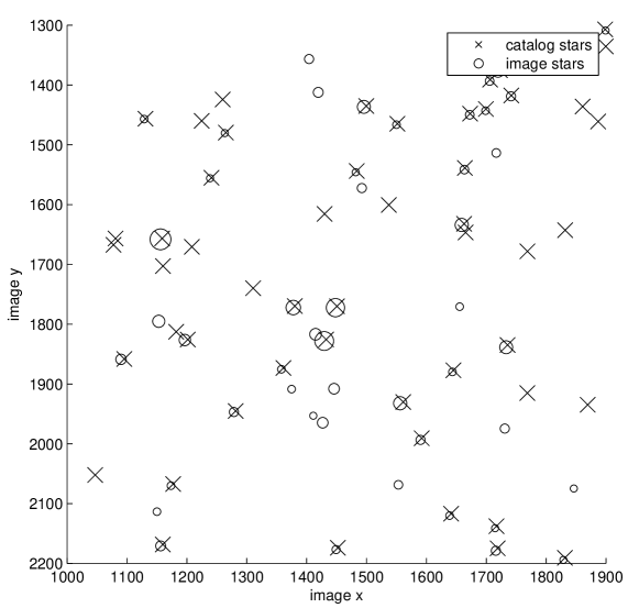
(a) Catalog at year 1914, initial image.

(b) Catalog at year 1914, fitted image.

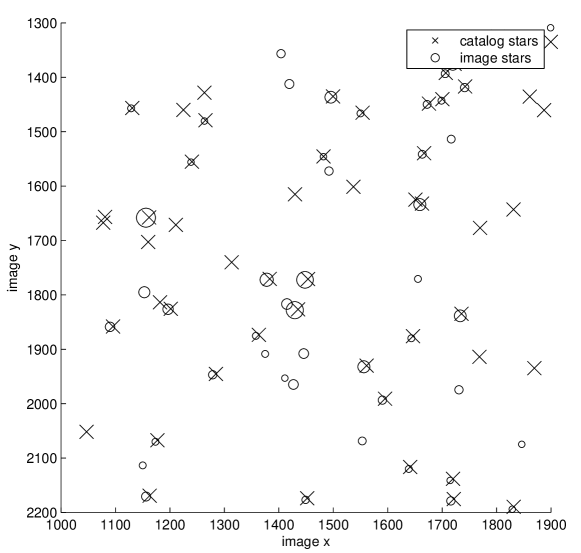
(c) Catalog at year 2000, initial image.

(d) Catalog at year 2000, fitted image.

Figure 2: The extracted sources (size is proportional to brightness) from the 900 by 900 pixel sub-image shown in Figure 5. These plots illustrate the error in the initial calibration returned by the Astrometry.net solver, as well as the difference in fitting a historical image to USNO-B Catalog at the year 2000 and to the Catalog at 1914, the year which we correctly estimate to be the image’s year of origin.

See Figure 2 for some examples of fit and unfit images against correct and incorrect catalog dates.

3.4 Estimating the date

Now that we have defined a method for fitting an image to the catalog, and a metric by which we can assess the degree to which an image can be fit to the catalog, we can use a number of techniques to estimate the year in which the image can best be fit to the catalog. We take that year to be the year in which the image was created.

This problem can be phrased as such: an image has some unknown chi-squared curve $\chi^{2}(t)$, of which we wish to find the year $t_{0}$, the theoretical optimal year such that:

$$t_{0}=\underset{t}{\arg\min}\,\chi^{2}(t)$$ (20)

In the algorithm we will describe, finding $t_{0}$ is not computationally feasible, so we must settle on finding a reasonable approximation of the minimum $t^{*}$, such that given an accuracy threshold $\delta_{\chi}$ we are confident that:

$$\left|\left|\chi^{2}(t_{0})-\chi^{2}(t^{*})\right|\right|\leq\delta_{\chi}$$ (21)

Once we have found $t^{*}$ and therefore $\chi^{2}(t^{*})$, we also wish to find the extents of our uncertainty region, $(t^{*}_{-},t^{*}_{+})$, such that:

$$\begin{array}[]{c}t^{*}_{-}<t^{*}<t^{*}_{+}\vskip 6.0pt plus 2.0pt minus 2.0pt\\ \chi^{2}(t^{*}_{-})=\chi^{2}(t^{*})+1=\chi^{2}(t^{*}_{+})\vskip 6.0pt plus 2.0pt minus 2.0pt\\ \underset{t\in[t^{*}_{-},t^{*}_{+}]}{\forall}{\,\chi^{2}(t)\leq\chi^{2}(t^{*})+1}\end{array}$$ (22)

Ideally, we want to find all of these values as accurately as possible while sampling the $\chi^{2}$ curve as few times as possible. There are a number of methods by which we can accomplish this task, each with different tradeoffs concerning efficiency and assumptions about the shape of the curve.

The simplest method for estimating the origin date is through brute force. We sample our $\chi^{2}$ curve at regular intervals, and take the year in which our objective function scored the lowest as $t^{*}$. We then linearly interpolate along the curve to find the extents of the uncertainty region. This method is terribly inefficient and assumes nothing about the shape of the curve, so we only use it as an approximate ground truth to which we will compare our final algorithm.

Our search algorithm begins with first sampling our $\chi^{2}$ curve at a very broad, regular interval. Though only one initial sample is required, for the figures shown in this paper we sample the curve at $1900$, $1950$, and $2000$. We take the sampled year with the lowest $\chi^{2}$ score to be $t_{n}$, and we then iteratively refine $t_{n}$ into $t_{n+1}$ until we believe that we have found $t^{*}$.

Our objective function was constructed such that we could efficiently calculate $\frac{\mathrm{d}\chi^{2}}{\mathrm{d}t}(t)$ and $\frac{\mathrm{d}^{2}\chi^{2}}{\mathrm{d}t^{2}}(t)$. The equations for these analytical derivatives are elaborate, so we do not present them here. Since $\chi^{2}(t^{*})$ is a minimum in the $\chi^{2}$ curve, we can assume that $\frac{\mathrm{d}\chi^{2}}{\mathrm{d}t}(t^{*})=0$. We can therefore use Newton’s method to find $t_{n+1}$:

$$t_{n+1}=t_{n}-\frac{\frac{\mathrm{d}\chi^{2}}{\mathrm{d}t}(t_{n})}{\frac{\mathrm{d}^{2}\chi^{2}}{\mathrm{d}t^{2}}(t_{n})}$$ (23)

We iteratively evaluate $t_{n+1}$ until $\left|\left|\chi^{2}(t_{n+1})-\chi^{2}(t_{n})\right|\right|\leq\delta_{\chi}$ holds for two consecutive iterations, at which point we take $t_{n+1}$ as $t^{*}$. Since Newton’s method generally converges quadratically, this is an extremely fast process.

Once we have found $t^{*}$, we can locate $t^{*}_{-}$ and $t^{*}_{+}$. We use our modified Newton’s method with these new goals:

$$\displaystyle\chi^{2}(t^{*}_{+})=\chi^{2}(t^{*})+1$$

$$\chi^{2}(t^{*}_{-})=\chi^{2}(t^{*})+1$$ (24)

This uncertainty region would be the true one-sigma uncertainty region in the limit that the modified chi-squared were the standard linear-fitting chi-squared. Because of the weighting function, in practice this criterion over-estimates the one-sigma uncertainty.

We can perform root-finding on these equations using the following formula for iteration:

$$t_{n+1}=t_{n}-\frac{\chi^{2}(t_{n})-\left(\chi^{2}(t^{*})+1\right)}{\frac{\mathrm{d}\chi^{2}}{\mathrm{d}t}(t_{n})}$$ (25)

We begin our two new searches with a sensible initial estimate of the bounds of the uncertainty region, based on our present knowledge of the $\chi^{2}$ curve. These searches operate under all of the constraints under which the previously detailed search operated, and also converges when $\left|\left|\chi^{2}(t_{n+1})-\chi^{2}(t_{n})\right|\right|\leq\delta_{\chi}$ holds for two consecutive iterations.

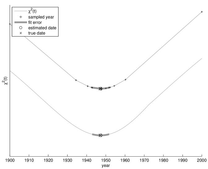
Figure 3: Evaluation of the accuracy of our search algorithm. The top is our modified Newton’s method with $\delta_{\chi}=10^{-4}$, and the bottom is brute force, with an interval of $0.1$ years. The uncertainty regions are identical to within $10^{-3}$ years, and the estimated dates are within $0.05$ years of each other. Brute force took 1001 iterations to achieve this accuracy, while Newton’s method took only 23. For clarity’s sake, the curves were vertically separated, and the individual points that were sampled to construct the brute-force curve are not displayed.

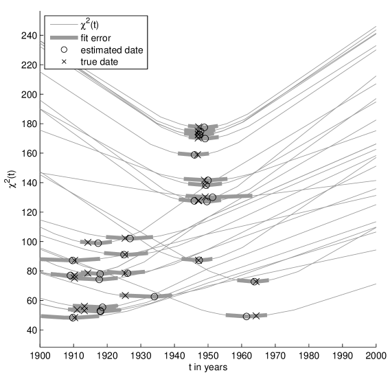
(a) Estimated $\chi^{2}$ curves of the science-quality images.

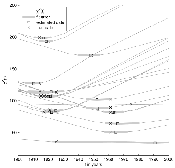
(b) Estimated $\chi^{2}$ curves of the low-quality images.

Figure 4: The estimations of each image’s $\chi^{2}$ curves generated by our modified Newton’s method, for both datasets. The vertical axes of these plots do not show the constant contributions of image–catalog pairs whose separations are always too large to be directly calculated, as including those would make the curves excessively vertically separated, rendering these plots incomprehensible.

Additionally, we can speed up the total search process by using the transformed image points from the previous iteration to find the new transformation for the next iteration. This heuristic means that as the search converges on a final result, the amount of time required to query new years is dramatically reduced. Also, it becomes easier to visualize the search algorithm as a single bidirectional fitting process, in which we repeatedly fit the image to the catalog and the catalog to the image until both fittings have converged. Just as in the previous section, all transformations are constructed using the initial positions of the points, so our final transformation after searching the $\chi^{2}$ curve is still very numerically stable. Figure 3 shows a comparison of this search algorithm against a brute-force “ground truth”. Figure 4 shows the modified $\chi^{2}$ curves for each image as they were estimated by this search algorithm.

The output of this process is a polynomial description of the image astrometric WCS, a best-fit year value $t^{*}$, and an uncertainty region around that value.

3.5 Implementation notes

Blind Date’s two primary performance bottlenecks are calculating the distances between image and catalog points and solving the weighted least-squares problems. In both cases, we are able to use the properties of our weighting function to construct approximate solutions that very effectively approximate the true solution.

Our algorithm theoretically requires us to repeatedly calculate the distances of all image–catalog pairs. However, due to the properties of the weighting function as described in Section 3.2, we do not need to know the distances of significantly separated pairs. Because the transformation applied at each iteration tends to be very small, we can generally assume that significantly separated pairs in one iteration will also be significantly separated in the next iteration. This allow us to do one initial calculation of all image–catalog distances, but in later iterations only calculate the distances of image–catalog pairs that will likely cause a change in the value of the objective function. This is a rough heuristic, so we safeguard ourselves by manually recalculating all image–catalog distances every 10 iterations, as well as whenever the IRLS begins to converge. This dramatically speeds up our algorithm, while producing nearly identical results to the naïve brute-force approach.

We use the aforementioned properties of our weight function to determine if an image–catalog pair should be considered in the weighted least-squares calculation. A highly separated pair always contributes a nearly-constant value to the residuals, and therefore can be safely ignored. This gives us a slight performance boost.

We require an additional threshold for the difference between the optimal function from one iteration to the next, which determines when our IRLS operation has converged. We use the very conservative value of $10^{-4}$ as the maximum amount that the $\chi^{2}$ score of the final IRLS iteration is allowed to change from those of the previous two IRLS iterations.

4 Results

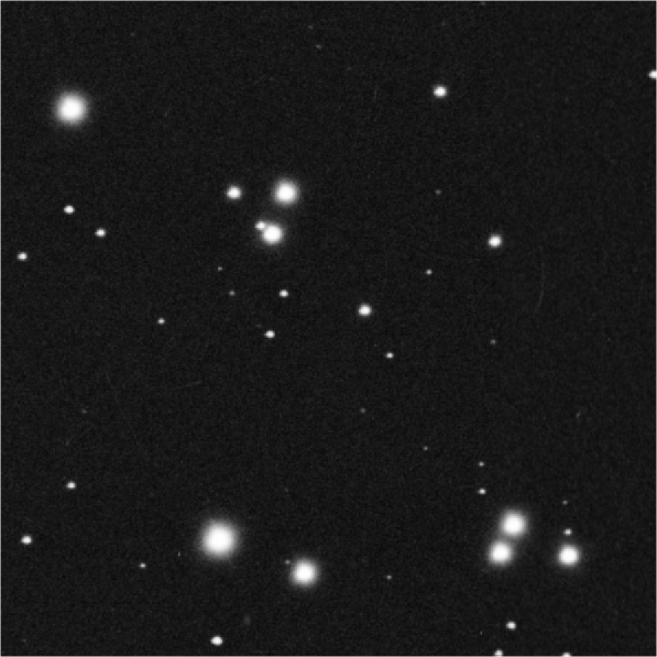
(a) Mar-1914 / Nov-1917

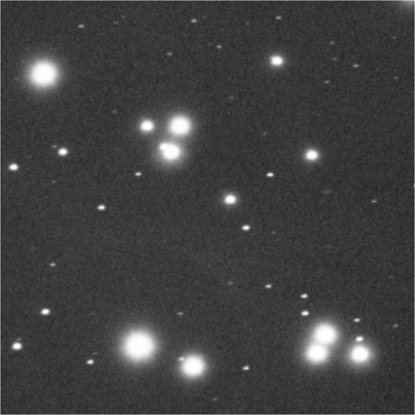
(b) Mar-1947 / Nov-1945

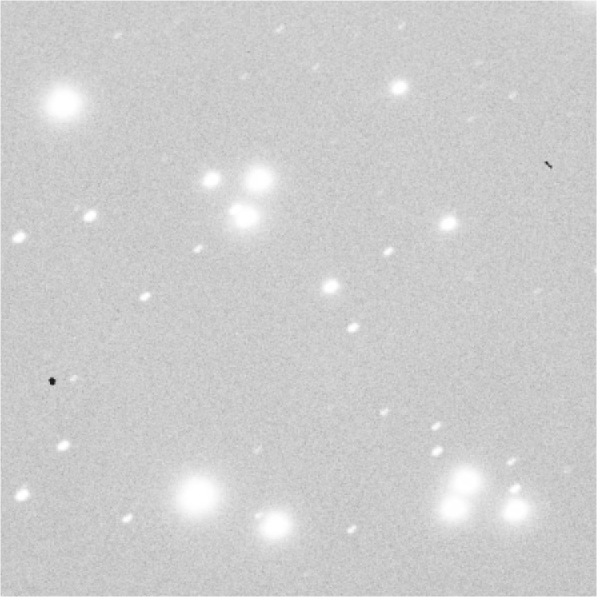
(c) Feb-1949 / May-1951

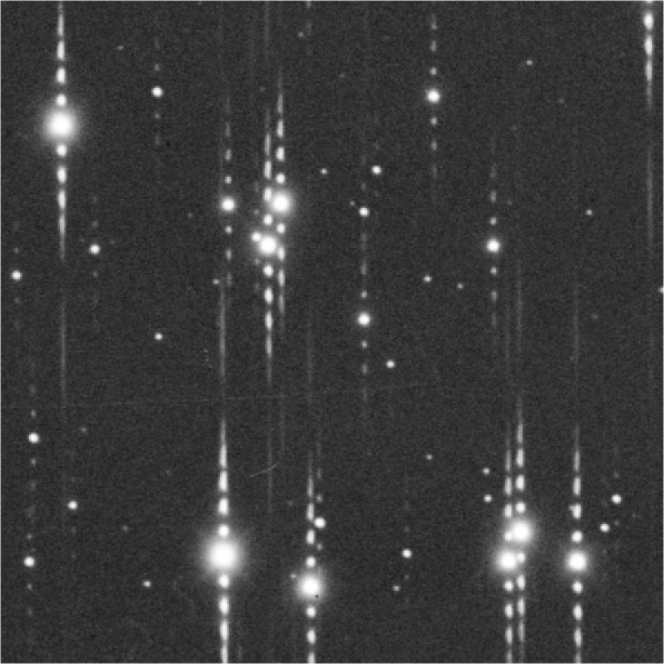
(d) Feb-1914 / Jun-1910

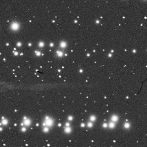
(e) Mar-1914 / Nov-1916

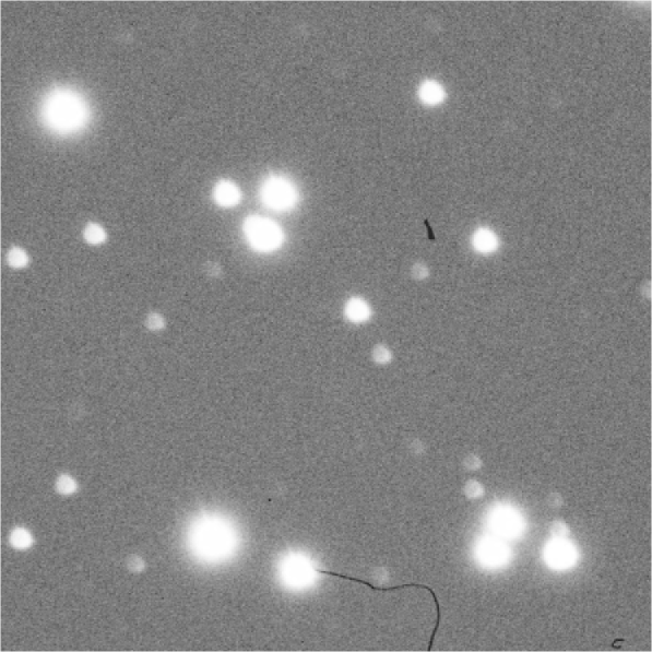
(f) Jan-1975 / Jan-1800

Figure 5: A series of $900$ by $900$ pixel subsets of our $3000$ by $3000$ pixel images. The top three images are from our set of science-quality images, and the the bottom three images are from our set of low-quality images. The captions are of the form “true date / estimated date”. All but figure 5(f) have estimated dates that lie within the uncertainty region.

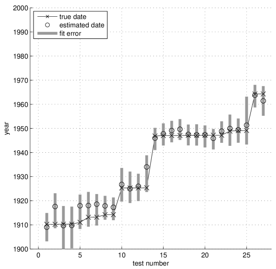
(a) Performance on the science-quality images.

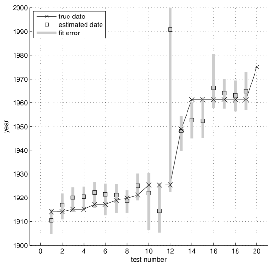
(b) Performance on the low-quality images.

Figure 6: An informative visualization of performance for both datasets. The x-axis is an arbitrary index denoting the test image (images were sorted by true year), and the y-axis shows each image’s true year, estimated year, and uncertainty region. The last image in figure 6(b) is not shown, as it is estimated as originating before $1900$.

Harvard’s interface for accessing its scanned plates of M44 made it difficult to obtain more than $3000$ by $3000$ pixel subsets of the images, though the entire plates are significantly larger. The interface for downloading the images did not provide an obvious mechanism for selecting the same $3000$ by $3000$ pixel subsets of each image, which means that such selection was done by hand, and is therefore not very accurate. Many of the plates suffer from the many sources of noise typical of historical imagery: Some are multiple-exposures, badly out of focus, badly saturated, or cracked, and some contain handwritten labels, digital scanning artifacts, and bad trailing. For the sake of fairly assessing Blind Date’s performance, we split the images into two sets; 27 “science-quality” images and 20 “low-quality” (see Figure 5 for examples). For our convenience, we used the JPEG versions of the images, which probably introduces some minor noise in the form of compression artifacts. Harvard graciously provided ground-truth dates for each image, which presumably were taken from logs or from writing on the plates. We take these dates to be true. Though the ground-truth dates range from 1910 to 1975, the dates are not uniformly distributed. See the distribution of images along the y-axis of figure 6 for a demonstration of this clustering.

The tests were performed using the modified Newton’s method, with affine distortions and an accuracy threshold $\delta_{\chi}$ of $10^{-4}$ year. Tests were done on a 2007 Macbook with a 2GHz Intel Core 2 Duo processor, and 2GB of RAM. Median runtime for estimating each image’s date was $\sim 2.6$ seconds per image, after source extraction and Astrometry.net’s initial calibration. Results are shown in Table 1.

	mean year error (bias)	median absolute error	fraction within uncertainty
science-quality	$1.68$	$1.29$	$27/27$
low-quality	$-5.28$	$4.00$	$17/20$

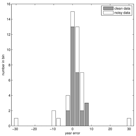
(a) Error in date estimation.

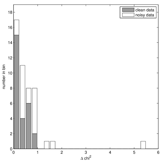
(b) Error relative to uncertainty.

Figure 7: Histograms of the errors in date estimation, for both datasets. Figure 7(a) shows the difference between our estimated dates and the true dates. Figure 7(b) shows those errors relative to the widths of the uncertainties; effectively, the differences between the $\chi^{2}$ scores of the true years and the $\chi^{2}$ scores of the estimated years. A relative error of less than $1$ indicates that the true year lies within the uncertainty. The two outliers in figure 7(a) are actually significantly worse than they appear: $+65$ and $-175$ years.

Table 1: Accuracy of estimated dates for the two subsets of data. See Figures 6 and 7 for a more detailed visualization of the results.

Though the results shown were generated by fitting an affine (linear) transformation in image coordinates, we experimented with increasing the order of the polynomial warp being fitted. Results were very similar to those obtained using affine transformations, although the median absolute error for science-quality images dropped to $1.01$ years for second-order transformation, and to $0.99$ years for third-order transformations. Median absolute error for low-quality images also decreased slightly as the order was increased, as did the bias for science-quality images.

Additionally, we tested Blind Date on the five USNO-B Catalog source images of M44 that we were able to retrieve from the US Naval Observatory Precision Measuring Machine Data Archive, and on the Sloan Digital Sky Survey (York et al, 2000) image of M44. The dates of the USNO-B Catalog source imagery were estimated accurately (all within six years of the true dates, and all within the uncertainties), which is as good as we would expect performance to be given the relatively low resolution ($3.2\,\mathrm{arcsec}\,\mathrm{pix}^{-1}$) of the source imagery that we were able to obtain. The SDSS image was estimated to have been taken in late 2004, and was actually taken in 2006.

We assembled an alternate test-bed of ten amateur images of M44 that we were able to find online. The websites on which we found most of our imagery did not explicitly note the date at which the image was taken, so we were forced to use the “date” tag in each image’s EXIF meta-data as the ground truth. For many of the images, Blind Date provided accurate dates and uncertainties that are consistent with our previous findings: all estimated dates lay within the our uncertainty bounds, accuracy generally depended on the resolution and quality of each image, and most estimated dates (for all sufficiently high-resolution images) were within a few years from the true dates. Our ground-truth dates are, unfortunately, very unreliable, as the EXIF data may simply reflect the date at which an image was digitized or modified, rather than the date at which it was imaged. Though this means that we are not able to truly vet Blind Date’s performance for these amateur images, this issue also highlights the utility of this system: the dates of origin of these images are effectively lost, but can be re-estimated.

5 Discussion

We have shown that our Blind Date system can successfully attach time meta-data to historical imaging data. The system runs in seconds on standard inexpensive consumer computer equipment; it does not require large investments of time or money to vet or create time meta-data for large collections of astronomical imaging.

The performance of Blind Date will depend on the properties of the input image, and on the properties of the catalog information known about the region of the sky that is being imaged. We can phrase this as two questions: “What is the information content in an image?”, and “What is the information content in a catalog star?”

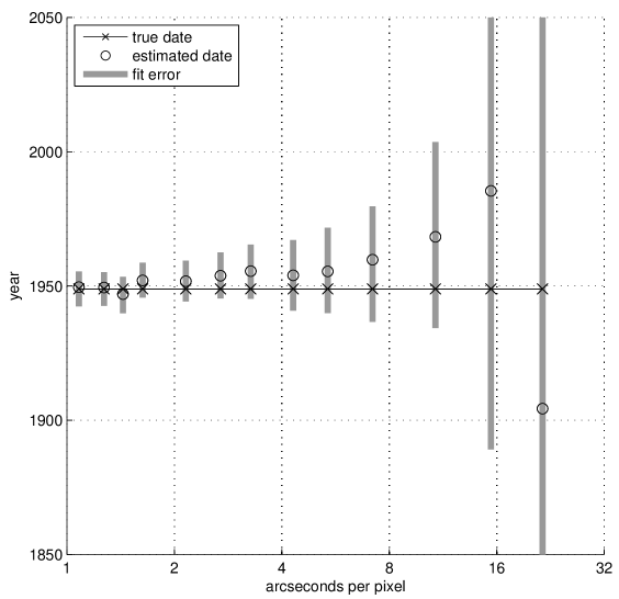
(a) Performance versus resolution.

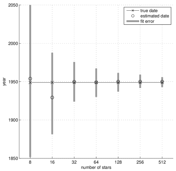
(b) Performance versus number of image stars.

Figure 8: Plots showing performance relative the resolution of the input image, and to the number of stars the input image contains. Figure 8(a) was produced by repeatedly downsampling the input image, while Figure 8(b) was produced by repeatedly cropping out the borders of the input image. Note that in downsampling the image, some smaller stars stop being detectable by our source-extraction algorithm, so the number of stars in the image decreases with the resolution of the image.

In an attempt to empirically assess the information content of an image, we ran a simple experiment in which we varied the resolution of an input images and the number of stars contained in an input image (by downsampling and cropping the image, respectively). The results are shown in Figure 8, where we see that performance depends heavily on an image containing a large number of stars imaged at high resolution. We also explored the effects of different kinds of imaging defects. Our objective function is designed to be robust to false sources, and as such, Blind Date performs very well on images with multiple exposures. Our experiments suggests that saturation, large PSF due to poor focus or trailing, and short exposure time (low sensitivity) most negatively effect Blind Date’s performance. See Figure 5 for examples of our accuracy in the face of different kinds of imaging defects. Trailing and saturation can effectively be thought of as decreasing the resolution of our input image (by decreasing our ability to accurately centroid stars), and shallow imaging is effectively equivalent to dropping dim stars out of the image; these are the two trends demonstrated in Figure 8. Once again, Blind Date’s accuracy appears to depend on an image containing many well-imaged (high resolution) stars.

The information in a single catalog star (provided that it has been detected in the input image, in the limit that our procedure is equivalent to least-square fitting) is proportional to that star’s contribution to the second derivative of $\chi^{2}$ with respect to date. This contribution is approximately the square of the magnitude of the star’s proper motion, divided by the square of the uncertainty, that is, the square of the signal-to-noise at which the proper motion is detected (where the “noise” in this case is the combined uncertainty from the catalog and the image as in equation 3). We expect Blind Date’s performance on an image to scale roughly with the sum of the squares of the detected catalog stars’ proper motion signal-to-noise ratios. Imagery unlike the imagery analyzed here ought to obtain date calibration with uncertainty that goes down as the sum of the detected catalog stars’ proper motion signal-to-noise ratios goes up.

Increasing the polynomial order of the transformation on the image plane produces slightly more accurate date estimates, presumably because the input images do have distortions that are represented reasonably by these functions. We are reluctant to advocate unnecessarily large polynomial orders, as—theoretically—the more freedom we give the transformation model, the more irregular our resulting $\chi^{2}$ curves may become. That being said, we have not seen any evidence that reinforces such a concern. In principle, even more accurate results could be obtained without increasing the number of degrees of freedom in the fit by employing a physical camera model that represents known distortions in the particular camera used to take the data.

For each image in our dataset, we performed an experiment to determine the range of initial dates for which our search algorithm is robust. We discovered each image had a range of at least $300$ years (and on average, $620$ years) roughly centered around the true year from which the search could be initialized without the final result being affected. If we ignore our precaution of using gradient descent when the second derivative of the $\chi^{2}$ curve is non-positive, this range is significantly smaller (on average, about $55$ years). This finding highlights the importance of the modifications we make to Newton’s method in constructing our search algorithm, and also suggests that the coarse grid of queries with which we initialize our search is unnecessary—a single initial query in the correct century would have been more than sufficient.

Blind Date largely ignores one very important source of information, namely the brightnesses of the image and catalog stars. This data is used in our band-pass estimation step, but is then largely ignored. In future versions of Astrometry.net we plan to utilize this data in a number of ways. We eventually hope to simultaneously estimate all parameters of a given image, including the image’s WCS, its date of origin, and its band-pass. Estimating all of these simultaneously should means that brightness information is implicitly used in our estimation of the location and date, and should improve our results accordingly. This would also solve our current conundrum regarding this process, which is that image–catalog correspondences are required for band-pass estimation, while band-pass estimation is required for finding image–catalog correspondences.

Analysis of the brightness of image stars may be able to play a profound role in date estimation if we consider the subset with periodic variability. Given an image containing $k$ stars with different periods, and given sufficient information concerning the periodic variations in their brightnesses, we should be able to constrain the date of origin of the image to one of a set of time intervals in which those $k$ stars are at whatever particular point in their periods (to within photometric precision). Given the set of intervals constrained by the periodic variations, we can use the range of dates determined by Blind Date (that is, from the proper motions of the stars) to select a potentially very narrow time interval in which the image must have originated. In principle, it may even be possible to determine the date of origin of an image solely though periodic brightness, though that would require very good measurements of the periods of the catalog stars and of the brightnesses of the image stars.

Blind Date’s value, on the most superficial level, is clear: this system could be used to recover lost meta-data (at low precision) for historical and amateur data that have been archived poorly or not at all. Now that large scanning projects are underway at photographic archives and the web is providing new opportunities for file sharing among amateurs and professionals, we need systems that automatically vet and provide meta-data for data of unknown provenance.

Regardless of whether or not imagery already contains reliable date meta-data, the techniques described in Blind Date may have deep-seated implications for the calibration of all imagery not taken at the year $2000.0$. The fact that the date can be well estimated from input images demonstrates both that the images contain important information about stellar motions, and that astrometric calibration is hampered when calibration is performed with a catalog projected to an epoch far from the date of the image. A system that is time sensitive, such as Blind Date, will plausibly provide the best astrometric calibration possible for arbitrary imaging.

What may be Blind Date’s most important consequence is an inversion of the system, in which we attempt to use imagery to re-estimate the proper motions of catalog stars. The most straightforward approach to this would be to “cheat” and use the ground-truth dates of all input imagery. One could repeatedly: calibrate each image using the catalog wound to that image’s date-of-origin, re-estimate the proper motions of the catalog stars, and re-wind the catalog using those new proper motions. This could be thought of as performing expectation-maximization on the proper motions of the catalog. Of course, an ideal system would be robust to some (or all) input imagery not having ground-truth ages. We could estimate the date-of-origin of all unlabeled imagery, and use these estimates (and their uncertainties) in our expectation-maximization. Labeled and unlabeled data could be treated equivalently, except that labeled data would have much less uncertainty associated with it. This system would then become a two-way street, in which we do not just reposition images relative to the sky, but also reposition the sky relative to the images, and dynamically develop a consensus between the two. The future Astrometry.net “catalog” would not have to be a static entity, but would instead be a consensus of all available imagery—using the USNO-B Catalog as a static “prior.” Blind Date takes us one step closer to this grand long-term hope for Astrometry.net becoming an always-changing database of everything we know about the sky, by allowing time to become one more dimension of our data.

References

- Barron et al (2008) Barron, J. T., Stumm, C., Hogg, D. W., Lang, D., & Roweis, S., 2008, AJ, 135, 414
- Hampel et al (1986) Hampel, F. R., Ronchetti, E. M., Rousseeuw, P. J., & Stahel, W. A., 1986, Robust Statistics: The Approach Based on Influence Functions, Wiley, New York
- Lang et al (2008) Lang, D., Hogg, D. W., Mierle, K., Blanton, M., & Roweis, S., 2007, Science, submitted
- Monet et al (2003) Monet, D. G., et al, 2003, AJ, 125, 984
- York et al (2000) York, D., et al, 2000, AJ, 120, 1579