Efficient $\mathcal{O}(N^{2})$ approach to solve the Bethe-Salpeter equation for excitonic bound states

Abstract

Excitonic effects in optical spectra and electron-hole pair excitations are described by solutions of the Bethe-Salpeter equation (BSE) that accounts for the Coulomb interaction of excited electron-hole pairs. Although for the computation of excitonic optical spectra in an extended frequency range efficient methods are available, the determination and analysis of individual exciton states still requires the diagonalization of the electron-hole Hamiltonian $\hat{H}$. We present a numerically efficient approach for the calculation of exciton states with quadratically scaling complexity, which significantly diminishes the computational costs compared to the commonly used cubically scaling direct-diagonalization schemes. The accuracy and performance of this approach is demonstrated by solving the BSE numerically for the Wannier-Mott two-band model in k space and the semiconductors MgO and InN. For the convergence with respect to the ${\bf k}$-point sampling a general trend is identified, which can be used to extrapolate converged results for the binding energies of the lowest bound states.

I Introduction

The Coulomb interaction of excited electrons and holes plays an important role for the optical properties of condensed matter Sham and Rice (1966); Hanke and Sham (1979); Strinati (1988). Photon-induced two-particle electronic excitations are accompanied by the rearrangement of the remaining electrons in a solid, so that the individual particles are renormalized to quasiparticles (QPs). Their description within the framework of many-body perturbation theory (MBPT) has made substantial progress in the last three decades Onida et al. (2002). The most common approach is Hedin’s GW approximation Hedin (1965), which describes the response of the remaining electrons by a dynamically screened Coulomb potential $W$. The self-energy operator $\Sigma$ of an excited particle is thereby given by $\Sigma=i\hbar GW$ with the single-particle Green’s function $G$. Its numerical implementation Hybertsen and Louie (1985); Godby et al. (1987) usually yields single-particle excitation energies in good agreement with angle-resolved or inverse photoemission experiments Bechstedt (1992); Aryasetiawan and Gunnarsson (1998); Aulbur et al. (2000). However, the optically excited quasielectron-quasihole pairs show additional interactions. They are described by the so called polarization function $P$, which obeys a Bethe-Salpeter equation (BSE) Sham and Rice (1966); Hanke and Sham (1979). Apart from the bare electron-hole exchange, which can be identified with crystal local-field effects (LFEs) Hanke and Sham (1979), its kernel is given by the derivative $-(i\hbar)^{-1}\delta\Sigma/\delta G$ which is usually replaced by the leading term $-W$. It clearly represents the screened Coulomb attraction between quasielectrons and quasiholes Strinati (1988).

Optical spectra of real materials can be calculated from first principles by solving the eigenvalue problem (EVP) for an effective two-particle Hamiltonian $\hat{H}$ corresponding to a reformulated BSE. The eigensystem of $\hat{H}$ then can be used to obtain a spectral representation of $P$. Usually, one of the following numerical approaches is applied to calculate $P$ or the directly related frequency-dependent dielectric function $\epsilon(\omega)$: (i) The explicit diagonalization of $\hat{H}$ (solving the EVP directly Albrecht et al. (1998); Rohlfing and Louie (1998a)), (ii) the iterative Haydock method Benedict et al. (1998), or (iii) a time-evolution algorithm that is based on an initial-value formulation of the Fourier-transformed dielectric function Schmidt et al. (2003). Meanwhile, the applications extend also to rather complex materials and structures such as semiconductor surfaces Rohlfing and Louie (1999); Hahn et al. (2002), nanocrystals and molecules Rohlfing and Louie (1998b); Hahn et al. (2005a), or even ice and water Hahn et al. (2005b); Garbuio et al. (2006). The most important changes in the optical spectra with respect to the independent-particle limit concern a general redshift of the transition energies and a redistribution of oscillator strength towards lower energies Schmidt et al. (2003).

For some systems also bound states of the electron-hole pairs – so called excitons Kittel (1996) – form and can be observed in optical spectra below the QP absorption edge. Thereby, two fundamentally different types of excitons – the Frenkel and the Wannier-Mott type – are distinguished. Excitons of the Frenkel type emerge in systems where the gap is confined by rather localized electronic states, as it is found for surfaces of covalently bonded semiconductors Rohlfing and Louie (1999), insulators with strong ionic bonds Rohlfing and Louie (1998a); Benedict et al. (1998); Benedict and Shirley (1999); Bechstedt et al. (2005), or crystals with hydrogen-bridge bonds Hahn et al. (2005c). For materials with a pronounced dispersion of the first conduction band excitons of the Wannier-Mott type Kittel (1996); Yu and Cardona (1999); Elliott (1957); Shinada and Sugano (1966) can form below the gap. They give rise to a hydrogen-like spectrum of pair eigenvalues and, in contrast to the Frenkel type, an electron-hole distance much larger than the lattice constant. Typically, their binding energies are much smaller than those of Frenkel-like excitons. Nevertheless, the lowest excitonic states can be probed by a variety of spectroscopic techniques.

However, first-principles calculations, as outlined above, remain a challenging task especially for Wannier-Mott-like excitons with binding energies below 0.1 eV. The most important limitation is due to the high ${\bf k}$-point densities required for sampling the Brillouin zone (BZ), in order to describe the localization of the excitonic wave function in the Fourier space sufficiently. The number of ${\bf k}$ points directly relates to the rank $N$ of the BSE Hamiltonian, causing extreme demands in terms of storage and CPU time for the calculation of the spectra. The latter one rapidly becomes the limiting factor, since, of the previously discussed approaches, only the direct diagonalization of $\hat{H}$ – involving computational costs scaling like $\mathcal{O}(N^{3})$ – can be employed in the computation of bound pair excitations. Attempts have been made to solve the problem by introducing an interpolation scheme for the electron-hole interaction Rohlfing and Louie (2000) or by ${\bf k}$-point samplings restricted to only a small part of the BZ Laskowski et al. (2005); Laskowski and Christensen (2006). Still, the question how the complete electronic structure influences the bound pair excitations and their the oscillator strengths remains open. Also the effects of electron-hole exchange on the excitons Denisov and Makarov (1973); Fu et al. (1999) have been studied little so far by a combination of ab initio electronic structure calculations and the BSE treatment of the two-particle excitations. Another important point concerns the prediction of excitonic effects, e.g. binding energies and oscillator strengths, for semiconductors such as InN, whose sample quality does currently not allow their measurement. Also the influence of polytypism of a material remains an open question.

In order to reduce the computational demands necessary for systematic studies addressing the aforementioned questions, we combine the use of special ${\bf k}$-point sets and an iterative matrix-diagonalization scheme, obtaining a computationally very efficient approach for the calculation of excitonic states below the absorption edge. The methodology of this approach is described in detail in Sec. II. The computational details of the underlying ab initio calculations are summarized in Sec. III, before in Sec. IV.A the approach is applied to and tested by means of the Wannier-Mott model exciton. The consequences of ”true” ab initio band structures are studied for the semiconductors MgO and InN in Sec. IV.B and C. Finally, a summary and conclusions are given in Sec. V.

II Methodology

II.1 Bethe-Salpeter equation and pair Hamiltonian

The inclusion of excitonic effects in optical spectra requires to go beyond the independent-(quasi)particle approximation (IQA) for the polarization function $P$ by taking into account the electron-hole attraction and exchange. For this purpose a BSE for the irreducible polarization can be derived from MBPT Sham and Rice (1966); Onida et al. (2002),

$$P=P_{0}+P_{0}(2\bar{v}-W)P,$$ (1)

with the IQA polarization function $P_{0}$, the statically screened Coulomb potential $W$, and the bare Coulomb potential $\bar{v}$ without its long-range Fourier component ${\bf G}=0$. For a detailed derivation and a generalization for collinear spin polarization we like to refer to Rödl et al. (2008).

A commonly adopted basis for representing the BSE is given by the Bloch states $\varphi_{n{\bf k}}({\bf r})$ of the crystal problem, characterized by the band index $n$ and a wave vector of the first BZ ${\bf k}$. Neglecting QP effects for the wave functions, they are usually approximated by the wave functions obtained in the framework of density functional theory (DFT) from the solution of the Kohn-Sham equation,

$$\left[-\frac{\hbar^{2}}{2m}\Delta+V({\bf r})+V_{H}({\bf r})+V_{XC}({\bf r})\right]\varphi_{n{\bf k}}({\bf r})=\varepsilon_{n}({\bf k})\varphi_{n{\bf k}}({\bf r}),$$ (2)

with the Kohn-Sham eigenvalues $\varepsilon_{n}({\bf k})$ and the potentials of electron-ion ($V$), Hartree ($V_{H}$), and exchange and correlation (XC, $V_{XC}$) interaction. The latter potential is usually given by the local-density (LDA) or generalized-gradient approximation (GGA). However, for materials where these approximations fail, such as InN, other potentials derived, e.g. from the LDA+U scheme Anisimov et al. (1991) or even spatially non-local potentials in the framework of generalized Kohn-Sham schemes Seidl et al. (1996) might be used. Especially the latter constitute a good starting point for the pertubative calculation of single-particle QP eigenvalues $E^{QP}_{n}({\bf k})$ Fuchs et al. (2007).

With restriction to materials with completely occupied and unoccupied bands (semiconductors and insulators), the BSE (1) can be rewritten as EVP for an effective two-particle Hamiltonian $\hat{H}$ Albrecht et al. (1998),

$$\frac{\Omega}{(2\pi)^{3}}\sum_{c^{\prime}v^{\prime}}\int_{\Omega_{BZ}}d{\bf k}^{\prime}\hat{H}^{c}_{c^{\prime}}{}^{v}_{v^{\prime}}({\bf k},{\bf k}^{\prime})A^{\Lambda}_{c^{\prime}v^{\prime}}({\bf k}^{\prime})=E^{\Lambda}A^{\Lambda}_{cv}({\bf k}),$$ (3)

with the pair eigenvalues $E^{\Lambda}$ and eigenvectors $A^{\Lambda}_{cv}({\bf k})$, $\Omega$ the crystal volume, and $\Omega_{BZ}$ the volume of the BZ. The two-particle Hamiltonian can be divided into a diagonal and a non-diagonal part,

$$\hat{H}^{c}_{c^{\prime}}{}^{v}_{v^{\prime}}({\bf k},{\bf k}^{\prime})=H^{D}_{cv}({\bf k})\delta_{vv^{\prime}}\delta_{cc^{\prime}}\delta_{{\bf k}{\bf k}^{\prime}}+H^{c}_{c^{\prime}}{}^{v}_{v^{\prime}}({\bf k},{\bf k}^{\prime}),$$ (4)

with

$$H^{D}_{cv}({\bf k}) =E^{QP}_{c}({\bf k})-E^{QP}_{v}({\bf k}),$$ (5a)

$$H^{c}_{c^{\prime}}{}^{v}_{v^{\prime}}({\bf k},{\bf k}^{\prime}) =-W^{c}_{c^{\prime}}{}^{v}_{v^{\prime}}{}^{{\bf k}}_{{\bf k}^{\prime}}+2\bar{v}^{c}_{c^{\prime}}{}^{v}_{v^{\prime}}{}^{{\bf k}}_{{\bf k}^{\prime}},$$ (5b)

where $\delta_{{\bf k}{\bf k}^{\prime}}$ is used as short notation for $(2\pi)^{3}\Omega^{-1}\delta({\bf k}-{\bf k}^{\prime})$. The first, diagonal, contribution to (4) is constructed from the difference of the QP eigenvalues of conduction and valence bands. It describes the excitation of non-interacting quasiparticles. The second part, given by the matrix elements of the statically screened Coulomb potential $W$, accounts for the attraction of electrons and holes,

$$\begin{split}W^{c}_{c^{\prime}}{}^{v}_{v^{\prime}}{}^{{\bf k}}_{{\bf k}^{\prime}}&=\!\!\iint\!d{\bf r}d{\bf r}^{\prime}\,\varphi^{*}_{c{\bf k}}({\bf r})\varphi_{c^{\prime}{\bf k}^{\prime}}({\bf r})W({\bf r},{\bf r}^{\prime})\varphi_{v{\bf k}}({\bf r}^{\prime})\varphi^{*}_{v^{\prime}{\bf k}^{\prime}}({\bf r}^{\prime})\\ &=\frac{1}{\Omega}\sum_{{\bf G}{\bf G}^{\prime}}\frac{4\pi e^{2}\epsilon^{-1}_{{\bf G}{\bf G}^{\prime}}({\bf k}-{\bf k}^{\prime})}{|{\bf k}-{\bf k}^{\prime}+{\bf G}||{\bf k}-{\bf k}^{\prime}+{\bf G}^{\prime}|}B^{c}_{c^{\prime}}{}^{{\bf k}}_{{\bf k}^{\prime}}({\bf G})B^{v}_{v^{\prime}}{}^{{\bf k}*}_{{\bf k}^{\prime}}({\bf G}^{\prime}),\end{split}$$ (6)

with the symmetrized inverse dielectric function $\epsilon^{-1}_{{\bf G}{\bf G}^{\prime}}$ and the Bloch integrals

$$B^{n}_{n^{\prime}}{}^{{\bf k}}_{{\bf k}^{\prime}}({\bf G})=\frac{1}{\Omega_{0}}\int_{\Omega_{0}}d{\bf r}\,u^{*}_{n{\bf k}}({\bf r})e^{i{\bf G}{\bf r}}u_{n^{\prime}{\bf k}^{\prime}}({\bf r}).$$ (7)

Thereby, ${\bf G}$ denotes vectors of the reciprocal lattice, $\Omega_{0}$ the unit cell volume, and $u_{n{\bf k}}({\bf r})$ the cell-periodic part of the Bloch waves $\varphi_{n{\bf k}}({\bf r})=(\Omega)^{-1/2}e^{i{\bf k}{\bf r}}u_{n{\bf k}}({\bf r})$. The third part contains matrix elements of the bare Coulomb potential and models LFEs by means of an electron-hole exchange term Strinati (1988); Denisov and Makarov (1973),

$$\begin{split}\bar{v}^{c}_{c^{\prime}}{}^{v}_{v^{\prime}}{}^{{\bf k}}_{{\bf k}^{\prime}}&=\!\!\iint\!d{\bf r}d{\bf r}^{\prime}\,\varphi^{*}_{c{\bf k}}({\bf r})\varphi_{v{\bf k}}({\bf r})\bar{v}({\bf r}-{\bf r}^{\prime})\varphi_{c^{\prime}{\bf k}^{\prime}}({\bf r}^{\prime})\varphi^{*}_{v^{\prime}{\bf k}^{\prime}}({\bf r}^{\prime})\\ &=\frac{1}{\Omega}\sum_{{\bf G}\neq 0}\frac{4\pi e^{2}}{|{\bf G}|^{2}}B^{c{\bf k}}_{v{\bf k}}({\bf G})B^{c^{\prime}{\bf k}^{\prime}*}_{v^{\prime}{\bf k}^{\prime}}({\bf G}).\end{split}$$ (8)

II.2 Generalized eigenvalue problem

For any practical purpose the ${\bf k}$-continuous formulation of the BSE (3) needs to be discretized Rohlfing and Louie (2000) and the sum over the valence and conduction bands has to be truncated. In this work, the latter truncation is achieved by introducing a cutoff energy for the transition energies of non-interacting pairs. For practical reasons we define this BSE cutoff $E_{cut}$ with respect to the single-particle energies without QP corrections, corresponding to the Kohn-Sham eigenvalues, $\varepsilon_{c}({\bf k})-\varepsilon_{v}({\bf k})\leq E_{cut}$. For the ${\bf k}$ discretization the BZ is divided into subvolumes $V_{{\bf k}}$ with $\Omega_{BZ}=\sum_{{\bf k}}V_{{\bf k}}$. The ${\bf k}$-discrete BSE Hamiltonian and eigenvectors are defined as averages over the subvolumes $V_{{\bf k}}$,

$$A^{\Lambda}_{cv{\bf k}}:=\frac{1}{V_{{\bf k}}}\int_{V_{{\bf k}}}d{\bf q}\,A^{\Lambda}_{cv}({\bf q}),\quad H^{D}_{cv{\bf k}}:=\frac{1}{V_{{\bf k}}}\int_{V_{{\bf k}}}d{\bf q}\,H^{D}_{cv}({\bf q}),$$ (9)

$$H^{c}_{c^{\prime}}{}^{v}_{v^{\prime}}{}^{{\bf k}}_{{\bf k}^{\prime}}:=\frac{1}{V_{{\bf k}}V_{{\bf k}^{\prime}}}\int_{V_{{\bf k}}}d{\bf q}\int_{V_{{\bf k}^{\prime}}}d{\bf q}^{\prime}\,H^{c}_{c^{\prime}}{}^{v}_{v^{\prime}}({\bf q},{\bf q}^{\prime}).$$ (10)

With these definitions the discretization of (3) yields the generalized EVP

$$\frac{\Omega}{(2\pi)^{3}}\sum_{c^{\prime}v^{\prime}{\bf k}^{\prime}}H^{c}_{c^{\prime}}{}^{v}_{v^{\prime}}{}^{{\bf k}}_{{\bf k}^{\prime}}V_{{\bf k}^{\prime}}A^{\Lambda}_{c^{\prime}v^{\prime}{\bf k}^{\prime}}=(E^{\Lambda}-H^{D}_{cv{\bf k}})A^{\Lambda}_{cv{\bf k}},$$ (11)

Fortunately, it is easy to recast (11) into a conventional EVP for $\tilde{H}^{c}_{c^{\prime}}{}^{v}_{v^{\prime}}{}^{{\bf k}}_{{\bf k}^{\prime}}=\alpha_{{\bf k}}H^{c}_{c^{\prime}}{}^{v}_{v^{\prime}}{}^{{\bf k}}_{{\bf k}^{\prime}}\alpha_{{\bf k}^{\prime}}$,

$$\sum_{c^{\prime}v^{\prime}{\bf k}^{\prime}}\tilde{H}^{c}_{c^{\prime}}{}^{v}_{v^{\prime}}{}^{{\bf k}}_{{\bf k}^{\prime}}\tilde{A}^{\Lambda}_{c^{\prime}v^{\prime}{\bf k}^{\prime}}=(E^{\Lambda}-H^{D}_{cv{\bf k}})\tilde{A}^{\Lambda}_{cv{\bf k}},$$ (12)

using the transformed eigenvectors $\tilde{A}^{\Lambda}_{cv{\bf k}}=\alpha_{{\bf k}}A^{\Lambda}_{cv{\bf k}}$ with $\alpha_{{\bf k}}=\sqrt{V_{{\bf k}}\Omega/(2\pi)^{3}}$.

Special care has to be taken for the singular ${\bf G}={\bf G}^{\prime}=0$ part (SC) of $W$ appearing in the ${\bf k}={\bf k}^{\prime}$ term of ${H}^{c}_{c^{\prime}}{}^{v}_{v^{\prime}}{}^{{\bf k}}_{{\bf k}^{\prime}}$:

$${\rm SC}[H^{c}_{c^{\prime}}{}^{v}_{v^{\prime}}{}^{{\bf k}}_{{\bf k}^{\prime}}]=-\frac{4\pi e^{2}\epsilon^{-1}_{00}(0)}{\Omega V_{{\bf k}}V_{{\bf k}}}\int_{V_{{\bf k}}}d{\bf q}\int_{V_{{\bf k}}}d{\bf q}^{\prime}\frac{\delta_{vv^{\prime}}\delta_{cc^{\prime}}}{|{\bf q}-{\bf q}^{\prime}|^{2}}.$$ (13)

It can be evaluated analytically when the six-dimensional integration is approximatively replaced by the three-dimensional integral $\int_{S_{{\bf k}}}d{\bf q}/|{\bf q}|^{2}$ over spheres $S_{{\bf k}}$ of the volume represented by each ${\bf k}$ point. The singularity correction decreases with increasing number of ${\bf k}$ points, converging to zero in the limit of vanishing ${\bf k}-{\bf k}^{\prime}$ distance. In the case of regular ${\bf k}$-point meshes the singularity correction leads to a rigid shift of the eigenvalues to lower energies Puschnig and Ambrosch-Draxl (2002). For inhomogeneously distributed ${\bf k}$-point sets, however, its value is not constant over all ${\bf k}$ points. Therefore, we do not adopt the spherical approximation in order to avoid spurious effects on the absolute values and relative positions of the eigenvalues. Instead, we carry out the six-dimensional integral (13) numerically, taking into account the actual size and shape of $V_{{\bf k}}$. Since the numerical convergence of these integrals is utterly slow but perfectly linear when plotted over the sampling-point distance along one direction, we extrapolate the value of the singularity correction from the results of two calculations using $10^{6}$ and $20^{6}$ sampling points inside $V_{{\bf k}}$. Still, the integration of (13) is rather time-consuming and therefore only sensible in case of a limited number of different sizes and shapes of $V_{{\bf k}}$, e.g. in the case of regular or hybrid ${\bf k}$ meshes as introduced in Sec. II.5.

II.3 Optical spectra

The diagonal components of the frequency-dependent macroscopic dielectric tensor $\epsilon^{jj}_{mac}(\omega)$ can be obtained using the eigenvectors $\tilde{A}^{\Lambda}_{cv{\bf k}}$ and energies $E^{\Lambda}$ from the solution of (12),

$$\begin{split}\epsilon^{jj}_{mac}(\omega)=1+\frac{4\pi}{\Omega}\frac{e^{2}\hbar^{2}}{m_{0}}\sum_{\Lambda}\frac{f^{\Lambda}_{j}}{E^{\Lambda}}\sum_{\beta=\pm 1}\frac{1}{E^{\Lambda}-\beta\hbar(\omega+i\gamma)},\end{split}$$ (14)

where the oscillator strengths $f^{\Lambda}_{j}$ are given by

$$f^{\Lambda}_{j}=\frac{2}{m_{0}}\left|\sum_{cv{\bf k}}\frac{\langle\varphi_{c{\bf k}}\,|p_{j}|\,\varphi_{v{\bf k}}\rangle}{\varepsilon_{c}({\bf k})-\varepsilon_{v}({\bf k})}\alpha_{{\bf k}}\tilde{A}^{\Lambda*}_{cv{\bf k}}\right|^{2}E^{\Lambda}$$ (15)

and $\langle\varphi_{c{\bf k}}\,|p_{j}|\,\varphi_{v{\bf k}}\rangle$ denote the matrix elements of the momentum operator in the Cartesian direction $j$.

For the calculation of the dielectric function (DF), Schmidt et al. Schmidt et al. (2003) devised an efficient approach, scaling like $\mathcal{O}(N^{2})$ with the dimension $N$ of the excitonic Hamiltonian. This approach avoids the direct diagonalization of $\hat{H}$ by reformulating (14) as an initial-value problem and solving that. It, however, comes at the price of losing the explicit knowledge of the exciton excitation energies $E^{\Lambda}$ and wave-function coefficients $A^{\Lambda}_{cv{\bf k}}$. Further, a certain broadening $\gamma$ of the optical transitions is mandatory for the numerical convergence of the algorithm. For large and complex systems, where $N$ can reach up to $10^{5}$ or more, the computational costs for a full diagonalization of $\hat{H}$ become prohibitive due to their $\mathcal{O}(N^{3})$ scaling. This renders the time evolution the only feasible approach for the calculation of the DF. Another method, also aiming at the DF only, was proposed by Benedict et al. Benedict et al. (1998). It is, however, hard to compare in terms of computational efficiency due to its implementation in real space.

II.4 An $\mathcal{O}(N^{2})$ algorithm for excitons

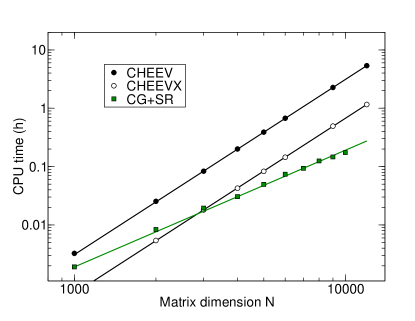
Figure 1: (Color online) CPU time on a single Opteron 275 core needed for the full diagonalization (CHEEV, black filled circles) or the computation of the 15 lowest eigenvalues of randomly filled Hermitian matrices, using the LAPACK library routine CHEEVX (black unfilled circles) or the CG+SR algorithm (green squares). The solid lines represent cubic (black) and quadratic fits (green) to the different data sets.

Often, not the DF itself but isolated exciton levels, especially bound states with pair excitation energies $E^{\Lambda}$ below the lowest QP gap, are of interest. Due to the limited spectral resolution and the possibility of vanishing oscillator strength, such excitations cannot be studied with the time-evolution method. The same holds for the analysis of excitonic wave functions, which requires the knowledge of the respective eigenvalues and eigenvectors. In those cases Eq. (3) needs to be solved directly, raising again the problem of excessive computational costs for complex systems. For Wannier-Mott-like excitonic states near the absorption edge, usually a fairly small BSE cutoff can be used in order to reduce the dimension of $\hat{H}$ Schleife et al. (2007). On the other hand, a large number of ${\bf k}$ points is required in the computations to ensure a sufficiently large crystal volume to accommodate the exciton, which can extend over several thousand unit cells according to exciton localization radii in the range of $10-100$ Å.

For excitons, numerical convergence is typically obtained for dimensions of $\hat{H}$ somewhere in the range of $N=10^{4}-10^{5}$. Direct matrix diagonalization schemes can be used at the lower end of the aforementioned range with computational times of a few CPU hours. However, due to the rapid $\mathcal{O}(N^{3})$ increase of computational costs, already problems of mid-range size are computationally too expensive for systematic studies.

Given the combination of a large-rank Hamiltonian and the interest in only a few of the smallest eigenvalues and corresponding eigenvectors renders the problem strongly reminiscent of the Kohn-Sham problem in DFT. Of course, this refers only to the dimensions of the problems, because in fact the BSE-EVP is less complicated, since no self-consistent update of the Hamiltonian is required. Using this observation, we propose to employ iterative minimization techniques similar to those used in DFT for the study of distinct exciton levels. These are based on the minimization of the Ritz functional,

$$\tilde{E}[\tilde{\phi}^{\Lambda}]=\frac{\langle\tilde{\phi}^{\Lambda}\,|\hat{H}|\,\tilde{\phi}^{\Lambda}\rangle}{\langle\tilde{\phi}^{\Lambda}|\tilde{\phi}^{\Lambda}\rangle},$$ (16)

with the trial vector $|\,\tilde{\phi}^{\Lambda}\rangle$. Obviously, an unconstrained minimization yields

$$\min_{\tilde{\phi}^{\Lambda}}\tilde{E}[\tilde{\phi}^{\Lambda}]=E^{\Lambda=1}=E[A^{\Lambda=1}],$$ (17)

the lowest (first) eigenvalue and the corresponding eigenvector of $\hat{H}$. For any higher eigenvalue $\Lambda>1$ the minimization needs to be constrained to the orthogonal complement of ${\rm span}(A^{1},\dots,A^{\Lambda-1})$. For the actual calculation we follow the scheme devised by Kalkreuter and Simma Kalkreuter and Simma (1996). There, consecutive conjugate gradient (CG) steps are performed together with intermediate diagonalizations of $\hat{H}$ in the low dimensional subspace ${\rm span}(\tilde{\phi}^{1},\dots,\tilde{\phi}^{n_{s}})$, so called subspace rotations (SR). The dimension $n_{s}$ of the subspace, thereby, roughly corresponds to the number of desired eigenvalues (typically $n_{s}\approx 20$). We have chosen a CG-based algorithm for the sake of simplicity and due to its robustness. Other algorithms, however, can be used as well and might also improve performance.

As already stressed above, in practice only a limited number of excitonic levels are of interest for the study of excitons. Further, this number does usually not depend on $N$, the dimension of $\hat{H}$. Therefore, under the assumption that the number of total CG steps is independent of $N$, the theoretical operation-count scaling of the CG+SR algorithm is found to be $\mathcal{O}(N^{2})$. The reason is that it involves only matrix-vector and vector-vector operations of dimension $N$ and diagonalizations of fixed-size $n_{s}\times n_{s}$ matrices. In general, the assumption of a constant number of total CG steps, is of course, not true, since it is determined by the convergence of the algorithm. However, it is found that the convergence depends little on the matrix dimension, but more on its conditioning. Figure 1 confirms that the CG+SR method scales basically like $\mathcal{O}(N^{2})$. The crossover point is found below $N=1000$ when competing with full diagonalization, or at 3000 when comparing against the LAPACK LAP CHEEVX routine for calculating selected eigenvalues and vectors of randomly filled Hermitian matrices.

Moreover, the CG+SR algorithm can be easily parallelized. MPI parallelization can help to meet the high memory demands for solving the BSE by utilizing distributed memory. However, also very reasonable speedups are obtained by using multiple processors.

II.5 Hybrid ${\bf k}$-point meshes

Figure 2: (Color online) The left panel illustrates the construction scheme for the hybrid ${\bf k}$-point meshes for a two-dimensional BZ. The ${\bf k}$ points of the coarse mesh are indicated by unfilled circles, those of the refined mesh by red dots. Further, the boundaries of the BZ and its inner part are indicated. Following the notation introduced in the text, the mesh shown here would be referred to as: hybrid $8:3:21.33$. The right panel shows the localization of the wave function for an 1$s$ Wannier-Mott exciton (with the parameters as in Sec. IV.1) in reciprocal space.

Even though the algorithm suggested in the preceding section keeps the computational costs for the calculation of excitons tractable, one drawback of the EVP remains – its extreme memory demands. Using very dense ${\bf k}$-point meshes the BSE Hamiltonian matrices (4) easily exceed 50 GB storage. Since the storage requirements scale quadratically with the number of ${\bf k}$ points, also the use of refined regular ${\bf k}$-point meshes rapidly approaches the limits of today’s supercomputers.

In order to reduce the memory demands, but also the computer time for setting up $\hat{H}$, one may benefit from noting that the wave functions of Wannier-Mott like excitons are well localized in ${\bf k}$ space (cf. Fig. 2). Therefore, it is reasonable to refine the ${\bf k}$ meshes only in the center of the BZ Rohlfing and Louie (1998a); Laskowski et al. (2005). Such a refinement, however, comes at the price of having to introduce varying weights (see Eqs. (9)–(11)), turning (3) into the generalized EVP (12).

The hybrid ${\bf k}$-point meshes used in this work are constructed in the following manner (see also Fig. 2). Firstly, the whole BZ is sampled using a comparably coarse mesh of Monkhorst-Pack ${\bf k}$ points Monkhorst and Pack (1976). Secondly, an inner region, fenced in by ${\bf k}$ points of the coarse mesh, is defined and the points inside this region including those on the borders are removed. In a third step, this inner region is filled with a fine-grained regular ${\bf k}$ mesh, which must be constructed accordingly to include ${\bf k}$ points on the borders of the inner region. Finally, the latter ${\bf k}$ points are centered inside their associated ${\bf k}$-space volume. In some cases it is meaningful to further refine the ${\bf k}$-point mesh in the inner region. This can be achieved by repeating steps two and three with respect to the inner mesh. Hereafter, meshes constructed accordingly by double repetition of the latter steps are referred to as double-hybrid ones.

The following notation is used to characterize the afore-described hybrid meshes (see also Fig. 2 and its caption). The first set of numbers indicates the ${\bf k}$ points in the outer (coarsely sampled) part of the BZ along the directions of the reciprocal basis. The second set indicates the size of the central part of the BZ (with refined sampling) with respect to the ${\bf k}$-point distance of the outer mesh, and the third set of numbers provides a measure for the sampling density inside the central part of the BZ. For better comparison the latter set corresponds to the number of regular ${\bf k}$ points in each direction necessary for sampling the whole BZ at the density achieved by the refined sampling. Double-hybrid meshes are characterized additionally by the size and sampling information of the second refinement region, encoded in the same manner as for the single hybrid meshes described before. To shorten the notation in case of isotropic sampling, only one number is given per set (see also the caption of Fig. 2).

One should note that the use of a hybrid mesh requires the knowledge of the dielectric screening $\epsilon^{-1}_{{\bf G}{\bf G}^{\prime}}({\bf q})$ at all vectors ${\bf q}={\bf k}-{\bf k}^{\prime}$ for the calculation of $W^{c}_{c^{\prime}}{}^{v}_{v^{\prime}}{}^{{\bf k}}_{{\bf k}^{\prime}}$ in (6). This also involves ${\bf q}$ points that are not part of the hybrid ${\bf k}$-point mesh, which is no concern in case of a constant or model screening as used throughout this work. However, if the screening is calculated in random-phase approximation (RPA), this constitutes an additional complication, that might be overcome by interpolating the screening for ${\bf q}$ points not included in the hybrid mesh.

III Computational Details

The results presented for MgO and InN in Sec. IV B and C are based on the results of ab initio DFT calculations, carried out using the Vienna Ab initio Simulation Package (VASP, Kresse and Furthmüller (1996); Shishkin and Kresse (2006)). The projector-augmented wave (PAW) method Blöchl (1994); Kresse and Joubert (1999) is used to model the electron-ion interaction. Plane waves up to a kinetic energy of 400 eV are included in the basis set of the electronic wave functions. Quasiparticle band structures are calculated for InN and MgO as a gauge by means of the HSE03+G₀W₀ approach with computational details as described in detail in Refs. Fuchs et al., 2007; Shishkin and Kresse, 2006. Within the explicit calculations the single-particle eigenvalues and wave functions are computed using exchange and correlation potentials according to the semi-empirical LDA+U (InN) or the GGA (MgO) scheme together with a scissors operator to correct for the gap underestimation. The BSE Hamiltonian is set up according to (4), whereby, the inverse dielectric function entering the screened interaction term $W^{c}_{c^{\prime}}{}^{v}_{v^{\prime}}{}^{{\bf k}}_{{\bf k}^{\prime}}$ is approximated by a ${\bf G}$-diagonal model function Bechstedt et al. (1992). The latter parametrically depends on the static electronic dielectric constant, which is taken from RPA calculations or experiment.

IV Results

In the following we present results obtained within the afore-introduced CG+SR approach for three applications. Firstly, we numerically study the two-band Wannier-Mott exciton in ${\bf k}$ space to demonstrate the applicability of the CG+SR approach and to extract some general trends. Further, the formation of excitons is studied for the large-gap material MgO and the narrow-gap semiconductor InN. Due to their band structures, the excitons occurring in both materials are expected to show Wannier-Mott-like character.

IV.1 The Wannier-Mott model

The probably most simplified model of a semiconductor band structure is the two-band model of two opposed parabolic bands, separated by the fundamental gap $E_{g}$. Within this model many fundamental properties can be calculated analytically, including the formation of a series of excitons below the absorption edge as found by Wannier Wannier (1937) and Mott Mott (1938). The analytic solution in three dimensions Elliott (1957) uses the fact that the BSE Hamiltonian (4) for the two-band model,

$$H^{c}_{c^{\prime}}{}^{v}_{v^{\prime}}{}^{{\bf k}}_{{\bf k}^{\prime}}=\delta_{cc^{\prime}}\delta_{vv^{\prime}}\,\left[\left(E_{g}+\frac{\hbar^{2}|{\bf k}|^{2}}{2\mu}\right)\delta_{{\bf k}{\bf k}^{\prime}}-\frac{4\pi e^{2}}{\Omega\epsilon_{0}|{\bf k}-{\bf k}^{\prime}|^{2}}\right],$$ (18)

resembles that of a hydrogen-like atom with the known solution of a Rydberg series for the discrete part of the spectrum,

$$E_{nlm}=E_{g}-R_{ex}/n^{2},$$ (19)

where the quantum numbers $n,\ l$, and $m$ of the hydrogen atom now label the excitonic states. Henceforth, $R_{ex}=R_{\infty}\mu/(m_{0}\epsilon_{0}^{2})$ denotes the excitonic Rydberg constant and $\epsilon_{0}$ determines the effective static and spatially constant screening of the Coulomb potential. The reduced mass $\mu=(m^{*-1}_{c}+m^{*-1}_{v})^{-1}$ follows from the effective masses of the valence and conduction band.

For the numerical solution the effective masses are chosen to be $1.0\ m_{0}$ and $0.5\ m_{0}$, such that $\mu=1/3\ m_{0}$. For the band gap a value of 3.0 eV is assumed. The calculations are performed in a simple cubic ${\bf k}$-space volume extending over $2\pi/3$ Å^-1, which naturally limits the maximum BSE cutoff to roughly 15.5 eV. Therefore, in the following only BSE-cutoff energies of 15 eV or below are considered. Using a screening constant of $\epsilon_{0}=4$, the excitonic Rydberg – corresponding to the highest possible exciton binding energy – amounts to $R_{ex}=283.45$ meV.

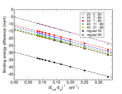
Figure 3: (Color online) Convergence of the binding energy of the 1$s$ exciton with the cutoff energy $E_{cut}$. Shown are the results for two regular (squares) and five hybrid ${\bf k}$-point meshes (circles and crosses). The hybrid meshes feature a common ${\bf k}$ density in the inner part, equivalent to that of the regular $80^{3}$ ${\bf k}$-point mesh. The $y$ axis refers to the difference of the numerically calculated binding energy and the analytical result of 283.45 meV. Solid lines indicate the results of linear fits inside the region 0.08–0.2 eV^-1. Dashed lines correspond to extrapolations based on these fits.

In order to treat (18) numerically in ${\bf k}$ space, it is necessary to introduce a ${\bf k}$-point sampling. Using Monkhorst-Pack meshes of regular ${\bf k}$ points, we first study the cutoff dependence of the binding energy of the 1$s$ ($n=1$, $l=0$) exciton. Figure 3 shows the results for two different regular meshes consisting of $40\!\times\!40\!\times\!40$ and $80\!\times\!80\!\times\!80$ points. According to Fig. 3 the 1$s$ binding energy increases with an increasing number of states included in $\hat{H}$ and a direct proportionality between the binding energy and $(E_{cut}-E_{g})^{-1}$ exists. While the latter relation cannot be expected to transfer to the situation of real semiconductors with a multitude of contributing bands, it is useful for estimating the effect of a limited BSE cutoff for the two-band model. Based upon linear extrapolation of the data between $E_{cut}=8-15$ eV (cf. Fig. 3), the 1$s$ binding energy at 15 eV cutoff is expected to underestimate the $E_{cut}\rightarrow\infty$ value by less than 5 meV, i.e. by less than 2%. The energy difference between the two ${\bf k}$-point sets is much larger, demanding for a better ${\bf k}$-point sampling.

Unfortunately, the $80\!\times\!80\!\times\!80$ ${\bf k}$-point Hamiltonian matrix at a cutoff of 10 eV already requires 95 GB RAM in single precision storage and would require 480 GB at $E_{cut}=15$ eV, due to the relation $E_{cut}\propto N^{2/3}$, specific for the two-band model. Therefore, the hybrid ${\bf k}$-point meshes introduced in Sec. II.5 are adopted in the following. The ${\bf k}$-point density in the central part of the BZ corresponds to $80\!\times\!80\!\times\!80$ ${\bf k}$ points in the full zone for all of them, thus allowing for a direct comparison to the results of the regular mesh with $80^{3}$ points. According to Fig. 3, it is possible to increase the distance of adjacent ${\bf k}$ points by a factor of two in the outer zone without introducing any significant error, if the inner zone extends to half of the BZ along each direction. Further, it should be noted that this $40:21:80$ mesh contains only about a fourth of the ${\bf k}$ points included in the regular $80^{3}$ mesh and thereby reduces the memory demands by a factor of 16. If the size of the densely sampled inner zone is reduced further, the binding energy increases. This is somehow unfortunate, because it counteracts the BSE-cutoff convergence. An analog trend is found, when the sampling in the outer region is reduced while the size and sampling density of the inner zone are kept fixed. Moreover, Fig. 3 shows that a trade-off between the minimum size of the inner zone and the sampling density of the outer zone exists, if one allows for a fixed error with respect to the corresponding regular mesh.

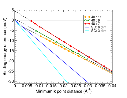
Figure 4: (Color online) Convergence of the $1s$ exciton binding energy with the ${\bf k}$-point sampling in the inner zone for three different sizes of the densely sampled inner zone and a fixed sampling density in the outer region of the BZ. The $y$ axis refers to the difference of the numerically calculated binding energy and the analytical result of 283.45 meV. The solid lines without symbols correspond to the singularity correction in the three-dimensional spherical approximation (Puschnig and Ambrosch-Draxl (2002), light blue) and the results from the six-dimensional integration (cf. (13), dark blue) as used in the present calculations.

Figure 4 shows the results for the $1s$ binding energy using ${\bf k}$ meshes with a fixed sampling density in the outer zone and a varying inner density and size of the inner zone. Obviously, the binding energy is directly proportional to the distance of adjacent ${\bf k}$ points, allowing for a linear extrapolation similar to the situation found for the convergence with the BSE cutoff. We would like to point out that the observed trend is not dominated by the singularity correction (cf. Eq. (13)), even though the latter obeys the same proportionality. This can be seen from Fig. 4, which also includes plots of the singularity correction for the three-dimensional spherical approximation Puschnig and Ambrosch-Draxl (2002) and the six-dimensional integration (13) as utilized in the present calculations. Taking into account that the binding energy and not the eigenvalue itself is plotted, it can be seen from Fig. 4 that the singularity correction already partially anticipates the ${\bf k}$-point convergence.

Figure 5: (Color online) Convergence of the first, second, and third shell ($n=1-3$) excitons with the ${\bf k}$-point sampling for two different sizes ($40:11$ - black lines with filled symbols and $40:7$ - red lines with unfilled symbols) of the densely sampled inner zone and a fixed sampling density in the outer region of the BZ. Different angular momentum quantum numbers $l$ are encoded by different symbols. Circles correspond to excitons with $s$, squares to $p$, triangles to $d$ character. The binding energy is given with respect to the analytical result of 283.45$/n^{2}$ meV with $n=1-3$.

Figure 5 shows the ${\bf k}$-point convergence of the first, second and third shell excitons for two sizes of the inner zone. In the realm of the two-band model all eigenvalues of a fixed principal quantum number $n$ are expected to be degenerate. Indeed, this degeneracy is found in the better-converged numerical results with a remaining error of about 0.1 meV or less. It is obvious from Fig. 5, that the rate of convergence might differ from one shell to another, but also within a shell of equal $n$, at least in the lower sampling regime. There also the linear behavior can be spoiled. This is readily understood, taking into account that the respective wave functions differ in their real-space localization. Therefore, since the exciton localization volume increases with the principal quantum number $n$, convergence with respect to the ${\bf k}$-point sampling is achieved harder for higher excitonic states. The same holds for excitons of lower quantum number $l$ when comparing them to others of the same shell $n$. Since these states become more localized in the reciprocal space, it is in principle possible to use hybrid meshes with an even smaller inner zone for computing the latter. This also becomes apparent from Fig. 5 comparing the different ${\bf k}$ meshes.

Figure 6: (Color online) Oscillator strengths of the $n=1-3$ excitons. Vertical and horizontal dashed lines indicate the analytical results for the exciton binding energies and oscillator strengths. Only excitons of angular momentum quantum number $l=0$ are found to be bright. All other excitons with $l>0$ are dipole-forbidden as indicated by vanishing oscillator strengths.

The oscillator strengths of the $n=1-3$ excitons are shown in Fig. 6. From the analytic description only excitons with $s$ character are expected to have non-vanishing oscillator strengths, which decay with increasing principal quantum number like $n^{-3}$. Indeed the numerical results follow these expectations with only small deviations. Further, the $l>0$ excitons are found to have vanishing oscillator strengths. This is in good agreement with the analytical result, predicting a direct proportionality between $f^{\Lambda}_{j}$ and the excitonic wave function at vanishing electron-hole distance in the case of ${\bf k}$-independent dipole-matrix elements (cf. Eq. (15)). Since hydrogenic wave functions are non-vanishing at $r=0$ only for $l=0$, the $l>0$ excitons are dipole-forbidden.

IV.2 MgO

Magnesium oxide (MgO) is a wide gap semiconductor with a gap of approximately 7.8 eV Roessler and Walker (1967). Up to very high pressures its equilibrium crystal structure is given by the rocksalt ($rs$) phase Schleife et al. (2006). In DFT-GGA the gap is strongly underestimated with a value of only 4.5 eV. Using first-order perturbation theory (G₀W₀) based on the DFT eigenvalues, the gap cannot be fully corrected, resulting in a GGA+G₀W₀ QP value of 6.8 eV. This deficiency can be mostly overcome starting from the nonlocal HSE03 XC functional. Together with perturbative QP corrections this approach results in a reliable electronic structure with a slightly underestimated gap of 7.5 eV. Other, even more sophisticated QP calculations, taking into account self-consistency van Schilfgaarde et al. (2006); Shishkin et al. (2007) or even vertex corrections Shishkin et al. (2007) in the self-energy, are found to overestimate the gap slightly by approximately the same amount. All of these schemes, however, share the drawback of being computationally by far too expensive to act as foundation for a study of bound excitons. Therefore, we use the GGA electronic structure as basis for the following studies, simply correcting the gap by a scissors shift of 2.98 eV. Figure 7 demonstrates that this approximation compares reasonably to the results of the more sophisticated HSE03+G₀W₀ approach. Especially the band dispersion is found to compare well between both approaches.

Figure 7: (Color online) MgO band structure in the GGA+$\Delta$ (solid black lines) and HSE03+G₀W₀ (red circles) approximation. The scissors shift $\Delta$ corrects for the gap underestimation.

Due to the rocksalt symmetry of the crystal lattice, MgO has an $s$-like conduction-band minimum (CBM) of $\Gamma_{1,c}$-type and a threefold-degenerate $p$-like valence-band maximum (VBM) of $\Gamma_{5,v}$-type. Two of the three uppermost valence bands show almost the same dispersion in the region around the $\Gamma$ point, while the third one is more dispersive. In this situation the formation of three degenerate, $s$-symmetric, excitons is expected from ${\bf k}\cdot{\bf p}$ theory Baldereschi and Lipari (1971). In the following we will label these excitons by A, B, and C. Indeed, for well converged ${\bf k}$-point samplings A, B, and C are found to be almost degenerate in our numerical calculations. The remaining splitting between (A, B) and C amounts to 0.30 meV, corresponding to less than 0.1% of the total binding energy, and might be due to numerical errors. In full agreement with the initial expectations all three excitons are visible in any polarization direction. For the screening in our calculations we use an electronic dielectric constant of $\epsilon_{\infty}=3.0$ which is in between the experimental value of 2.94 Martienssen and Warlimont (2005) and the value of 3.16 obtained in RPA Schleife et al. (2006). The influence of $\epsilon_{\infty}$ will be discussed below.

In the inset of Fig. 8 the convergence with respect to the BSE-cutoff energy is shown for the lowest three excitons. Clearly, the variation is not strictly linear as in the case of the two band model. However, at BSE-cutoff energies higher than 13 eV, corresponding to $(E_{cut}-E_{g})^{-1}=0.117$ eV^-1 the variation flattens out. Therefore, upon the data of Fig. 8, one can estimate that the exciton binding energies computed at a BSE-cutoff energy of 13.0 eV, as used in the following, are accurate within about 10 meV, i.e., less than 2.4% .

Figure 8: (Color online) Convergence of the MgO A, B (unfilled symbols), and C excitons (filled symbols) with respect to the ${\bf k}$-point sampling and the BSE-cutoff energy (inset). The cutoff convergence was studied using a regular mesh of $16\!\times\!16\!\times\!16$ ${\bf k}$ points, corresponding to a minimum ${\bf k}$-point distance of 0.16 Å^-1. Unfilled symbols refer to the binding energies of the A and B exciton, while filled symbols indicate those of the C exciton. The values of the hybrid mesh $10:7$ are extrapolated from the region of linear variation towards zero ${\bf k}$-point spacing.

The convergence with the number of ${\bf k}$ points for MgO is studied in Fig. 8. As found for the two-band model in the preceding section, we observe a linear variation with respect to the distance of neighboring ${\bf k}$ points. From this data an average binding energy for the A, B, and C excitons of 429 meV is derived by linear extrapolation. In comparison to experimental results of about 80 meV Roessler and Walker (1967) and 145 meV Whited et al. (1973) the calculated binding energies turn out to be drastically overestimated. This may be attributed to the neglect of dynamical screening Shindo (1970); Zimmermann (1971), which can influence the exciton binding energies significantly.

Since the experimental binding energies are of the order of the longitudinal optical phonon energies $\hbar\omega_{LO}=89$ meV Martienssen and Warlimont (2005), the lattice polarization can partially contribute to the screening of the electron-hole attraction. It is suggested Whited and Walker (1969); Zimmermann (1971); Bechstedt et al. (1980); Hahn et al. (2005a) that the static electronic dielectric constant $\epsilon_{\infty}$ has to be replaced by an effective dynamical one $\epsilon_{0}$, which is enlarged by parts of the lattice polarizability $\approx(\epsilon_{s}-\epsilon_{\infty})$. For MgO the effect of lattice polarization is very pronounced, as indicated by the large difference between the static electronic dielectric constant $\epsilon_{\infty}=3.0$ and the static dielectric constant $\epsilon_{s}=9.8$ Martienssen and Warlimont (2005). This may lead to a strong reduction of the binding between electron and hole. An estimate of the true effect would require an explicit treatment of the dynamical screening Shindo (1970); Zimmermann (1971), which is a computationally extremely demanding task. Therefore, we performed test calculations using an effective screening constant of $\epsilon_{0}=6.0$, as suggested from fits to the experimental exciton spectra Whited and Walker (1969), finding reduced exciton binding energies of in average 99.8 meV for the A, B, and C exciton.

It may be confusing to note that other theoretical studies Benedict et al. (1998); Wang et al. (2004) also predict much lower exciton binding energies closer to the experimental values, even though they use the static electronic dielectric constant or a RPA screened potential as well. We attribute most of the difference to the comparably coarse ${\bf k}$-point samplings of 256 Wang et al. (2004) and 1000 Benedict et al. (1998) ${\bf k}$ points in the full BZ used in these studies to calculate the dielectric function in an extended energy range. As demonstrated in Fig. 8 the exciton binding energies of MgO show a rather strong variation with the ${\bf k}$-point sampling density, leading to binding energies of 282 meV (A, B) and 191 meV (C) at a sampling density of 1000 ${\bf k}$ points in the BZ.

Figure 9: (Color online) Convergence of the second shell MgO excitons with respect to the ${\bf k}$-point sampling. Filled symbols refer to bright excitations, while the excitons marked by unfilled symbols have vanishing oscillator strength. The values of the double-hybrid mesh $10:5:34:7$ are extrapolated towards zero ${\bf k}$-point spacing. Further, the degeneracies of the different eigenvalue complexes are annotated.

An interesting effect of the real behavior of the electron-hole attraction can be observed for the higher pair excitation states. There, the non-spherical deviations of the potential $W$ from the model $|{\bf k}-{\bf k}^{\prime}|^{-2}$ dependence, are found to cause a splitting of the exciton levels 4–15 into five distinct levels. Three of the latter are threefold-degenerate, and one of them is found to contain the only three excitons with non-vanishing oscillator strength (cf. Fig. 9). Figure 9 shows the convergence of these states with respect to the distance of adjacent ${\bf k}$ points, whereby the linear variation at small ${\bf k}$-point distances indicates a reasonable convergence.

An open question is the absolute and relative influence of the LFEs or electron-hole exchange effects proportional to $\bar{v}$ in the pair Hamiltonian $\hat{H}$ (4) on the binding of the excitons. In order to study this effect, we setup the BSE Hamiltonian according to (4), once including both contributions ($W$ and $\bar{v}$) and with $W$ or $\bar{v}$ separately. Two ${\bf k}$-point samplings, given by the hybrid meshes $10:7:24$ and $10:7:20$, are used to account also for potentially different rates of convergence between the two contributions $W$ and $\bar{v}$. As expected, excitonic bound states cannot form in absence of the attractive screened Coulomb interaction $W$ between electron and hole. If, however, the electron-hole exchange $\bar{v}$ is suppressed, the binding energies of the lowest three excitons increase by about 58 meV. In relation to the exciton binding energy the reduction due to the LFEs amounts to about 14% or even more if dynamical screening is taken into account. The splitting of A, B, and C is slightly affected. From Table 1 it can be inferred, that the convergence rates of $W$ and $\bar{v}$ indeed differ. Actually, the contribution of $\bar{v}$ is found to be well converged at the probed ${\bf k}$-point sampling densities.

Hamiltonian	average A, B, C binding energy (meV)
	extrapolated	$10:7:24$	$10:7:20$
$\hat{H}=-W+2\bar{v}$	429.2	370.5	358.1
$\hat{H}=-W$	479.6	419.9	407.3

Table 1: Effect of the electron-hole exchange on the average exciton binding energy of the A, B, and C excitons in MgO.

IV.3 InN

Indium nitride (InN) is a narrow-gap semiconductor with a gap of approximately 0.6–0.7 eV Davydov et al. (2002); Matsuoka et al. (2002); Wu et al. (2002), crystallizing in the wurtzite (wz) structure under ambient conditions. Complications for the theoretical treatment of InN arise from the fact that DFT calculations including the In $4d$ electrons as valence states fail to predict a finite gap, no matter whether a local (LDA) or semilocal (GGA) approximation is used for the XC functional. Instead, the calculated band structures correspond to that of a zero-gap semiconductor with an, in comparison to the experiment, inverted ordering of the $\Gamma_{1,c}$ and $\Gamma_{5,v},\Gamma_{1,v}$ levels Furthmüller et al. (2005). It was shown recently Rinke et al. (2006); Fuchs et al. (2007) that these deficiencies can be overcome, using either the method of optimized effective potentials Rinke et al. (2006) or a hybrid XC functional like HSE03 Heyd et al. (2003). Both methods, however, are computationally too expensive for a study of excitons.

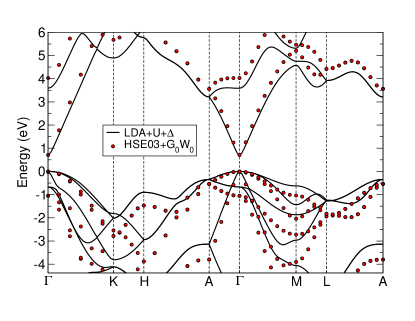
Figure 10: (Color online) InN band structure in the LDA+U+$\Delta$ (solid black lines) and HSE03+G₀W₀ (red circles) approximation. A U parameter of 3 eV is used for a good approximation of the HSE03+G₀W₀ band structure in the gap region. The scissors shift $\Delta$ corrects for the remaining gap underestimation.

Therefore, we retreat to the much simpler LDA+U scheme Anisimov et al. (1991, 1993); Franchini et al. (2005), trying to obtain a reasonable approximation of the HSE03+G₀W₀ band structure in the gap region around the $\Gamma$ point by tuning the intra-atomic Coulomb repulsion of the In $4d$ electrons by the U parameter. The band structure resulting from such an LDA+U calculation is shown in Fig. 10 in comparison to the QP band structure derived within the HSE03+G₀W₀ scheme. For clarity only the results fitting best, obtained for U=3 eV, are shown. Moreover, a scissors shift of 0.48 eV is used to open the gap additionally towards the value of 0.71 eV, as predicted by the HSE03+G₀W₀ calculations. Using the LDA+U approach, the effective masses at the $\Gamma$ point amount to approximately $2.2-2.5\ m_{0}$ for the uppermost valence bands ($v_{A},v_{B}$) of $\Gamma_{5,v}$ type. The masses of the crystal-field split off ($v_{C}$, $\Gamma_{1,v}$) and the first conduction band are much smaller with values of approximately $0.03\ m_{0}$. The respective values obtained from the HSE03 calculation differ notably, amounting to $0.9\ m_{0}$ for the mass of the $v_{A}$ and $v_{B}$ bands and $0.046\ m_{0}$ for the $v_{C}$ band and electron mass. We will try to assess the influence of the modified dispersion at the end of this section. The crystal-field splitting amounts to $\Delta_{cf}=$11.9 meV in the present approximation of LDA+U (U=3 eV), underestimating slightly the experimental values of $19-24$ meV Goldhahn et al. (2006) but also the HSE03+G₀W₀ value of 22.9 meV. We do not take into account the spin-orbit splitting of the valence bands, which amounts to 21.3 meV according to HSE03 calculations Fuchs et al. . For the static electronic dielectric constant $\epsilon_{\infty}$ entering $W$ a value of 7.9 is used. It corresponds to the average of the experimental values of the ordinary (7.83) Schley et al. (2007) and extraordinary (8.03) Goldhahn et al. (2004) polarization component determined from the analysis of the respective DF below the wz-InN gap of 0.68 eV.

Due to the wurtzite symmetry and the neglect of spin-orbit interaction, the VBM of InN is given by a twofold degenerate state. Therefore, the two strongest bound excitons (A, B), corresponding to the Wannier-Mott 1$s$ excitons, are expected to be twofold degenerate as well. A third 1$s$-like exciton (C) is expected to form between the first conduction and the crystal-field split-off $v_{C}$ band, at an eigenvalue differing from that of A and B by roughly $\Delta_{cf}$. Since optical transitions between $v_{A},v_{B}$ and the CBM at $\Gamma$ are dipole-allowed only in ordinary polarization (${\bf E}\perp{\bf c}$) and $v_{C}$-CBM transitions only in extraordinary polarization (${\bf E}\parallel{\bf c}$) Chuang and Chang (1996), the corresponding excitons are expected to have non-vanishing oscillator strengths in the respective directions Thomas and Hopfield (1959).

For a moment we limit ourselves to the discussion of the A and B excitons, which allow for a simple definition of their binding energies Laskowski et al. (2005). In agreement with the initial expectations A and B are found to be degenerate. The inset of Fig. 11 shows their convergence with respect to the BSE-cutoff energy. The overall variation of the binding energy with respect to the BSE cutoff is extremely weak, due to the very small binding energies and the strong localization of the lowest conduction band around the $\Gamma$ point (cf. Fig 10). According to Fig. 11, a BSE cutoff of 2 eV – as used in the following – should introduce an error of less than 0.1 meV.

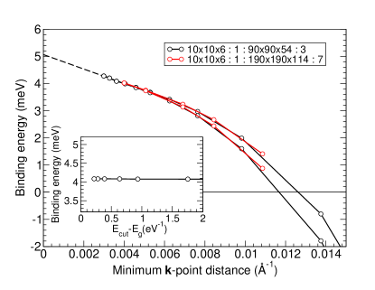
Figure 11: (Color online) Convergence of the InN A and B excitons with respect to the ${\bf k}$-point sampling and the BSE-cutoff energy (inset). The cutoff convergence was studied using the double hybrid ${\bf k}$-point mesh at a ${\bf k}$-point distance of 0.0036 Å^-1. The values of the double-hybrid meshes $10\!\times\!10\!\times\!6:1:90\!\times\!90\!\times\!54:1$ are extrapolated towards zero ${\bf k}$-point spacing.

The convergence with the number of ${\bf k}$ points is also demonstrated in Fig. 11. Due to the combination of a narrow gap, large screening, and a very small effective electron mass found for InN, extremely dense ${\bf k}$-point meshes are required to converge the exciton binding energies. Therefore, the double hybrid ${\bf k}$-point meshes, as introduced in Sec. II.5, are used to study the formation of excitonic states in InN. At the high-sampling limit of the studied ${\bf k}$-point meshes the linear variation with respect to the distance of adjacent ${\bf k}$ points, as observed for the two-band model and MgO, is restored. Extrapolating the binding energies of the lowest excitons towards zero ${\bf k}$-point distance, reveals binding energies of about 5.0 meV for the A and B exciton. The absolute difference between the computed values and the value of $6.5$ meV, estimated using the two-band model together with the appropriate masses and screening constant, is small.

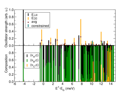
Figure 12: (Color online) Exciton spectrum of InN. The pair energies are given with respect to the lowest gap energy. The oscillator strengths are given in the upper panel. Black solid bars indicate the average oscillator strengths in ordinary polarization direction, while orange bars indicate the extraordinary polarization direction. The cyan bars indicate eigenstates of a pair Hamiltonian, which includes only contributions of the $v_{C}$ and the first conduction band. The red dots indicate the average oscillator strength. In the lower panel the contributions resulting from transitions between $v_{A},v_{B},v_{C}$ and the first conduction band c are analyzed (see text).

Figure 12 shows the exciton spectrum of InN together with the respective oscillator strengths for ordinary and extraordinary light polarization. Further, the contributions $c^{\Lambda}_{vc}=\sum_{{\bf k}}|\tilde{A}^{\Lambda}_{cv{\bf k}}|^{2}$ of the inter-band transitions between the 3 uppermost valence bands $v_{A}$, $v_{B}$, $v_{C}$ and the first conduction band $c$ have been analyzed. They are indicated by the relative lengths of the differently colored bars in the lower panel of Fig. 12. Obviously, as the respective contributions sum up to one, only the three single-particle pair states $(v_{A},c)$, $(v_{B},c)$, and $(v_{C},c)$ are found to contribute to the excitons in the energy interval shown in Fig. 12. Now, also the C exciton can be identified. To this end, we perform a constrained calculation with a pair Hamiltonian including only $(v_{C},c)$ transitions. The lowest eigenvalue of this Hamiltonian is found 2.3 meV below the $v_{C}$-CBM gap (cf. Fig. 12). Indeed, the unconstrained pair Hamiltonian gives rise to an eigenvalue at an only marginally higher energy, 2.1 meV below the $v_{C}$-CBM gap. The respective exciton, however, is found to be a nearly half-half mixture of $(v_{B},c)$ and $(v_{C},c)$ contributions. Further, it is clear from Fig. 12 that the latter exciton is neither the strongest bound state with contributions from $(v_{C},c)$ transitions, nor it is the first exciton visible in extra-ordinary polarization, nor it has the strongest oscillator strength in the latter polarization direction. Especially the latter two points are notable, since they contradict the initial expectations and may affect the experimental assignment of excitons. The reason for the observed behavior is found in the ${\bf k}$-point dependence of the single-particle optical oscillator strengths $\propto|\langle\varphi_{c{\bf k}}\,|p_{j}|\,\varphi_{v{\bf k}}\rangle|^{2}$. While the optical transitions $(v_{A},c)$ and $(v_{B},c)$ at $\Gamma$ are dipole-forbidden in extraordinary polarization, they are allowed and of comparable strength with the $(v_{C},c)$ transitions at off-$\Gamma$ ${\bf k}$ points.

Finally, we address the influence of the LDA+U approximation on the present results. The electron and $v_{C}$ effective masses at $\Gamma$ increase with increasing U, but underestimate the values calculated upon the HSE03 functional. Larger values than U=3 eV, however, yield a vanishing or even inverted crystal-field splitting – contradicting the HSE03 results and experimental findings. Due to the accompanying crossing and mixing of the $v_{A}$, $v_{B}$, and $v_{C}$ bands, values higher than U=3 eV are not meaningful starting points. The same holds for lower values of U, which predict much too small gaps and electron masses. The effect of the underestimated electron mass can be estimated within the two-band model, where the binding energy is found to depend linearly on the reduced effective mass. Therefore, the computed binding energies of the A and B excitons may underestimate the actual values by about 30%.

Apart from the influence of the U parameter the calculated exciton binding energies are influenced by the screening. Especially dynamical screening Shindo (1970); Zimmermann (1971) may reduce the exciton binding. The characteristic optical phonon energies ($\hbar\omega_{LO}=86$ meV Martienssen and Warlimont (2005)) are much larger than $R_{ex}$, so that the lattice polarization can fully contribute to the screening of the electron-hole attraction. For InN the static dielectric constant amounts to $\epsilon_{s}=13$ Davydov et al. (1999). Using $\epsilon_{s}$ for the screening instead of $\epsilon_{\infty}$ would significantly reduce the exciton binding energies to values below 2 meV. Consequently, Wannier-Mott excitons cannot be observed in the currently available InN samples, due to their high density of free carriers which is above the Mott-transition energy Davydov et al. (2002); Matsuoka et al. (2002); Wu et al. (2002).

V Summary and Conclusions

We have introduced a new and highly efficient numerical approach for the solution of the homogeneous BSE for bound electron-hole pair excitations in non-metals. The use of an iterative diagonalization scheme is demonstrated to diminish the computational costs for the calculation of bound electron-hole pair states significantly, allowing for the systematic study of excitonic Hamiltonians with ranks up to several hundred thousands. This is due to its, in comparison to the $\mathcal{O}(N^{3})$ scaling of direct diagonalization methods, favorable $\mathcal{O}(N^{2})$ scaling. Further, a hybrid ${\bf k}$-space sampling scheme is presented which allows a refined sampling in selected parts of the BZ and simultaneously avoids an artificial localization of the exciton wave functions. The corresponding discretization of the pair Hamiltonian EVP is performed and found to yield a generalized EVP with a diagonal overlap matrix.

As a first test and paradigmatic example the developed numerical approaches are applied to the Wannier-Mott exciton, which is solved numerically in the reciprocal space. Using realistic model parameters for the reduced effective mass and screening constant, the numerical convergence is systematically studied with special focus on the convergence with respect to the ${\bf k}$-point sampling. The well known analytical solution of a hydrogen-like exciton series is reproduced for the lowest bound pair states corresponding to the principle quantum numbers $n=1\dots 3$, including the expected degeneracies of exciton states and the oscillator strengths.

Further, the developed approaches are applied to the non-metallic materials MgO and InN, which both show Wannier-Mott-like excitons. The respective excitons, however, differ drastically in terms of their localization and consequently convergence, due to the very different electronic structures found for both materials. Nevertheless, the convergence trends identified for the Wannier-Mott model are found to hold and allow for the extrapolation of ${\bf k}$-point converged binding energies for the strongest bound excitons. If only the electronic screening is taken into account, the converged binding energies clearly exceed the experimental results. This is attributed to the influence of the lattice polarization on the screening and therewith the exciton binding.

Further, the achieved level of convergence, together with the account for the complete electronic structure, allows for the discussion of effects, which are not addressable in ${\bf k}\cdot{\bf p}$ theory. For InN, for instance, the often neglected ${\bf k}$-dependence of the single-particle oscillator strengths is shown to influence the polarization dependence of the lowest excitons drastically.

References

- Sham and Rice (1966) L. J. Sham and T. M. Rice, Phys. Rev. 144, 708 (1966).
- Hanke and Sham (1979) W. Hanke and L. J. Sham, Phys. Rev. Lett. 43, 387 (1979).
- Strinati (1988) G. Strinati, Rivista del Nuovo Cimento 11, 1 (1988).
- Onida et al. (2002) G. Onida, L. Reining, and A. Rubio, Rev. Mod. Phys. 74, 601 (2002).
- Hedin (1965) L. Hedin, Phys. Rev. 139, A796 (1965).
- Hybertsen and Louie (1985) M. S. Hybertsen and S. G. Louie, Phys. Rev. B 32, 7005 (1985).
- Godby et al. (1987) R. W. Godby, M. Schlüter, and L. J. Sham, Phys. Rev. B 35, 4170 (1987).
- Bechstedt (1992) F. Bechstedt, Adv. Solid State Phys. 32, 161 (1992).
- Aryasetiawan and Gunnarsson (1998) F. Aryasetiawan and O. Gunnarsson, Rep. Prog. Phys. 61, 237 (1998).
- Aulbur et al. (2000) W. G. Aulbur, L. Jönsson, and J. W. Wilkins, Solid State Physics: Advances in Research and Applications (Academic, San Diego, 2000), vol. 54, chap. Quasiparticle calculations in solids, p. 1.
- Albrecht et al. (1998) S. Albrecht, L. Reining, R. Del Sole, and G. Onida, Phys. Rev. Lett. 80, 4510 (1998).
- Rohlfing and Louie (1998a) M. Rohlfing and S. G. Louie, Phys. Rev. Lett. 81, 2312 (1998a).
- Benedict et al. (1998) L. X. Benedict, E. L. Shirley, and R. B. Bohn, Phys. Rev. Lett. 80, 4514 (1998).
- Schmidt et al. (2003) W. G. Schmidt, S. Glutsch, P. H. Hahn, and F. Bechstedt, Phys. Rev. B 67, 085307 (2003).
- Rohlfing and Louie (1999) M. Rohlfing and S. G. Louie, Phys. Rev. Lett. 83, 856 (1999).
- Hahn et al. (2002) P. H. Hahn, W. G. Schmidt, and F. Bechstedt, Phys. Rev. Lett. 88, 016402 (2002).
- Rohlfing and Louie (1998b) M. Rohlfing and S. G. Louie, Phys. Rev. Lett. 80, 3320 (1998b).
- Hahn et al. (2005a) P. H. Hahn, W. G. Schmidt, and F. Bechstedt, Phys. Rev. B 72, 245425 (2005a).
- Hahn et al. (2005b) P. H. Hahn, W. G. Schmidt, K. Seino, M. Preuss, F. Bechstedt, and J. Bernholc, Phys. Rev. Lett. 94, 037404 (2005b).
- Garbuio et al. (2006) V. Garbuio, M. Cascella, L. Reining, R. D. Sole, and O. Pulci, Phys. Rev. Lett. 97, 137402 (2006).
- Kittel (1996) C. Kittel, Introduction to Solid State Physics (John Wiley and Sons, New York, Chichester, 1996).
- Benedict and Shirley (1999) L. X. Benedict and E. L. Shirley, Phys. Rev. B 59, 5441 (1999).
- Bechstedt et al. (2005) F. Bechstedt, K. Seino, P. H. Hahn, and W. G. Schmidt, Phys. Rev. B 72, 245425 (2005).
- Hahn et al. (2005c) P. H. Hahn, K. Seino, W. G. Schmidt, J. Furthmüller, and F. Bechstedt, phys. stat. sol. (b) 242, 2720 (2005c).
- Yu and Cardona (1999) P. Y. Yu and M. Cardona, Fundamentals of Semiconductors (Springer-Verlag, Berlin, 1999).
- Elliott (1957) R. J. Elliott, Phys. Rev. B 108, 1384 (1957).
- Shinada and Sugano (1966) M. Shinada and S. Sugano, J. Phys. Soc. Japan 21, 1936 (1966).
- Rohlfing and Louie (2000) M. Rohlfing and S. G. Louie, Phys. Rev. B 62, 4927 (2000).
- Laskowski et al. (2005) R. Laskowski, N. E. Christensen, G. Santi, and C. Ambrosch-Draxl, Phys. Rev. B 72, 035204 (2005).
- Laskowski and Christensen (2006) R. Laskowski and N. E. Christensen, Phys. Rev. B 73, 045201 (2006).
- Denisov and Makarov (1973) M. Denisov and V. Makarov, phys. stat. sol. (b) 56, 9 (1973).
- Fu et al. (1999) H. Fu, L.-W. Wang, and A. Zunger, Phys. Rev. B 59, 5568 (1999).
- Rödl et al. (2008) C. Rödl, F. Fuchs, J. Furthmüller, and F. Bechstedt, Phys. Rev. B (2008), accepted.
- Anisimov et al. (1991) V. I. Anisimov, J. Zaanen, and O. K. Andersen, Phys. Rev. B 44, 943 (1991).
- Seidl et al. (1996) A. Seidl, A. Görling, P. Vogl, J. A. Majewski, and M. Levy, Phys. Rev. B 53, 3764 (1996).
- Fuchs et al. (2007) F. Fuchs, J. Furthmüller, F. Bechstedt, M. Shishkin, and G. Kresse, Phys. Rev. B 76, 115109 (2007).
- Puschnig and Ambrosch-Draxl (2002) P. Puschnig and C. Ambrosch-Draxl, Phys. Rev. B 66, 165105 (2002).
- Schleife et al. (2007) A. Schleife, C. Rödl, F. Fuchs, J. Furthmüller, and F. Bechstedt, Appl. Phys. Lett. 91, 241915 (2007).
- Kalkreuter and Simma (1996) T. Kalkreuter and H. Simma, Comput. Phys. Commun. 93, 33 (1996).
- (40) Linear Algebra PACKage, http://www.netlib.org/lapack/.
- Monkhorst and Pack (1976) H. J. Monkhorst and J. D. Pack, Phys. Rev. B 13, 5188 (1976).
- Kresse and Furthmüller (1996) G. Kresse and J. Furthmüller, Comp. Mat. Sci. 6, 15 (1996).
- Shishkin and Kresse (2006) M. Shishkin and G. Kresse, Phys. Rev. B 74, 035101 (2006).
- Blöchl (1994) P. E. Blöchl, Phys. Rev. B 50, 17953 (1994).
- Kresse and Joubert (1999) G. Kresse and D. Joubert, Phys. Rev. B 59, 1758 (1999).
- Bechstedt et al. (1992) F. Bechstedt, R. Del Sole, G. Cappellini, and L. Reining, Solid State Commun. 84, 765 (1992).
- Wannier (1937) G. H. Wannier, Phys. Rev. 52, 191 (1937).
- Mott (1938) N. F. Mott, Trans. Faraday Soc. 34, 500 (1938).
- Roessler and Walker (1967) D. M. Roessler and W. C. Walker, Phys. Rev. 159, 733 (1967).
- Schleife et al. (2006) A. Schleife, F. Fuchs, J. Furthmüller, and F. Bechstedt, Phys. Rev. B 73, 245212 (2006).
- van Schilfgaarde et al. (2006) M. van Schilfgaarde, T. Kotani, and S. Faleev, Phys. Rev. Lett. 96, 226402 (2006).
- Shishkin et al. (2007) M. Shishkin, M. Marsman, and G. Kresse, Phys. Rev. B 99, 246403 (2007).
- Baldereschi and Lipari (1971) A. Baldereschi and N. C. Lipari, Phys. Rev. B 3, 439 (1971).
- Martienssen and Warlimont (2005) W. Martienssen and H. Warlimont, eds., Springer Handbook of Condensed Matter and Materials Data (Springer-Verlag, Berlin, 2005), p. 660.
- Whited et al. (1973) R. C. Whited, C. J. Flaten, and W. C. Walker, Solid State Commun. 13, 1903 (1973).
- Shindo (1970) K. Shindo, J. Phys. Soc. Jpn. 29, 287 (1970).
- Zimmermann (1971) R. Zimmermann, phys. stat. sol. (b) 48, 603 (1971).
- Whited and Walker (1969) R. C. Whited and W. C. Walker, Phys. Rev. Lett. 22, 1428 (1969).
- Bechstedt et al. (1980) F. Bechstedt, R. Enderlein, and M. Koch, phys. stat. sol. (b) 99, 61 (1980).
- Wang et al. (2004) N. Wang, M. Rohlfing, P. Krüger, and J. Pollmann, Appl. Phys. A 78, 213 (2004).
- Davydov et al. (2002) V. Y. Davydov, A. A. Klochikhin, V. V. Emtsev, S. V. Ivanov, V. V. Vekshin, F. Bechstedt, J. Furthmüller, H. Harima, A. V. Mudryi, A. Hashimoto, et al., phys. stat. sol (b) p. 230 (2002).
- Matsuoka et al. (2002) T. Matsuoka, H. Okamoto, M. Nakao, H. Harima, and E. Kurimoto, Appl. Phys. Lett. 81, 1246 (2002).
- Wu et al. (2002) J. Wu, W. Walukiewicz, K. Yu, J. Ager III, E. Haller, H. Lu, W. J. Schaff, Y. Saito, and Y. Nanishi, Appl. Phys. Lett. 80, 3967 (2002).
- Furthmüller et al. (2005) J. Furthmüller, P. H. Hahn, F. Fuchs, and F. Bechstedt, Phys. Rev. B 72, 205106 (2005).
- Rinke et al. (2006) P. Rinke, M. Scheffler, A. Qteish, M. Winkelnkemper, and D. Bimberg, Appl. Phys. Lett. 89, 161919 (2006).
- Heyd et al. (2003) J. Heyd, G. E. Scuseria, and M. Ernzerhof, J. Chem. Phys. 118, 8207 (2003).
- Anisimov et al. (1993) V. I. Anisimov, I. V. Solovyev, M. A. Korotin, M. T. Czyżyk, and G. A. Sawatzky, Phys. Rev. B 48, 16929 (1993).
- Franchini et al. (2005) C. Franchini, V. Bayer, R. Podloucky, J. Paier, and G. Kresse, Phys. Rev. B 72, 045132 (2005).
- Goldhahn et al. (2006) R. Goldhahn, P. Schley, A. T. Winzer, M. Rakel, C. Cobet, N. Esser, H. Lu, and W. J. Schaff, J. Cryst. Growth 288, 273 (2006).
- (70) F. Fuchs, J. Furthmüller, and F. Bechstedt, unpublished.
- Schley et al. (2007) P. Schley, R. Goldhahn, A. T. Winzer, G. Gobsch, V. Cimalla, O. Ambacher, H. Lu, W. J. Schaff, M. Kurouchi, Y. Nanishi, et al., Phys. Rev. B 75, 205204 (2007).
- Goldhahn et al. (2004) R. Goldhahn, A. T. Winzer, V. Cimalla, O. Ambacher, C. Cobet, W. Richter, N. Esser, J. Furthmüller, F. Bechstedt, H. Lu, et al., Superlatt. Microstruct. 36, 591 (2004).
- Chuang and Chang (1996) S. L. Chuang and C. S. Chang, Phys. Rev. 54, 2491 (1996).
- Thomas and Hopfield (1959) D. G. Thomas and J. J. Hopfield, Phys. Rev. 116, 573 (1959).
- Davydov et al. (1999) V. Davydov, A. Klochikhin, M. Smirnov, V. Emtsev, V. Petrikov, I. Abroyan, A. Titov, I. Goncharuk, A. Smirnov, V. Mamutin, et al., phys. stat. sol. (b) 216, 779 (1999).