Photon-Mediated Interaction between Two Distant Atoms

Abstract

We study the photonic interactions between two distant atoms which are coupled by an optical element (a lens or an optical fiber) focussing part of their emitted radiation onto each other. Two regimes are distinguished depending on the ratio between the radiative lifetime of the atomic excited state and the propagation time of a photon between the two atoms. In the two regimes, well below saturation the dynamics exhibit either typical features of a bad resonator, where the atoms act as the mirrors, or typical characteristics of dipole-dipole interaction. We study the coherence properties of the emitted light and show that it carries signatures of the multiple scattering processes between the atoms. The model predictions are compared with the experimental results in J. Eschner et al., Nature 413, 495 (2001).

I Introduction

Control of photon-atom interaction lies at the heart of quantum technologies based on atomic and photonic systems ZollerRoadmap . Recent experiments demonstrated the quantum correlations between atoms and emitted photons Monroe04 ; Weinfurter06 ; Grangier06 . Atom-photon entanglement was then applied for entangling distant atoms by photon measurement Maunz . Further experiments demonstrated the possibility to spatially confine atoms with nanometric precision inside resonators Guthoerlein2001 ; Mundt ; Rauschenbeutel , and hence to control their coupling with the electromagnetic field modes of cavities. Such precision has permitted realizing quantum light sources with high degree of control Kimble04 ; Walther04 ; Kuhn2 ; Rempe07 ; Kimble08 , and hence to pose the basis for the realization of quantum networks based on atom-photon interfaces ZollerRoadmap .

Parallel to these experimental efforts, studies are also focussing on achieving strong coupling between atoms and photons by means of optical elements, such as lenses of large numerical aperture Eschner2001 ; Wilson ; Bushev2004 ; Sondermann07 ; Leuchs07 ; Kurtsiefer or optical fibers Spreeuw ; Balykin ; Arno . In particular, in Eschner2001 two distant atoms in front of a mirror were coupled by means of a lens, focussing the radiation emitted by one atom onto the other. In this setup, the first-order coherence was experimentally studied, showing an interference pattern when the optical path length between the atoms was varied. In earlier experiments with two trapped ions, far-field interference of their scattered light Itano , and their near-field interaction DeVoe were studied.

In this article we present an extensive theoretical study of the radiative properties of two distant atoms when they are coupled via an optical element, which could be an optical fiber or a lens, as sketched in Fig. 1. In this situation radiation is multiply scattered between the atoms, until it is finally dissipated into the external modes of the electromagnetic field. Our model is based on the theory developed in Alber ; Dorner for the case of a single atom interacting with itself via a mirror, and extends it to the situation of two coupled atoms. The theoretical predictions of our model reproduce the experimental results of Eschner2001 and allow us to identify possible measurements that highlight the multiple-scattering features. Moreover, the scattered photons are correlated with the scattering atoms, thereby establishing correlations and, in certain cases, entanglement between their internal excitations.

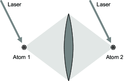
Figure 1: The dipolar transitions of two atoms, which are several optical wavelength apart, are coupled by a lens focussing part of their emitted radiation onto each other. In Eschner2001 a similar situation was realized, coupling two atoms via a mirror and a lens. Analogous dynamics can be observed when the atoms are trapped close to an optical fiber, see for instance Arno .

This article is organized as follows. In Sec. II we make some preliminary considerations on the system. In Sec. III we introduce the model in detail and solve the basic equations describing the coupled dynamics of the internal atomic states and few photons of the electromagnetic field. In Sec. IV we investigate in detail the radiative properties of the system, and in Sec. V we provide the details of the first- and second-order coherence of the light scattered by the atoms when they are weakly driven by a laser. In Sec. VI we provide some outlooks to the present work, and in the appendices we report details of the calculations.

II Preliminary considerations

The scattering cross section of an atomic dipole transition in free space is on the order of the square of its wavelength $\lambda$ Cohen-Tannoudji . Consequently, the free-space photonic interaction between two atomic dipoles at distance $d$ is determined by the ratio $\lambda/d$ Dipole-Dipole : when $d\ll\lambda$, strong modifications of the atomic emission spectrum of one atom due to the presence of another one are observable Dipole-Dipole ; DeVoe ; Savels07 ; when $d\gg\lambda$, these effects are negligible, and the atoms scatter photons independently. This behavior is dramatically modified if an optical system, like a lens with large numerical aperture or an optical fiber, focusses a significant fraction of the radiation emitted by one atom onto the other. This latter situation is sketched in Fig. 1 for the case of a lens that images the atoms onto each other.

When the photonic interaction between the atoms is mediated by an optical element, its strength is characterized by the fraction $\kappa$ of modes of the electromagnetic field which the optical system transforms into each other. Thus $\kappa$ replaces the scaling with $\lambda/d$ of the free-space case, and coupling over much larger distances than $\lambda$ may be achieved.

The atom-atom distance $d$, or more precisely the propagation time for a photon from one atom to the other via the optical element,

$$\tau=\frac{d}{c}$$ (1)

remains an important physical parameter of the photonic interaction, since it has to be compared with the radiative lifetime of the atomic dipolar transition $1/\gamma$, which determines the time scale on which the photonic excitation is dissipated into free space, as well as the length of the emitted photonic wave packet. When $\gamma\tau\gg 1$, the process of photon scattering by each atom is well localized in time and space: a photonic excitation is exchanged between the atoms at integer multiples of the delay time $\tau$, until its amplitude is damped to zero by emission into the external modes of the electromagnetic field. When $\gamma\tau\ll 1$, in contrast, multiple scattering events add up coherently during the excitation time of each atom, causing the spontaneous emission rate to be enhanced or suppressed, depending on the interatomic distance (modulo the wavelength). This regime is equivalent to dipole-dipole interaction with a delay time $\tau$.

In all cases, the system of two atoms confining radiation by multiple scattering shows some analogies with an optical resonator with low-reflectivity mirrors. This analogy is appropriate when the atomic transition is not saturated. Indeed, in this regime the radiative properties are very similar to those of a single atom interacting with itself via a mirror, studied in Eschner2001 ; Dorner ; Wilson . The peculiarity of the two-atom system becomes more evident when saturation effects are relevant. Some important properties, such as the creation of correlations and entanglement between the atoms via the multiply scattered photons, are identified when studying intensity-intensity correlation of the light scattered by the two-atom system, as discussed in Sec. V.

III The Model

In this section we develop the theoretical model for describing the dynamics of two atoms in presence of an optical element which focusses the radiation emitted by each atom into the other, as sketched in Fig. 1. In particular, we use the theoretical formalism in Dorner for one atom in front of a mirror, and generalize it to the case of two coupled atoms.

The system consists of two identical atoms of mass $M$, which are trapped at the positions ${\bf r_{1}}$ and ${\bf r_{2}}$, and whose relevant electronic degrees of freedom are the ground state $|g\rangle$ and the excited state $|e\rangle$ forming a dipole transition with dipole moment $D$, frequency $\omega_{0}$ and wavelength $\lambda=2\pi c/\omega_{0}$. The interatomic distance $d=|{\bf r_{2}}-{\bf r_{1}}|$ is such that $d\gg\lambda$, thus free-space dipole-dipole interaction between the atoms is negligible. We assume, however, that a lens (or an equivalent optical system) is placed between the atoms, which collects a fraction of the radiation from each atom and focusses it onto the other one. We use the plane wave decomposition for these modes and label them with $\rho$, in order to distinguish them from the external modes which do not couple the atoms; the latter are labeled with $\mu$, see also Fig. 2. The Hamiltonian of the system describes the interaction between the dipoles and the modes of the electromagnetic field, and can be decomposed into the sum

$$H=H_{0}+V_{\rm emf}\,,$$ (2)

where $H_{0}$ gives the self-energy and $V_{\rm emf}$ the interaction between the dipoles and the modes of the electromagnetic field. In detail,

$$H_{0}=\sum_{j=1,2}\hbar\omega_{0}\sigma^{+}_{j}\sigma^{-}_{j}+\sum_{\ell=\rho,\mu}\hbar\omega_{\ell}a_{\ell}^{\dagger}a_{\ell}\,,$$ (3)

where the first term describes the energy of the atoms, with $\sigma_{j}=|g\rangle_{j}\langle e|$ and $\sigma_{j}^{\dagger}$ its adjoint, and subscript $j=1,2$ labeling the atom. The second term is the free Hamiltonian of the transverse photon field where the summation runs over all field modes. We label by $\ell$ the mode with wave vector ${\bf k_{\ell}}$ and polarization $\mbox{\boldmath$\epsilon$}_{\ell}\perp{\bf k_{\ell}}$, while $a_{\ell}^{\dagger}$ and $a_{\ell}$ are the creation and annihilation operators for a photon in that mode, obeying the commutation relation $\left[a_{\ell},a_{\ell^{\prime}}^{\dagger}\right]=\delta_{\ell,\ell^{\prime}}$. In particular, the modes with label $\ell=\rho$ are the ones which couple the atoms via the lens.

The interaction of the atoms with the electromagnetic field, $V_{\rm emf}$, is given in the electric dipole and rotating wave approximation, and takes the form

$$V_{\rm emf} = -{\rm i}\hbar\sum_{j=1,2}\sigma_{j}^{+}\sum_{\ell=\rho,\mu}g_{\ell}a_{\ell}{\rm e}^{{\rm i}{\bf k_{\ell}}\cdot{\bf r_{j}}}+{\rm H.c.}\,,$$ (4)

where

$$g_{\ell}=\left(\mbox{\boldmath$D$}\cdot\mbox{\boldmath$\epsilon$}_{\ell}\right)\sqrt{\omega_{\ell}/(2\varepsilon_{0}\hbar{\mathcal{V}})}$$

with the vacuum electric permittivity $\varepsilon_{0}$ and the quantization volume $\mathcal{V}$.

In presence of a laser driving the atoms the Hamiltonian will be given by

$$H^{\prime}=H+V_{L}(t)\,,$$ (5)

where the term $V_{L}$ describes the atom-laser coupling and reads

$$V_{L}=\hbar\Omega\sum_{j=1,2}\sigma^{+}_{j}{\rm e}^{{\rm i}({\bf k_{L}}\cdot{\bf r_{j}}-\omega_{L}t)}+{\rm H.c.}$$ (6)

Here, the laser is a classical field at frequency $\omega_{L}$ Cohen-Tannoudji , $\Omega$ is the coupling strength, and ${\bf k_{L}}$ is the wave vector of the incident laser beam.

The dynamics of the system is studied by solving the Schrödinger equation treating the interaction of the atoms with the electromagnetic field as a perturbation. For this purpose, the wave function $|\psi(t)\rangle$ of the atoms and the field at time $t$, in the interaction picture with respect to $H_{0}$, is described by

$$|\psi(t)\rangle=b_{e}^{(1)}(t)|e_{1},g_{2},0\rangle+b_{e}^{(2)}(t)|g_{1},e_{2},0\rangle$$ (7)

$$+\sum_{\rho}b_{g}^{(\rho)}(t)|g_{1},g_{2},1_{\rho},0_{\mu}\rangle+\sum_{\mu}b_{g}^{(\mu)}(t)|g_{1},g_{2},0_{\rho},1_{\mu}\rangle\,,$$

where the state $|0\rangle$ corresponds to the vacuum state of the electromagnetic field, and the state $|n_{\mu}\rangle$ ($|n_{\rho}\rangle$) to $n$ photons in mode $\mu$ ($\rho$). In Eq. (7) we have assumed that at most one excitation is present in the system. In particular, the coefficients $b_{e}^{(j)}(t)$ are the probability amplitudes at time $t$ for atom $j$ being in the excited state, while the coefficient $b_{g}^{(\ell)}(t)$ gives the probability amplitude to find a photon in the field mode $\ell$ at time $t$, with both atoms in the ground state. For later convenience, we also introduce the probability amplitudes $b_{g}^{(j,\ell)}(t)$, with

$$b_{g}^{(\ell)}(t)=b_{g}^{(1,\ell)}(t)+b_{g}^{(2,\ell)}(t)\,,$$

and which distinguish which atom has emitted the photon into mode $\ell$.

We will solve the Schrödinger equation using this ansatz first in absence and then in presence of a laser driving the atoms. In particular, we will study the dynamics as a function of two important physical quantities which characterize the system. The first is the time delay $\tau$ for light to propagate from one atom to the other, defined in Eq. (1). As noted before, we consider the case $c\tau\gg\lambda$. The second important quantity is the strength of the photonic coupling between the atoms mediated by the lens, which is defined through the fraction of $4\pi$ solid angle within which the radiation from one atom is focussed onto the other. This corresponds to the fraction of modes labeled with $\rho$, which propagate from one atom to the other via the lens. We denote the coupling by the dimensionless parameter $\kappa$,

$$\kappa = \sum_{\bf n_{\rho}}\left(1-|{\bf D}\cdot{\bf n_{\rho}}|^{2}/|{\bf D}|^{2}\right)$$ (8)

$$= \frac{3}{8\pi}\int_{\delta\Omega}d\Omega_{0}\left(1-|{\bf D}\cdot{\bf n}|^{2}/|{\bf D}|^{2}\right)\,,$$

where ${\bf n_{\rho}}={\bf k_{\rho}}/k$ and $\delta\Omega$ is the solid angle collected by the lens. The value of $\kappa$ lies in the interval $0<\kappa<1$, whereby $\kappa\to 0$ corresponds to the limit without the lens and $\kappa\to 1$ would describe an ideal optical system that maps all radiation from one atom onto the other.

III.1 Perturbative solution of the Schrödinger equation in absence of the laser.

When the atom-laser coupling is set to zero, then in the reference frame of the atoms the coefficients $b_{e}^{(j)},b_{g}^{(j,\rho)},b_{g}^{(j,\mu)}$ obey the differential equations

$$\dot{b}_{e}^{(j)}(t) = -\sum_{\rho}g_{\rho}{\rm e}^{{\rm i}{\bf k_{\rho}}\cdot{\bf r_{j}}}{\rm e}^{{\rm i}(\omega_{0}-\omega_{\rho})t}b_{g}^{(\rho)}(t)$$ (9a)

$$-\sum_{\mu}g_{\mu}{\rm e}^{{\rm i}{\bf k_{\mu}}\cdot{\bf r_{j}}}{\rm e}^{{\rm i}(\omega_{0}-\omega_{\mu})t}b_{g}^{(j,\mu)}(t)\,,$$

$$\dot{b}_{g}^{(j,\rho)}(t) = \,g_{\rho}{\rm e}^{-{\rm i}{\bf k_{\rho}}\cdot{\bf r_{j}}}{\rm e}^{-{\rm i}(\omega_{0}-\omega_{\rho})t}b_{e}^{(j)}(t)\,,$$ (9b)

$$\dot{b}_{g}^{(j,\mu)}(t) = \,\,g_{\mu}{\rm e}^{-{\rm i}{\bf k_{\mu}}\cdot{\bf r_{j}}}{\rm e}^{-{\rm i}(\omega_{0}-\omega_{\mu})t}b_{e}^{(j)}(t)\,,$$ (9c)

where in the regime $|{\bf r_{2}}-{\bf r_{1}}|\gg\lambda$ we have neglected processes in which a photon emitted into a mode $\mu$ by one atom is reabsorbed by the other one.

A closed form for the coefficients of the dipole excitations is found by summing over the modes of the electromagnetic field and by applying the Wigner-Weisskopf approximation as in Dorner . The details of the calculation are reported in App. A. The resulting equations take the form

$$\dot{b}_{e}^{(1)}(t) = -\frac{\gamma}{2}b_{e}^{(1)}(t)-\kappa\frac{\gamma}{2}e^{{\rm i}\omega_{0}\tau}b_{e}^{(2)}(t-\tau)\Theta(t-\tau)\,,$$

$$\dot{b}_{e}^{(2)}(t) = -\frac{\gamma}{2}b_{e}^{(2)}(t)-\kappa\frac{\gamma}{2}e^{{\rm i}\omega_{0}\tau}b_{e}^{(1)}(t-\tau)\Theta(t-\tau).$$

Equations (LABEL:eqn:b1)-(LABEL:eqn:b2) show different behaviour depending on whether $t\leq\tau$ or $t>\tau$. For $t\leq\tau$ these equations are decoupled and describe exponential damping at rate $\gamma$ of the single-atom excited-state occupation, as in free space. After the time $\tau$, the coupling by light scattering from each atom onto the other appears, its strength being set by the parameter $\kappa$.

We proceed by solving Eqs. (LABEL:eqn:b1)-(LABEL:eqn:b2) for an arbitrary initial state with a single atomic excitation,

$$|\psi(0)\rangle=\alpha_{1}|e,g,0\rangle+\alpha_{2}|g,e,0\rangle\,.$$ (11)

A simple solution is then found by using the decomposition into symmetric and antisymmetric coefficients $C_{\pm}(t)$,

$$b_{e}^{(1)}(t)=(C_{+}(t)+C_{-}(t))/2\,,$$ (12)

$$b_{e}^{(2)}(t)=(C_{+}(t)-C_{-}(t))/2\,,$$ (13)

obeying the differential equations

$$\dot{C}_{\pm}(t)=-\frac{\gamma}{2}C_{\pm}(t)\mp\kappa\frac{\gamma}{2}{\rm e}^{{\rm i}\omega_{0}\tau}C_{\pm}(t-\tau)\Theta(t-\tau)\,,$$ (14)

whose solution is Dung

$$C_{\pm}(t)=C_{\pm}(0)\sum_{k=0}^{\infty}(\pm 1)^{k}I_{k}(t),$$

with

$$I_{k}(t)=\frac{(-\kappa\frac{\gamma}{2}{\rm e}^{{\rm i}\omega_{0}\tau})^{k}}{k!}(t-k\tau)^{k}e^{-\frac{\gamma}{2}(t-k\tau)}\Theta(t-k\tau)\,.$$ (15)

Correspondingly, the probability amplitudes for the excited states are

$$b_{e}^{(1)}(t) = \alpha_{1}\sum_{k}I_{2k}(t)+\alpha_{2}\sum_{k}I_{2k+1}(t)\,,$$ (16a)

$$b_{e}^{(2)}(t) = \alpha_{1}\sum_{k}I_{2k+1}(t)+\alpha_{2}\sum_{k}I_{2k}(t)\,,$$ (16b)

while the probability amplitudes $b_{g}^{(j,\mu)}(t)$ for the emission of a photon into mode $\mu$ by atom $j$ are given by

$$b_{g}^{(1,\mu)}(t) = \frac{g_{\mu}{\rm e}^{-{\rm i}{\bf k_{\mu}}\cdot{\bf r_{1}}}}{\frac{\gamma}{2}+{\rm i}\delta_{\mu}}\,,$$

$$\times\sum_{k=0}^{\infty}\left[\alpha_{1}H_{2k}(t,\omega_{\mu})+\alpha_{2}H_{2k+1}(t,\omega_{\mu})\right]$$

$$b_{g}^{(2,\mu)}(t) = \frac{g_{\mu}{\rm e}^{-{\rm i}{\bf k_{\mu}}\cdot{\bf r_{2}}}}{\frac{\gamma}{2}+{\rm i}\delta_{\mu}}$$

$$\times\sum_{k=0}^{\infty}\left[\alpha_{1}H_{2k+1}(t,\omega_{\mu})+\alpha_{2}H_{2k}(t,\omega_{\mu})\right]\,,$$

with

$$\delta_{\mu}=\omega_{0}-\omega_{\mu}\,.$$ (19)

In Eqs. (III.1)-(III.1) we assumed that the electromagnetic field is initially in the vacuum state, $b_{g}^{\mu}(0)=0$, and we introduced the function

$$H_{k}(t,\omega)=\frac{(-\kappa\frac{\gamma}{2}{\rm e}^{{\rm i}\omega\tau})^{k}}{k!}(t_{k})^{k}G_{k}\left[({\rm i}\delta_{\mu}+\gamma/2)t_{k}\right]\Theta(t_{k})\,,$$

(20)

with $t_{k}=t-k\tau$ and

$$G_{k}(s)=~{}{{}_{1}}F_{1}(k,k+1,-s)-e^{-s}\,,$$ (21)

where ${}_{1}F_{1}(k,k+1,-s)$ is the confluent hypergeometric function Abramowitz . In the limit $\kappa\rightarrow 0$, i.e. when there is no coupling between the atoms, Eqs. (III.1)-(III.1) reduce to the usual free space decay spectrum of two independent dipoles with linewidth $\gamma$ Heitler .

III.2 Perturbative solution of the Schrödinger equation in presence of the laser.

We consider now the situation that the atoms are weakly driven by a laser at intensity $\Omega$. Hence, we set $\Omega\neq 0$ in the Schrödinger equation and solve the dynamics of the new Hamiltonian assuming that $V_{L}$ is a weak perturbation to the atomic dynamics. We use the ansatz for the wave function in Eq. (7), where we denote now the probability amplitudes by $b_{e}^{(j)}(t),b_{g}^{(j,\ell)}(t),b_{g}^{(\ell)}(t)\to c_{e}^{(j)}(t),c_{g}^{(j,\ell)}(t),c_{g}^{(\ell)}(t)$ (with $j=1,2$ and $\ell=\mu,\rho$). Let $|\psi(0)\rangle=|g_{1},g_{2},0\rangle$ be the initial state. By solving the coupled differential equations for the probability amplitudes in first order in $\Omega$ and in the reference frame rotating at the laser frequency $\omega_{L}$ we find

$$c_{e}^{(1)}(t) = -{\rm i}/\hbar\int_{0}^{t}{\rm d}t^{\prime}{\rm e}^{{\rm i}\omega_{L}t}\langle e_{1},g_{2},0|{\rm e}^{-{\rm i}H(t-t^{\prime})/\hbar}V_{L}(t^{\prime}){\rm e}^{-{\rm i}Ht^{\prime}/\hbar}|g_{1},g_{2},0\rangle$$ (22)

$$= -{\rm i}\sqrt{2}\Omega\int_{0}^{t}{\rm d}t^{\prime}{\rm e}^{{\rm i}\omega_{L}(t-t^{\prime})}\langle e_{1},g_{2},0|\left[{\rm e}^{-{\rm i}H(t-t^{\prime})/\hbar}\left({\rm e}^{{\rm i}{\bf k_{L}}\cdot{\bf r_{1}}}|e_{1},g_{2},0\rangle+{\rm e}^{{\rm i}{\bf k_{L}}\cdot{\bf r_{2}}}|g_{1},e_{2},0\rangle\right)/\sqrt{2}\right]\,.$$

Corresponding expressions are derived for $c_{e}^{(2)}(t)$ and $c_{g}^{(j)}(t)$. The term inside the square bracket corresponds to the time evolution of the state $|\beta_{0}\rangle=({\rm e}^{{\rm i}{\bf k_{L}}\cdot{\bf r_{1}}}|e_{1},g_{2},0\rangle+{\rm e}^{{\rm i}{\bf k_{L}}\cdot{\bf r_{2}}}|g_{1},e_{2},0\rangle)/\sqrt{2}$ when there is no laser. Hence we can write

$$c_{e}^{(j)}(t)=-{\rm i}\sqrt{2}\Omega\int_{0}^{t}{\rm d}t^{\prime}{\rm e}^{{\rm i}\Delta t^{\prime}}b_{e}^{(j)}(t^{\prime})\,,$$ (23a)

$$c_{g}^{{(\ell)}}(t)=-{\rm i}\sqrt{2}\Omega\int_{0}^{t}{\rm d}t^{\prime}{\rm e}^{-{\rm i}\Delta_{\ell}t^{\prime}}b_{g}^{(\ell)}(t^{\prime})\,,$$ (23b)

where $\ell=\rho,\mu$ and we have introduced the detunings

$$\Delta = \omega_{0}-\omega_{L}\,,$$ (24a)

$$\Delta_{\ell} = \omega_{\ell}-\omega_{L}\,.$$ (24b)

The coefficients $b_{e}^{(j)}$ and $b_{g}^{(\mu)}$ are found using the solutions derived in Sec. III.1 when the initial state is $|\beta_{0}\rangle$. One gets

$$c_{e}^{(1)}(t) = \frac{-{\rm i}\Omega}{\frac{\gamma}{2}+{\rm i}\Delta}{\rm e}^{{\rm i}{\bf k_{L}}\cdot{\bf r_{1}}}$$

$$\times \sum_{k=0}^{\infty}\left[H_{2k}(t,\omega_{L})+{\rm e}^{{\rm i}\varphi_{L}}H_{2k+1}(t,\omega_{L})\right]\,,$$

with

$$\varphi_{L}={\bf k_{L}}\cdot({\bf r_{2}}-{\bf r_{1}})\,.$$ (26)

The equation for $c_{e}^{(2)}(t)$ results from Eq. (III.2) by interchanging the indices $1\leftrightarrow 2$. The probability amplitudes $c_{g}^{(j,\mu)}(t)$ are found using Eq. (III.1) in Eq. (23b), assuming that initially both atoms are in the ground state and the electromagnetic field in the vacuum state. One gets

$$c_{g}^{(1,\mu)}(t)=-{\rm i}\frac{\Omega g_{\mu}}{\frac{\gamma}{2}+{\rm i}\delta_{\mu}}\int_{0}^{t}{\rm d}t^{\prime}{\rm e}^{{\rm i}(\omega_{L}-\omega_{\mu})t^{\prime}}{\rm e}^{{\rm i}({\bf k_{L}}-{\bf k}_{\mu})\cdot{\bf r_{1}}}$$

$$\times\sum_{k=0}^{\infty}\left[H_{2k}(t^{\prime},\omega_{\mu})+{\rm e}^{{\rm i}\varphi_{L}}H_{2k+1}(t^{\prime},\omega_{\mu})\right]\,,$$ (27)

with $\delta_{\mu}$ given in Eq. (19). The probability amplitude $c_{g}^{(2,\mu)}(t)$ for atom 2 is obtained by swapping the superscripts $1\leftrightarrow 2$ in Eq. (27).

III.3 Discussion

The probability amplitudes of the atomic excited states in absence and in presence of the laser, given in Eqs. (16) and (III.2), respectively, are the coherent sums over contributions starting at different instants of time $\tau_{k}=t-k\tau$. These contributions correspond to the effect of $k$ exchanges of a photonic excitation between the two atoms. In particular, for the case of atom 1, the contributions at $\tau_{2k}$ correspond to an excitation which propagated to atom 2 and back. Hence, in Eq. (16) this term vanishes when initially only atom 2 is excited. Similarly, the contributions at $t=\tau_{2k+1}$ vanish when atom 2 is initially in the ground state. Similar considerations apply for the case in which the laser drives the atom, Eq. (III.2).

An important property of these equations is that each term of the sum has a well-defined phase, which is an integer multiple of $\omega_{0}\tau$ ($\omega_{L}\tau$ with the laser excitation). At the same time the contributions are damped by an exponential function at rate $\gamma$. Consequently, the individual terms show interference if over the time $\tau$ they do not decay appreciably. This shows in more detail how the radiative properties of the system are determined by the parameter $\gamma\tau$, the ratio between the delay time and the excited state lifetime. In particular, for $\gamma\tau\gg 1$ interference plays no role, and the photonic excitation is a wave packet bouncing between the two atoms, until its intensity is damped to zero by scattering into free space. For $\gamma\tau\ll 1$ the terms in (15) add up coherently and interfere. The effect of the interaction hence modifies the radiative properties of the atoms, and the dynamics are analogous to an effective dipole-dipole interaction Dipole-Dipole .

In this perspective, the optical set-up composed by two atoms and the lens can be considered like a resonator, where the atoms are mirrors of low reflectivity and reflection bandwidth $\gamma/2$, while $2\tau$ is the round-trip time. The parameter $\gamma\tau$ hence gives the number of modes that this peculiar ”two-atom cavity” sustains: for $\gamma\tau\gg 1$ it sustains several modes and can be considered a ”multi-mode resonator”. Conversely, for $\gamma\tau\ll 1$ only a single mode of radiation is supported, and we will denote this case as ”single-mode resonator”.

Using this insight, we now analyze the probability amplitude and the spectrum of the emitted photons in the external modes labeled with $\mu$. Let us first assume that the laser is absent, and that initially atom 1 is in the excited state, i.e. $\alpha_{1}=1,\alpha_{2}=0$ in Eq. (11). From Eqs. (III.1)-(III.1), the amplitude probability for the state of the field reads

$$b_{g}^{(\mu)}(t) = \frac{g_{\mu}}{\frac{\gamma}{2}+{\rm i}\delta_{\mu}}\sum_{k=0}^{\infty}$$

$$\times\Bigl{[}{\rm e}^{-{\rm i}{\bf k_{\mu}}\cdot{\bf r_{1}}}H_{2k}(t,\omega_{\mu})+{\rm e}^{-{\rm i}{\bf k_{\mu}}\cdot{\bf r_{2}}}H_{2k+1}(t,\omega_{\mu})\Bigr{]}$$

where the two terms under the sum account for the respective contributions of the two atoms to the emission into the field mode. The label $k$ gives the number of photon exchanges between the two atoms before the photon is finally emitted into the external mode $\mu$.

In the long time limit Eq. (III.3) reduces to the form

$$b_{g}^{(\mu)}(t\to\infty)=g_{\mu}{\rm e}^{-{\rm i}{\bf k_{\mu}}\cdot{\bf r_{1}}}\frac{(\frac{\gamma}{2}+{\rm i}\delta_{\mu})-\kappa\frac{\gamma}{2}{\rm e}^{{\rm i}\omega_{\mu}\tau(1+\cos\vartheta)}}{(\frac{\gamma}{2}+{\rm i}\delta_{\mu})^{2}-(\kappa\frac{\gamma}{2}{\rm e}^{{\rm i}\omega_{\mu}\tau})^{2}}\,,$$

where $\vartheta$ denotes the angle between the vector ${\bf r_{1}}-{\bf r_{2}}$ and the wave vector ${\bf k_{\mu}}$ of the mode, see Fig. 2. At $\vartheta=\pi/2$, in particular, the probability to measure a photon in mode $\mu$ is given by

$$|b_{g}^{(\mu)}(t\to\infty)|^{2}=\frac{g_{\mu}^{2}}{\frac{\gamma^{2}}{4}[1+\kappa\cos\omega_{\mu}\tau]^{2}+[\omega_{0}-\omega_{\mu}+\kappa\frac{\gamma}{2}\sin\omega_{\mu}\tau]^{2}}$$ (29)

showing that the spectrum exhibits a modulation at multiples of the frequency $1/2\tau$. In the resonator picture, the modulation peaks are at the mode frequencies of the resonator, and $1/2\tau$ corresponds to the free spectral range. The spectral modulation will be visible when $\gamma\tau\gg 1$, i.e. when the system is in the ”multi-mode-resonator” regime. On the other hand, in the ”single-mode” regime $\gamma\tau\ll 1$, one will observe a change of the radiative linewidth, which depends on the phase $\omega_{0}\tau$.

When the atoms are laser-driven, the probability amplitude for the excited state occupation in the long-time limit is

$$c_{e}^{(1)}(t\to\infty) = \frac{-{\rm i}\Omega}{\frac{\gamma}{2}+{\rm i}\Delta}{\rm e}^{{\rm i}{\bf k_{L}}\cdot{\bf r_{1}}}\left(\frac{1-K{\rm e}^{{\rm i}\varphi_{L}}}{1-K^{2}}\right)\,,$$ (30)

while the probability amplitude that mode $\mu$ is occupied by one photon scattered by atom 1 takes the form

$$c_{g}^{(1,\mu)}(t) = 2\pi\delta^{(t)}(\Delta_{\mu})\frac{g_{\mu}\Omega{\rm e}^{-{\rm i}\Delta_{\mu}t/2}}{({\rm i}\frac{\gamma}{2}-\delta_{\mu})(1-K^{2})}$$ (31)

$$\times {\rm e}^{{\rm i}({\bf k_{L}}-{\bf k_{\mu}})\cdot{\bf r_{1}}}\left(1-K{\rm e}^{{\rm i}\varphi_{L}}\right)+{\rm O}(1)~{}~{}.$$

Here

$$K=\kappa\frac{\gamma}{2}\frac{{\rm e}^{{\rm i}\omega_{L}\tau}}{\frac{\gamma}{2}+{\rm i}\Delta}$$ (32)

and $\delta^{(t)}(\Delta)=\frac{1}{\pi}\frac{\sin(\Delta t/2)}{\Delta}$ is the diffraction function Cohen-Tannoudji . The second term on the right-hand side gives no contribution to the rate of emission, so that it is not explicitly reported. Its specific form can be found from Eq. (27) and Appendix B. The probability amplitudes for the second atom are obtained by swapping the indices $1\leftrightarrow 2$. The detailed derivation of these expressions is reported in Appendix B.

These results are discussed for various specific limits in the following sections.

IV Radiative Properties

In this section we discuss the radiative properties of the two atoms, when they are observed together or individually, in the absence of laser excitation, and assuming that atom 1 is initially excited. The various quantities which will be discussed correspond to measurements with different detectors, as illustrated in the detailed set-up in Fig. 2.

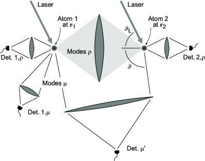
Figure 2: Detailed schematic of the physical system showing the detectors which correspond to the various measurements described in the text. Another detector $2,\mu$ would be placed in a location equivalent to that of detector $1,\mu$, to measure the emission of atom 2 individually.

IV.1 ”Multi-mode-resonator” regime

When $\gamma\tau\gg 1$, then the transient dynamics of the system is characterized by the two atoms exchanging a photonic excitation well localized in time. The excitation probabilities $P_{j}=|b_{e}^{(j)}(t)|^{2}$, with $b_{e}^{(j)}(t)$ given by Eqs. (16), are displayed in Fig. 3 as a function of time. One clearly sees that a photonic excitation propagates back and forth between the atoms, while its amplitude is damped due to the scattering into the external modes of the electromagnetic field. The shape of the photonic wave packet exchanged between the two atoms changes with time: with each bounce it acquires a more symmetric and broader shape, due to the frequency-dependent reflection by the atoms. The broadened wave packets increasingly overlap with time, such that interference between subsequent excitations may become visible for long times, as shown in the example of Fig. 4.

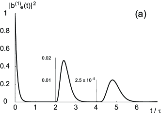
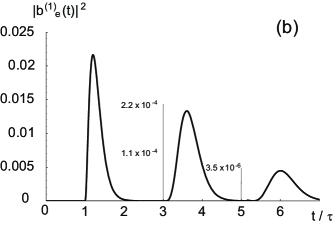
Figure 3: Excited state occupation of the atoms as a function of time in units of $\tau$, as given in Eq. (16), when initially atom 1 is excited. The other parameters are $\gamma\tau=10$, $\kappa=0.4$, and $\omega_{0}\tau=n\pi$. Note the change of vertical scale from each maximum to the next one.

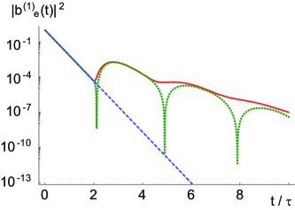
Figure 4: (Color online) Logarithmic plot of the excited state occupation of atom $1$ as a function of time in units of $\tau$, as given from Eq. (16). The curves correspond to the values $\omega_{0}\tau=n\pi$ (red solid line) and $\omega_{0}\tau=(2n+1/2)\pi$ (green dotted line) for $\kappa=0.4$ and $\gamma\tau=5$. The dashed line corresponds to $\kappa=0$ and is plotted for reference.

The effects of the coherent addition of the multiple scattering events become more visible by inspecting the time-dependent probability of emitting the photon into the external modes of the electromagnetic field. In the continuum limit of Eq. (III.3), it takes the form footnote:density

$$S(\omega,t)\propto|b_{g}(\omega,t)|^{2}~{}~{},$$ (33)

which for $t\to\infty$ coincides with the emission spectrum. An example of $S(\omega,t)$ is shown in Fig. 5. For times $t<\tau$, before scattering events can interfere, it exhibits a Lorentzian form like an atom in free space, while after a time $t>\tau$ it develops spectral modulation with peaks spaced by $1/2\tau$.

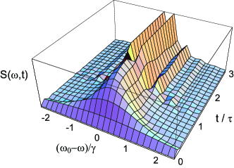
Figure 5: (Color online) Probability of emission of a photon, Eq. (33), as a function of frequency (in units of $\gamma$) and of time (in units of $\tau$), for the emission angle $\vartheta=\frac{\pi}{2}$ and the phase $\omega_{0}\tau=2n\pi$.

The effect of the distance between the atoms on their individual emission spectra is displayed in Figs. 6(a) and (b). In particular, the maxima of the spectra, spaced by the ”free spectral range” $1/2\tau$, shift according the optical distance between the atoms. The visibility of modulation is larger, the closer $\kappa$ is to unity.

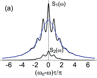
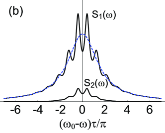
Figure 6: (Color online) Spectrum of the light emitted by atom $j$, $S_{j}(\omega)\propto\lim_{t\to\infty}|b^{(j)}_{g}(\omega,t)|^{2}$, as a function of the frequency (in units of $\pi/\tau$) for (a) $\omega_{0}\tau=n\pi$ and (b) $\omega_{0}\tau=(2n+1)\frac{\pi}{2}$. The parameters are $\kappa=0.4$ and $\gamma\tau=10$. The dashed blue line gives the spectrum of the atom when $\kappa=0$ and is plotted for comparison.

IV.2 ”Single-mode-resonator” regime

We now analyze the regime $\gamma\tau\ll 1$, in which several photon excitations are exchanged between the atoms during the natural lifetime of the excited state. In Fig. 7 the excited state populations of both atoms are displayed. As atom 1 is initially excited, atom 2 stays in the ground state until the instant $t=\tau$, after which its excited state occupation increases due to the interaction with the radiation from atom 1, see Fig.7(b). The excitation of atom 1 is damped like in free space until time $t=2\tau$, after which the damping rate is attenuated or enhanced depending on the relative interatomic distance, i.e. on $\omega_{0}\tau$. The effect of the relative phase between the multiple absorption-emission events is more evident when plotting the excitation probabilities on a logarithmic scale, as shown in Fig. 8.

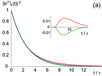
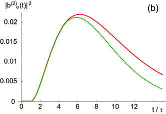
Figure 7: (Color online) Excited state occupation of (a) atom 1 and (b) atom 2 as a function of time (in units of $\tau$), as given in Eq. (16), when initially atom 1 is excited, and for $\omega_{0}\tau=n\pi$ (red solid line), $\omega_{0}\tau=(2n+1)\frac{\pi}{2}$ (green dotted line). The dashed blue line is the solution for $\kappa=0$) and is displayed for reference. The other parameters are $\gamma\tau=0.4$, $\kappa=0.4$. The red-solid and green-dotted lines in the inset of (a) display the difference between the value of $|b_{e}^{(1)}(t)|^{2}$ at $\omega_{0}\tau=n\pi$ and at $\omega_{0}\tau=(2n+1)\frac{\pi}{2}$, respectively, from the corresponding excited state occupation at $\kappa=0$ as a function of time.

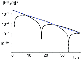
Figure 8: (Color online) Logarithmic plot of the excited state occupation of atom $1$ (solid line) and atom $2$ (dotted line) as a function of time (in units of $\tau$) for the initial state $|\Psi(0)\rangle=|e,g,0\rangle$. The other parameters are $\gamma\tau=0.4$ , $\kappa=0.4$ and $\omega_{0}\tau=(2n+1/2)\pi$. The blue dashed line shows the corresponding atomic excitation for $\kappa=0$ and is plotted for reference.

Figure 9(a) displays the emission probability $S(\omega,t)$ as a function of frequency and time, showing that it is always a single-peaked curve, whose width varies with time. Figure 9(b) displays the emission spectrum of the first atom in comparison with the one in free space for different values of the parameter $\omega_{0}\tau$, showing that depending on the relative distance one can observe subradiant or superradiant emission. The atomic interaction is hence a retarded dipole-dipole interaction, mediated by the photonic excitation over the interatomic distance.

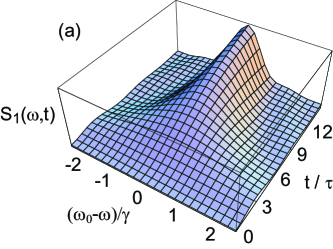
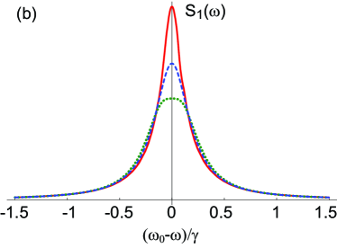
Figure 9: (Color online) (a) Probability of emission of a photon by atom 1, $S_{1}(\omega,t)\propto|b_{g}^{(1)}(\omega,t)|^{2}$, as a function of the frequency of the emitted photon (in units of $\gamma$) and of time (in units of $\tau$) for $\omega_{0}\tau=n\pi$. (b) Spectrum of emission for atom 1, $S_{1}(\omega)$, for $\omega_{0}\tau=n\pi$ (red solid line) and $\omega_{0}\tau=(2n+1)\frac{\pi}{2}$ (green solid line). The other parameters are $\gamma\tau=0.4$ and $\kappa=0.4$. The dashed blue line gives the emission spectrum in free space and is plotted for comparison.

IV.3 Two atoms vs. single atom

The cases studied so far share several analogies with the radiative properties of a single atom in front of a mirror, analyzed for instance in Alber ; Dorner . In particular, in Alber Alber studied the dynamics of one photon coupled to one atom at the center of a spherically symmetric cavity with perfect reflectivity. Depending on the radius of the cavity mirror, and thus on the time the photon needs to travel to the mirror and back in relation to the atomic decay time, Alber defines the small- and large-cavity limit, whereby in the first case the atom-cavity system is characterized by a delocalized excitation, while in the second case a photonic wave packet propagates back and forth exciting periodically the atom. Although our system is a low-quality resonator, the multi-mode cavity that the two atoms form for $\gamma\tau\gg 1$ is analogous to the large-cavity limit in Alber .

A very close analogy exists between our system and the system discussed in Dorner , where Dorner and Zoller investigated the case of an atom interacting with its own light back-reflected by a distant mirror Dorner . In particular, the dynamics of two atoms exchanging photons via the lens share strong analogies with the one of an atom interacting with its mirror image, if one restricts the Hilbert space to only one excitation, and if the atoms are initially prepared in a symmetric state with $\alpha_{1}=\alpha_{2}=1/\sqrt{2}$ in Eq. (11). For this initial state, the time evolution of the excitation of one of the atoms is the same as the one of the atom in front of the mirror. The probability amplitude for photon emission, however, shows some differences between the two cases. Figure 10 displays the emission spectrum as a function of the emission angle and of the frequency. Here, the oscillation of the intensity as a function of the angle of emission $\vartheta$ is indeed a exclusive property of the two-atom case, arising from the fact that the light emitted from the two scatterers interferes in the far field.

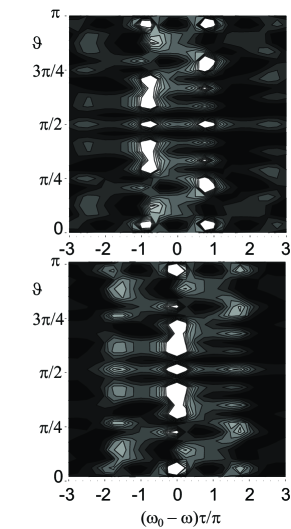
Figure 10: Contour plots of the emission spectrum from both atoms $S(\omega)$, Eq. (33), as a function of the frequency $\omega$ (in units of $\pi/\tau$) and of the angle of emission $\vartheta$, for the initial state $|\Psi(0)\rangle=\frac{1}{\sqrt{2}}(|e,g,0\rangle+|g,e,0\rangle)$. The other parameters are $\gamma\tau=10$, $\kappa=0.4$, and $\omega_{0}\tau=2n\pi$ (top panel), $\omega_{0}\tau=(2n+1)\pi$ (bottom panel).

V Light scattering

In this section we analyze the scattering properties of the system when the atoms are driven by a laser below saturation. In this case the time evolution of the excited state amplitudes, Eqs. (III.2), describes the photon exchange between the two atoms, which now additionally interferes with the incident laser light. For $\gamma\tau\gg 1$, step-wise dynamics with the characteristic time step $\tau$ are visible in the excited state occupation of each atom, as displayed in Fig. 11(a) and (b). For different distances between the atoms, and hence different phases of the various contributions, the discontinuities in the curves at multiples of $\tau$ show constructive or destructive interference, while for long times $t\gg\tau$ the excited-state population tends to a steady state value. In the limit $\gamma\tau\leq 1$, displayed in Fig. 11(c) and (d), the curves are smooth and tend to the same steady state values. This stationary value depends on the two phases $\varphi_{L}$ (the laser direction) and $\omega_{L}\tau$ (the optical path length between the atoms), according to

$$|c_{e}^{(1)}(t\to\infty)|^{2}=\frac{\Omega^{2}}{(\frac{\gamma^{2}}{4}+\Delta^{2})|1-K^{2}|^{2}}\left|1-K{\rm e}^{{\rm i}\varphi_{L}}\right|^{2}\,,$$ (34)

where $K$ is given in Eq. (32) and is proportional to the coupling strength $\kappa$ between the two ions. Eq. (34) does not depend on the parameter $\gamma\tau$, which affects only the transient dynamics. When the atoms are not coupled, $\kappa=0$, one recovers the free-space steady state value, as found for an atom which is driven by a weak laser Cohen-Tannoudji .

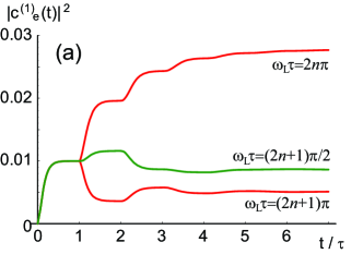
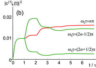
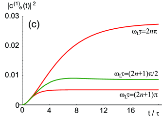
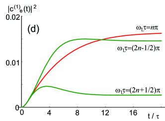
Figure 11: (Color online) Excited state population of atom $1$ when both atoms are driven by the laser, as evaluated from Eq. (III.2), as a function time (in units of $\tau$). The figures are evaluated for $\kappa=0.4$, $\Omega=0.05\gamma$, $\Delta=0$, and for $\gamma\tau=20$ (upper row) and for $\gamma\tau=1$ (lower row). The subplots (a) and (c) refer to the case $\varphi_{L}=(2n+1)\pi$, (b) and (d) to the case $\varphi_{L}=(2n-1/2)\pi$. The value of the phase $\omega_{L}\tau$ for each curve is explicitly given in the plots.

We note that for the specific value $\varphi_{L}=(2n+1)\pi$ we obtain

$$|c_{e}^{(1)}(\infty)|^{2}=\frac{\Omega^{2}}{\tilde{\gamma}_{L}^{2}/4+\tilde{\Delta}^{2}}\,,$$ (35)

which is the free-space formula with modified decay rate and detuning,

$$\tilde{\gamma} = \gamma\,(1-\kappa\cos\omega_{L}\tau)\,,$$

$$\tilde{\Delta} = \Delta-\kappa\frac{\gamma}{2}\sin\omega_{L}\tau\,.$$

This result coincides with the excited state population of a single atom subject to interference between the laser excitation and the light back-scattered from a mirror Dorner . This equivalence holds only for the particular value $\varphi_{L}=(2n+1)\pi$ but not in the general case.

In order to get some more insight, we analyze Eq. (34) for $\kappa\ll 1$. At first order in $\kappa$ the excited state population of the first atom takes the value

$$|c_{e}^{(1)}(t\to\infty)|^{2} \approx \frac{\Omega^{2}}{\gamma^{2}/4+\Delta^{2}}$$

$$\times \left(1+2\kappa A\cos\left[\omega_{L}\tau+\varphi_{L}-\phi\right]\right)\,,$$

with

$$A=\sqrt{\frac{\gamma^{2}/4}{\gamma^{2}/4+\Delta^{2}}}\,,$$

$$\tan\phi=\frac{2\Delta}{\gamma}\,.$$ (37)

The result for atom 2 is found from Eq. (V) by swapping the subscripts $1\leftrightarrow 2$, i.e. by changing the sign of $\varphi_{L}$. Equation (V) shows how the excited state population is enhanced or suppressed as the parameter $\omega_{L}\tau$ is changed. This change in the atomic spontaneous emission rate, as well as a shift of the atomic resonance frequency, both controlled by the parameter $\omega_{L}\tau$, are manifestations of the modification of the radiative properties of the atoms due to their mutual interaction. Analogous frequency shifts in a single atom interacting with itself via a mirror have been experimentally observed by Wilson et al. Wilson .

V.1 Intensity of the scattered light

Let us now consider the intensity of the light scattered by the laser-driven atoms, for several of the measurement set-ups illustrated in Fig. 2.

First we consider the situation that the detection apparatus resolves the atomic positions and therefore sums up incoherently the photons emitted by the atoms (detector $1,\mu$ plus detector $2,\mu$). Then the detection rate is $\Gamma_{\mu}=\Gamma_{1,\mu}+\Gamma_{2,\mu}$, whereby $\Gamma_{j,\mu}=\lim_{t\to\infty}|c_{g}^{(j,\mu)}(t)|^{2}/t$. Using Eq. (27) we find

$$\Gamma_{1,\mu}=\Gamma_{2,\mu}=2\pi\delta(\omega_{\mu}-\omega_{L})\frac{g_{\mu}^{2}\Omega^{2}}{(\frac{\gamma^{2}}{4}+\delta_{\mu}^{2})}\frac{\left|1-K{\rm e}^{{\rm i}\varphi_{L}}\right|^{2}}{|1-K^{2}|^{2}}\,,$$ (38)

where $K$ is given in Eq. (32). For $K=0$, i.e. in absence of the optical element coupling the two atoms, the signal reproduces the free-space resonance curve of the atomic dipole. For $K\neq 0$ it shows two modulations, with the phase $2\omega_{L}\tau$ (through $K^{2}$ in the denominator) and with the phase $\omega_{L}\tau+\varphi_{L}$ (in the numerator). The first one corresponds to previously emitted light returning to the same atom after scattering from the other one, the other modulation is produced by scattered laser light arriving from the other atom. In general, the modulations show how the scattering of a single atom is modified by the presence of another identical scatterer at a fixed distance. The maximum enhancement, when all scattering terms add up coherently, is found for $2\omega_{L}\tau=2\pi$, $\varphi_{L}=0$ and $\Delta=0$, and is equal to $(1+\kappa)/(1-\kappa)$. For $\kappa=0.2$ it gives an enhancement of the signal of the order to 150%, as displayed in Fig. 12. For the case of a single atom interacting with itself via a distant mirror, analogous signals have been experimentally observed in Refs. Eschner2001 ; Wilson .

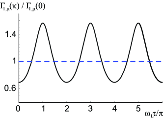
Figure 12: (Color online) Intensity of the light emitted by one atom into free space, as a function of $2\omega_{L}\tau$ and for $\kappa=0.2$, when the system is driven by a laser at frequency $\omega_{L}=\omega_{0}$ and at $\varphi_{L}=0$. The intensity is normalized to the value obtained without coupling, $\kappa=0$ (blue dashed line).

When the light emitted by the two atoms is superposed coherently on a detector (labeled $\mu^{\prime}$ in Fig. 2), the system is analogous to a double-slit set-up Itano with the important difference that the atoms additionally interact by photon exchange via the lens. In this case, the corresponding detection rate is $\Gamma_{\mu}^{\prime}=\lim_{t\to\infty}|c_{g}^{(\mu)}(t)|^{2}/t$ and takes the explicit form

$$\Gamma_{\mu}^{\prime}=8\pi\delta(\omega_{\mu}-\omega_{L})\frac{g_{\mu}^{2}\Omega^{2}}{(\frac{\gamma^{2}}{4}+\delta_{\mu}^{2})|1-K^{2}|^{2}}\left|\cos[({\bf k_{L}}-{\bf k}_{\mu})\cdot({\bf r_{1}}-{\bf r_{2}})/2]-K\cos[({\bf k_{L}}+{\bf k}_{\mu})\cdot({\bf r_{1}}-{\bf r_{2}})/2]\right|^{2}\,.$$ (39)

For $K=0$, the observed spatial interference is the one of a double-slit set-up with two coherently driven sources Itano ; Skornia . When $K\neq 0$, these properties are modified by the multiple scattering. An important special case is when the direction of emission is ${\bf k_{\mu}}=-{\bf k_{L}}$, corresponding to the coherent backscattering direction Wickles , where one always finds a spatial maximum of the scattered intensity.

We now consider a set-up in which one observes the modes $\rho$, through which the atoms interact (detectors $1,\rho$ and $2,\rho$ in Fig. 2). This corresponds to the measurement arrangement in Eschner2001 . In this case, the rate at detector $1,\rho$ is given by $\Gamma_{1,\rho}=\lim_{t\to\infty}|c_{g}^{(1,\rho)}(t)+c_{g}^{(2,\rho^{\prime})}(t)|^{2}/t$, superposing the light emitted by atom 1 directly into the detector with the light emitted by atom 2 towards atom 1, and then into the detector, whereby ${\bf k}_{\rho}$ and ${\bf k}_{\rho}^{\prime}$ are transformed into each other by the lens. It reads

$$\Gamma_{1,\rho}=8\pi\delta(\omega_{\rho}-\omega_{L})\frac{g_{\rho}^{2}\Omega^{2}}{(\frac{\gamma^{2}}{4}+\delta_{\rho}^{2})|1-K^{2}|^{2}}\left|\cos[(\varphi_{L}-\omega_{L}\tau)/2]-K\cos[(\varphi_{L}+\omega_{L}\tau)/2]\right|^{2}\,,$$ (40)

where we used that ${\bf k}_{\rho^{\prime}}\cdot{\bf r_{2}}-{\bf k}_{\rho}\cdot{\bf r_{1}}\to\omega_{L}\tau$ via the optical element. The corresponding rate $\Gamma_{2,\rho}$ is found by changing the sign of $\varphi_{L}$ in Eq. (40). The total rate $\Gamma_{\rho}^{(0))}=\Gamma_{1,\rho}^{(0)}+\Gamma_{2,\rho}^{(0)}$ was measured in Ref. Eschner2001 in an optical set-up, which was characterized by small values of $\kappa$. Taking $\kappa\ll 1$, the total rate $\Gamma_{\rho}^{(0)}$ reads

$$\Gamma_{\rho}^{(0)}\propto 1+\cos\varphi_{L}\cos\omega_{L}\tau-\kappa A\left[\cos\phi+2\cos\varphi_{L}\cos(\omega_{L}\tau-\phi)+\cos(2\omega_{L}\tau-\phi)\right]+{\rm O}(\kappa^{2})\,,$$ (41)

where we omitted global constant factors, and $\phi$ and $A$ are defined in Eq. (V). We observe that at zero order in $\kappa$ an interference pattern appears as a function of $\omega_{L}\tau$, i.e. by changing the optical path between the ions. This is the classical interference of the light elastically scattered from both atoms into the same detector. The interference has visibility

$${\mathcal{V}}_{1}=|\cos\varphi_{L}|\,,$$ (42)

which is maximum when $\varphi_{L}=n\pi$, with $n$ integer, and which vanishes when $\varphi_{L}=(2n+1)\pi/2$. This is a consequence of summing the signals from the two detectors, whose individual interference patterns may be shifted depending on $\varphi_{L}$. It provides an explanation for the low contrast interference observed in the experiment of Ref. Eschner2001 .

The vanishing contrast when the two signals are perfectly anti-correlated provides a condition where the higher order effects in $\kappa$, and thereby the interaction of the atoms, are particularly evident. Choosing this specific condition, by varying the optical path length between the ions one observes an interference pattern at twice the frequency of the classical interference, i.e. oscillating with $2\omega_{L}\tau$, with a shift $\phi$ determined by the detuning $\Delta$, and whose visibility is given by

$${\mathcal{V}}_{2}=\kappa A=\frac{\kappa}{\sqrt{1+4\Delta^{2}/\gamma^{2}}}\,,$$ (43)

where we used Eq. (V). The visibility is maximum at atomic resonance. The doubled frequency of the interference (compared to the classical one) with the interatomic distance shows that it is caused by two partial waves originating from the same atom, one reaching directly the detector and the other being back-scattered once by the other atom. Analogously, processes where the same wave is scattered $n$ times by the atoms give rise to interference terms with frequency $n\omega_{L}\tau$ and at higher order in $\kappa$.

V.2 Intensity-Intensity Correlations

We now study the intensity-intensity correlations in this set-up, assuming that two detectors are placed in the far field of the scattered light at positions ${\bf x_{1}}$ and ${\bf x_{2}}$ (corresponding to two detectors $\mu^{\prime}$ in Fig. 2 at angles $\vartheta_{1}$ and $\vartheta_{2}$). We denote by ${\mathcal{G}}^{(2)}({\bf x_{1}},t;{\bf x_{2}},t+t^{\prime})$ the (un-normalized) intensity-intensity correlation function for measuring a photon at time $t$ and position ${\bf x_{1}}$, and another at ${\bf x_{2}}$ after an interval $t^{\prime}$. It reads Skornia

$${\mathcal{G}}^{(2)}({\bf x_{1}},t;{\bf x_{2}},t+t^{\prime})=\sum_{\zeta,\nu,\lambda,\rho=1,2}{\rm e}^{{\rm i}k\left(({\bf r}_{\lambda}-{\bf r}_{\nu})\cdot{\bf\hat{x}_{1}}+({\bf r}_{\xi}-{\bf r}_{\zeta})\cdot{\bf\hat{x}_{2}}\right)}~{}\langle\hskip 2.84544pt\sigma^{+}_{\lambda}(t)\sigma^{+}_{\xi}(t+t^{\prime})\sigma_{\nu}(t+t^{\prime})\sigma_{\zeta}(t)\hskip 2.84544pt\rangle\,,$$ (44)

where $k=|{\bf k_{L}}|$ and ${\bf\hat{x}}={\bf x}/|{\bf x}|$. Assuming that the atoms are driven by the laser and have reached the steady state, Eq. (44) depends solely on the time $t^{\prime}$ elapsed between the two detection events. In this limit, we evaluate its explicit form in perturbation theory for the atom-photon interaction, and find the expression

$$G^{(2)}(\varphi_{1},\varphi_{2};t^{\prime}) = \left.\frac{16\Omega^{4}}{(\gamma^{2}+4\Delta^{2})^{2}}\frac{1}{|1-K^{2}|^{2}}\right|\left(1+{\rm e}^{{\rm i}(\varphi_{1}+\varphi_{L})}-K({\rm e}^{{\rm i}\varphi_{1}}+{\rm e}^{{\rm i}\varphi_{2}})\right)$$

$$\times \left[\left(1+{\rm e}^{{\rm i}(\varphi_{2}+\varphi_{L})}\right)\sum_{k}H_{2k}(t^{\prime},\omega_{L})+({\rm e}^{{\rm i}\varphi_{L}}+{\rm e}^{{\rm i}\varphi_{2}})\sum_{k}H_{2k+1}(t^{\prime},\omega_{L})\right]$$

$$+ \left.{\rm e}^{{\rm i}(\varphi_{L}-\Delta t^{\prime})}(1-K\cos\varphi_{L})\left[({\rm e}^{{\rm i}\varphi_{1}}+{\rm e}^{{\rm i}\varphi_{2}})\sum_{k}I_{2k}+\left(1+{\rm e}^{{\rm i}(\varphi_{1}+\varphi_{2})}\right)\sum_{k}I_{2k+1}\right]\right|^{2}\,,$$

where we have set

$$\varphi_{j}=k({\bf r_{2}}-{\bf r_{1}})\cdot{\bf\hat{x}_{j}}=kd\cos\vartheta_{j}$$ (46)

and defined $G^{(2)}(\varphi_{1},\varphi_{2};t^{\prime})=\mathcal{G}^{(2)}({\bf x_{1}},t;{\bf x_{2}},t+t^{\prime})$. The detailed derivation of Eq. (V.2) is reported in Appendix C. For $\kappa=0$, i.e. in absence of coupling, $G^{(2)}$ exhibits an interference pattern as a function of the distance $|{\bf x_{2}}-{\bf x_{1}}|$ between the detectors. Such interference emerges from two indistinguishable paths of two-photon emission. It has first been predicted in Mandel for the case of two independent quantum sources, and generalized in Skornia for the light scattered by two trapped atoms illuminated by a laser. In particular, the result of Skornia for weak laser intensity is obtained from Eq. (V.2) by taking the limit $\kappa\to 0$ and setting $\Delta=0$ Footnote .

We now consider this spatial interference pattern at $t^{\prime}=0$, for $\varphi_{L}=0$ and $\Delta=0$, but keeping $\kappa\neq 0$. For these parameters it takes the form

$$G^{(2)}(\varphi_{1},\varphi_{2};0)=\frac{64\Omega^{4}}{\gamma^{4}}~{}\frac{\cos^{2}(\varphi_{1}-\varphi_{2})/2}{1+\kappa^{2}+2\kappa\cos\omega_{0}\tau}.$$ (47)

In particular, Eq. (47) vanishes for $|\varphi_{1}-\varphi_{2}|=(2n+1)\pi$, showing strong antibunching at these points. Similarly, bunching is encountered whenever the condition $|\varphi_{1}-\varphi_{2}|=2n\pi$ is fulfilled. We note, moreover, that since this signal depends only on the difference $\varphi_{1}-\varphi_{2}$, there exists a finite probability of measuring two photons simultaneously at the positions of the screen which are the dark fringes of the first-order interference pattern, $\varphi_{j}=(2n+1)\pi$. This behaviour has been discussed in Skornia-2 : it is connected to the fact that saturation effects diminish the contrast of the first-order correlation function, leading to a non-vanishing probability of measuring a photon at these detector positions. The probability to measure the first photon in the dark fringe is essentially proportional to the occupation of the collective state $|e_{1},e_{2}\rangle$, and the first detection projects the atoms into the antisymmetric Dicke state $|\psi(0)\rangle=\frac{1}{\sqrt{2}}(|e,g\rangle-|g,e\rangle)$, which is an entangled state of the two distant atoms.

The denominator of Eq. (47) shows how the spatial interference pattern is modified due to the atom-atom interaction by multiple photon scattering, and how this modification depends on the phase $\omega_{L}\tau$.

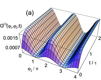
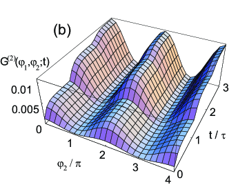
Figure 13: (Color online) $G^{(2)}(\varphi_{1},\varphi_{2};t)$ as a function of time $t$ (in units of $\tau$) and $\varphi_{2}$ for $\varphi_{1}=2n\pi$. The subplots refer to the cases (a) $\kappa=0$ (no interaction) and (b) $\kappa=0.4$. The other parameters are $\Omega=0.05\gamma$, $\Delta=0$, $\varphi_{L}=0$, $\gamma\tau=20$, and $\omega_{0}\tau=(2n+1)\pi$.

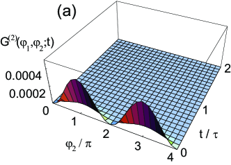
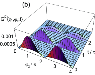
Figure 14: (Color online) Same as Fig. 13 but with $\varphi_{1}=(2n+1)\pi$. The curves in (b) at $t>\tau$ are magnified by a factor 30.

Figures 13 and 14 display the intensity-intensity correlation function versus $t^{\prime}$ and $\varphi_{2}$, for the situation $\gamma\tau\gg 1$. The two figures correspond to the bright ($\varphi_{1}=2n\pi$) and dark ($\varphi_{1}=(2n+1)\pi$) fringes of the first-order correlation function, and both show the cases $\kappa=0$ and $\kappa=0.4$, for comparison. One clearly observes the effect due to multiply scattered photons, giving rise to abrupt changes in the slope of the correlation function at multiples of $\tau$. Hence, the interference due to multiple scattering enhances or suppresses the probability of measuring the second photon at a certain time interval. Related effects have been observed in a single-atom interference experiment in Ref. Dubin07 . We now analyze this latter property setting $\varphi_{1}=(2n+1)\pi$, i.e. when the first detector is set at a dark fringe of the first-order correlation function: in Fig. 14(a) one sees that for $\kappa=0$ the second order correlation function is different from zero at $t^{\prime}=0$ and for $\varphi_{2}\neq 2n\pi$, and it vanishes after a transient time of the order $1/2\gamma$, corresponding to the lifetime of the collective state $|e,e\rangle$ Skornia-2 . For $\kappa=0.4$, Fig. 14(b), one observes ”revivals” when the time between the two detections is a multiple of $\tau$, and whose amplitude is strongly damped as a function of time. Inspecting Eq. (V.2) for these specific parameters, we find that at short times the correlation function behaves as

$$G^{(2)}(\varphi_{1},\varphi_{2};t^{\prime})\Bigl{|}_{\varphi_{1}=(2n+1)\pi,t^{\prime}\ll\tau}\approx$$ (48)

$$\frac{32\Omega^{4}(1-\cos\varphi_{2})}{\gamma^{4}(1+\kappa^{2}+2\kappa\cos\omega_{0}\tau)}\left|\sum_{k}(-1)^{k}I_{k}\right|^{2}\,,$$

and it is essentially proportional to the probability of measuring the atoms in the state $|\psi(t^{\prime})\rangle$, obtained by freely evolving the initial state $|\psi(0)\rangle=\frac{1}{\sqrt{2}}(|e,g\rangle-|g,e\rangle)$, according to Eq. (16).

For longer times, $t^{\prime}>\tau$, the second-order correlation function scales with $\kappa^{2}$ and takes the form

$$G^{(2)}(\varphi_{1},\varphi_{2};t^{\prime})\Bigl{|}_{\varphi_{1}=(2n+1)\pi,t^{\prime}>\tau}$$ (49)

$$\approx\frac{64\Omega^{4}(1-\cos^{2}\varphi_{2})}{\gamma^{4}(1+\kappa^{2}+2\kappa\cos\omega_{0}\tau)}\Bigl{|}K\sum_{k}H_{k}(\omega_{L},t^{\prime})\Bigr{|}^{2}\,,$$

which is essentially proportional to the stationary excited-state occupation of the atoms given in Eq. (III.2).

While the limit $\gamma\tau\gg 1$ is characterized by ”revivals” of the correlation function versus the time $t^{\prime}$ between two photon detections, in the limit $\gamma\tau\leq 1$ one observes a smooth decay of the correlation function with $t^{\prime}$, whereby its decay rate is modified depending on whether the multiply scattered waves interfere constructively or destructively at the atom. A comparison between the two regimes is shown in Fig. 15.

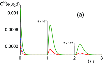
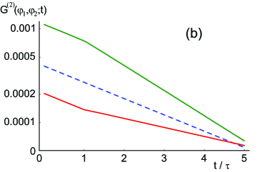
Figure 15: (Color online) $G^{(2)}(\varphi_{1},\varphi_{2};t)$ as a function of time for $\varphi_{1}=\varphi_{2}=(2n+1)\pi$ and $\kappa=0.4$ when (a) $\gamma\tau=20$ (note the change of vertical scale from each maximum to the next one) and (b) $\gamma\tau=0.4$. The red-solid (bottom) and green-solid (top) curves are evaluated at $\omega_{0}\tau=2n\pi$ and $(2n+1)\pi$, respectively. The blue dashed line represents the behaviour at $\kappa=0$ and is plotted for reference. The other parameters are $\Omega=0.05\gamma$, $\Delta=0$, $\varphi_{L}=0$.

To conclude this section, one of the main features associated with photon-mediated atom-atom interaction is that the intensity-intensity correlation exhibits an enhanced or suppressed probability to measure a second photon as a function of the time after the first detection. This behaviour is due to interference between the various paths of multiple scattering, and can be interpreted as a combined photonic-atomic excitation which is stored inside the system. In view of the interpretation by Skornia-3 ; Metz , one can say that for a transient time the system develops and stores entanglement and correlations, determined by the strength of the interaction $\kappa$, until the atoms finally dissipate the excitation into free space. In the future, it would be interesting to consider these dynamics in a quantum jump picture Skornia-3 . This could open the possibility of implementing schemes for entangling atoms in this kind of set-up, as proposed in Metz .

VI Conclusions

We have studied the photonic properties of two atoms which are coupled by radiation via an optical element such as, e.g., a lens or an optical fiber focussing a relevant fraction $\kappa$ of electromagnetic field modes from one atom to the other. Signatures of multiple scattering of photons between the atoms are observed in the first-order and second-order coherence of the scattered light. These features show that the presence of the second atom substantially modifies the radiative properties of the first one, even when the atoms are separated by a distance $d$ much larger than the light wavelength $\lambda$.

The efficiency of the interaction, which for two atoms in free space scales with $\lambda/d$, is determined by $\kappa$ when an optical system mediates the coupling. The atom-atom distance $d$ plays a new role, separating two regimes where the delay of the interaction $\tau=d/c$ is smaller or larger than the atomic decay time $1/\gamma$. In these two regimes $\gamma\tau<1$ and $\gamma\tau>1$, the coupled two-atom system shows characteristics of a single- or multi-mode resonator, respectively, with mirrors of low reflectivity $\kappa$ and bandwidth $\gamma$.

In this article we considered the limit in which the atoms are weakly driven by the laser, and we neglected the effect of atomic motion. It should be remarked that localization of the atoms within a wavelength of the scattered light is a relevant requirement for observing the interference effects arising from multiple scattering. In fact, atomic motion gives rise to a dephasing in the signal, which can be interpreted as which-way information imprinted by the photon recoil on the scattering atom Wickles ; Eschner2003 ; Englert . Nevertheless, when the recoil of the atom in each photon scattering event is taken into account, correlations between the atomic motion and the light are established Eberly . In particular, mechanical effects between the distant atoms arise, which are mediated and retarded by the optical coupling Bushev2004 ; iacopini93 . It is interesting to consider whether such effects may lead to novel collective behaviour of atomic center-of-mass and photonic variables, in analogy to collective dynamics predicted for cold atoms inside resonators Ritsch .

Appendix A

We formally integrate Eqs. (9b) and (9c) using the initial condition $b_{g}^{(\ell)}(0)=0$. Inserting the result into Eq. (9a) yields

$$\dot{b}_{e}^{(1)}(t)=-\sum_{\ell=\mu,\rho}g_{\ell}^{2}\int_{0}^{t}{\rm d}t^{\prime}e^{{\rm i}(\omega_{0}-\omega_{\ell})(t-t^{\prime})}b_{e}^{(1)}(t^{\prime})$$ (50)

$$-\sum_{\rho}g_{\rho}^{2}\int_{0}^{t}{\rm d}t^{\prime}e^{{\rm i}(\omega_{0}-\omega_{\rho})(t-t^{\prime})}{\rm e}^{{\rm i}{\bf k_{\rho}}\cdot({\bf r_{1}}-{\bf r_{2}})}b_{e}^{(2)}(t^{\prime})\,,$$

where the equation for $b_{e}^{(2)}(t)$ is found by swapping the indexes $1$ and $2$ in Eq. (50). We see that the differential equation for the probability amplitude $b_{e}^{(1)}(t)$ depends linearly on the probability amplitude $b_{e}^{(2)}(t^{\prime})$ for the excited state of atom $2$. Such dependence is due to the common modes $\rho$ which mediate the interaction between the two atoms. In absence of the second atom, the equation reduces to the well known equations describing the radiative decay of a two-level atom in free space Cohen-Tannoudji .

The first term on the right-hand side (RHS) of Eq. (50) can be rewritten in a compact way by converting the sum over the modes into an integral. Using the Wigner-Weisskopf approximation one obtains Milonni

$$\dot{b}_{e}^{(1)}(t)=-\frac{\gamma}{2}b_{e}^{(1)}(t)$$ (51)

$$-\int_{0}^{t}{\rm d}t^{\prime}b_{e}^{(2)}(t^{\prime})\sum_{\rho}g_{\rho}^{2}{\rm e}^{{\rm i}{\bf k_{\rho}}\cdot({\bf r_{1}}-{\bf r_{2}})}{\rm e}^{{\rm i}(\omega_{0}-\omega_{\rho})(t-t^{\prime})}\,,$$

where $\gamma=D^{2}\omega_{0}^{3}/(3\pi\varepsilon_{0}\hbar c^{3})$ is the free-space decay rate Cohen-Tannoudji . The second term on the RHS of Eq. (51) corresponds to the sum of the modes mapped from one atom into the other by the optical setup. Let us consider a lens between the atoms collecting a solid angle $\delta\Omega_{0}$ of modes with aperture $\theta_{0}$. Converting the sum over the modes into an integral, the sum over the modes $\rho$ in Eq. (51) can be rewritten as

$$\sum_{\rho}g_{\rho}^{2}{\rm e}^{{\rm i}{\bf k_{\rho}}\cdot({\bf r_{1}}-{\bf r_{2}})}{\rm e}^{{\rm i}(\omega_{0}-\omega_{\rho})(t-t^{\prime})}\to$$

$$\frac{1}{2(2\pi)^{3}\varepsilon_{0}\hbar c^{3}}\int_{0}^{\infty}{\rm d}\omega\omega^{3}{\rm e}^{{\rm i}(\omega_{0}-\omega)(t-t^{\prime})}$$

$$\times\int_{\delta\Omega_{0}}{\rm d}\Omega{\rm e}^{{\rm i}{\bf k}\cdot({\bf r_{1}}-{\bf r_{2}})}\left(D^{2}-\frac{|{\bf D}\cdot{\bf k}|^{2}}{k^{2}}\right)\,.$$ (52)

Since optics compensate for the phase difference between the various modes, we take

$${\rm e}^{{\rm i}{\bf k}\cdot({\bf r_{1}}-{\bf r_{2}})}\rightarrow e^{{\rm i}\omega\tau}\,,$$ (53)

where $\tau$ is defined in Eq. (1), and is the time a photon emitted inside the solid angle $\delta\Omega_{0}$ needs to cover the distance between one atom and the other via optical setup. Using Eq. (52) into Eq. (51), we can now make the Wigner-Weisskopf approximation and obtain Eq. (10).

Appendix B

We consider the terms of Eq. (27). Let us introduce the simple relation

$$\mathcal{I}=\int_{0}^{t}{\rm d}t^{\prime}{\rm e}^{{\rm i}(\omega_{L}-\omega_{\mu})t^{\prime}}H_{k}(t^{\prime},\omega_{\mu})$$

$$=\frac{(-\kappa\frac{\gamma}{2})^{k}}{k!}{\rm e}^{{\rm i}\omega_{L}k\tau}\Theta(t-k\tau)\int_{0}^{t-k\tau}{\rm d}x{\rm e}^{{\rm i}(\omega_{L}-\omega_{\mu})x}x^{k}G_{k}(\alpha x)\,,$$

with $\alpha=\frac{\gamma}{2}+{\rm i}\delta_{\mu}$ and where we used Eq. (20). Using the definition of the confluent hypergeometric function Abramowitz ,

$${}_{1}F_{1}(a,b,z)=1+\frac{a}{b}z+\frac{a(a+1)}{b(b+1)}\frac{z^{2}}{2!}+\ldots\,,$$ (55)

we rewrite Eq. (21) as

$$G_{k}(s)=\left\{\begin{array}[]{ll}1-e^{-s}&\mbox{if $k=0$};\\ -\sum_{n=0}^{\infty}\frac{n}{n+k}\frac{(-s)^{n}}{n!}&\mbox{if $k\neq 0$}.\end{array}\right.$$ (56)

or equivalently

$$G_{k}(s) = \frac{k!}{s^{k}}-(-1)^{k}s\frac{\partial^{k}}{\partial s^{k}}\frac{e^{-s}}{s}\,,$$ (57)

whereby

$$(-1)^{k}s\frac{\partial^{k}}{\partial s^{k}}\frac{e^{-s}}{s}={\rm e}^{-s}\sum_{n=0}^{k}\frac{k!}{(k-n)!}s^{-n}.$$ (58)

We use Eq. (57) in Eq. (B), and obtain

$$\mathcal{I}=\frac{(-\kappa\frac{\gamma}{2}{\rm e}^{{\rm i}\omega_{L}\tau})^{k}}{\alpha^{k}}\Theta(t-k\tau)\left(\int_{0}^{t-k\tau}{\rm d}x{\rm e}^{{\rm i}(\omega_{L}-\omega_{\mu})x}-S_{k}\right)\,,$$ (59)

with

$$S_{k}(t)=\frac{(-1)^{k}}{k!}\int_{0}^{t-k\tau}{\rm d}x{\rm e}^{-{\rm i}\Delta_{\mu}x}x^{k+1}\frac{\partial^{k}}{\partial{x}^{k}}\frac{e^{-\alpha x}}{x}\,.$$ (60)

As we are interested in evaluating the scattering processes for long times, $t\to\infty$, we neglect the term $k\tau$ in the upper bound of the integral and take the Heaviside function to be one. The first term inside the parentheses on the RHS of Eq.(59) gives

$$\int_{0}^{t}{\rm d}x\,{\rm e}^{-{\rm i}\Delta_{\mu}x} = {\rm e}^{-{\rm i}\Delta_{\mu}t/2}2\pi\delta^{(t)}(\Delta_{\mu})\,.$$ (61)

In order to evaluate the term (60) we use the relations Eq. (58) and

$$\int_{0}^{t}{\rm d}x\,x^{j}{\rm e}^{-\alpha x} = \frac{j!}{\alpha^{j+1}}-\frac{j!{\rm e}^{-\alpha t}}{\alpha^{j+1}}\sum_{l=0}^{j}\frac{(\alpha t)^{l}}{l!}\,,$$

in Eq. (60), which then reads

$$S_{k}(t) = \sum_{j=0}^{k}\frac{\alpha^{j}}{(\alpha+{\rm i}\Delta_{\mu})^{j+1}}$$

$$\times\left(1-{\rm e}^{-(\alpha+{\rm i}\Delta_{\mu})t}\sum_{l=0}^{j}\frac{(\alpha+{\rm i}\Delta_{\mu})^{l}t^{l}}{l!}\right)\,.$$

In particular,

$$\sum_{k=0}^{\infty}\begin{array}[]{l}K^{\prime 2k}S_{2k}\\ K^{\prime 2k+1}S_{2k+1}\end{array}=\frac{1}{2}\left[\sum_{k=0}^{\infty}K^{\prime k}S_{k}\pm(-1)^{k}K^{\prime k}S_{k}\right]\,,$$ (62)

where

$$\sum_{k=0}^{\infty}(\pm 1)^{k}K^{\prime k}S_{k}\approx\frac{1}{(1\mp K^{\prime})(\alpha+{\rm i}\Delta_{\mu}\mp\alpha K^{\prime})}\,,$$ (63)

with $K^{\prime}=-\kappa\frac{\gamma}{2}{\rm e}^{{\rm i}\omega_{L}\tau}/(\frac{\gamma}{2}+{\rm i}\delta_{\mu})$, and where we used the Cauchy-Product for absolute convergent series, thereby neglecting the vanishing exponentials as we consider the long time limit.
In the long-time limit, using that $\lim_{t\to+\infty}\delta^{(t)}(x)=\delta(x)$ we finally arrive to the relation in Eq. (31).

Appendix C

Starting from Eq. (44) we calculate the second order correlation function of two atoms, which are weakly driven by the laser and both scatter towards the detector. In the reference frame rotating at the laser frequency, assuming that the initial state is the atomic ground state, we rewrite Eq. (44) as

$${\mathcal{G}}^{(2)}({\bf x_{1}},t;{\bf x_{2}},t+t^{\prime})=$$ (64)

$$\|(\sigma_{1}+\sigma_{2}e^{{\rm i}\varphi_{2}})U(t^{\prime})(\sigma_{1}+\sigma_{2}e^{{\rm i}\varphi_{1}})U(t)|g,g,0\rangle\|^{2}\,,$$

where the correlation function is evaluated at lowest order in perturbation theory in the atom-photon interactions. The operator $U(t)$ is the total evolution operator,

$$U(t)=\exp(-{\rm i}H^{\prime}t/\hbar)\,,$$

with $H^{\prime}$ given in Eq. (5), which is to be expanded in power series of the interactions $V_{\rm emf}$ and $V_{L}$. At lowest, non-vanishing order, Eq. (64) can be rewritten as

$${\mathcal{G}}^{(2)}({\bf x_{1}},t;{\bf x_{2}},t+t^{\prime})$$

$$=\left|\left(A_{1}(t)+A_{2}(t)e^{{\rm i}\varphi_{1}}\right)\left(A_{1}(t^{\prime})+A_{2}(t^{\prime})e^{{\rm i}\varphi_{2}}\right)+B(t)\right.$$

$$\times\left.\left[C_{11}(t^{\prime})+{\rm e}^{{\rm i}\varphi_{1}}C_{21}(t^{\prime})+{\rm e}^{{\rm i}\varphi_{2}}\left(C_{12}(t^{\prime})+C_{22}(t^{\prime}){\rm e}^{{\rm i}\varphi_{1}}\right)\right]\right|^{2}\,,$$

where the coefficients $A_{j}$ and $B$ are the transition amplitudes

$$A_{1}(t)=\langle e,g,0|U(t)|g,g,0\rangle=c_{e}^{(1)}(t)\,,$$ (66)

$$A_{2}(t)=\langle g,e,0|U(t)|g,g,0\rangle=c_{e}^{(2)}(t)\,,$$ (67)

$$B(t)=\langle e,e,0|U(t)|g,g,0\rangle\,,$$ (68)

where $c_{e}^{(j)}(t)$ is given in Eq. (III.2), while the probability amplitudes $C_{ji}$ are defined as

$$C_{11} = \langle e,g,0|U(t)|e,g,0\rangle$$

$$= e^{-{\rm i}\Delta t}b_{e}^{(1)}(t)\hskip 14.22636pt\mbox{with}\hskip 14.22636ptb_{e}^{(1)}(0)=1\,,$$

$$C_{12} = \langle g,e,0|U(t)|e,g,0\rangle$$

$$= e^{-{\rm i}\Delta t}b_{e}^{(2)}(t)\hskip 14.22636pt\mbox{with}\hskip 14.22636ptb_{e}^{(1)}(0)=1\,,$$

$$C_{21} = \langle e,g,0|U(t)|g,e,0\rangle$$

$$= e^{-{\rm i}\Delta t}b_{e}^{(1)}(t)\hskip 14.22636pt\mbox{with}\hskip 14.22636ptb_{e}^{(2)}(0)=1\,,$$

$$C_{22} = \langle g,e,0|U(t)|g,e,0\rangle$$

$$= e^{-{\rm i}\Delta t}b_{e}^{(2)}(t)\hskip 14.22636pt\mbox{with}\hskip 14.22636ptb_{e}^{(2)}(0)=1\,,$$

with $b_{e}^{(j)}(t)$ given in Eq. (16). We evaluate the coefficient $B(t)$ in second-order perturbation theory, hence obtaining

$$B(t) = -{\rm i}\Omega\int_{0}^{t}dt^{\prime}{\rm e}^{-(2{\rm i}\Delta+\gamma)(t-t^{\prime})}$$ (69)

$$\times\left({\rm e}^{{\rm i}{\bf k_{L}}\cdot{\bf r_{2}}}c_{e}^{(1)}(t^{\prime})+{\rm e}^{{\rm i}{\bf k_{L}}\cdot{\bf r_{1}}}c_{e}^{(2)}(t^{\prime})\right)\,.$$

Inserting the explicit value of the coefficients, Eq. (III.2), after partially integrating $B(t)$ reads

$$B(t) = -\frac{\Omega^{2}}{\alpha^{2}}\Bigl{[}2{\rm e}^{{\rm i}{\bf k_{L}}\cdot({\bf r_{1}}+{\bf r_{2}})}\sum_{k}F_{2k}$$

$$+\left({\rm e}^{2{\rm i}{\bf k_{L}}\cdot{\bf r_{1}}}+{\rm e}^{2{\rm i}{\bf k_{L}}\cdot{\bf r_{2}}}\right)\sum_{k}F_{2k+1}\Bigr{]}\,,$$

where

$$F_{k} = \left(\frac{\gamma}{2}\frac{-\kappa{\rm e}^{{\rm i}\omega_{L}\tau}}{\alpha}\right)^{k}\frac{1}{k!}\Theta(t-k\tau)\Bigl{\{}\Gamma(k+1,\alpha(t-k\tau))$$

$$+(-1)^{k}{\rm e}^{-2\alpha(t-k\tau)}\Gamma(k+1,-\alpha(t-k\tau))\Bigr{\}}\,,$$

with $\alpha=\frac{\gamma}{2}+{\rm i}\Delta$ and $\Gamma(k,\alpha)$ the generalized gamma function Abramowitz . In the long-time limit the second term in the curly brackets is negligible, and we find

$$B(t) = \frac{-\Omega^{2}}{2(\frac{\gamma}{2}+{\rm i}\Delta)^{2}}\frac{1}{1-K^{2}}$$

$$\times\left[2{\rm e}^{{\rm i}{\bf k_{L}}\cdot({\bf r_{1}}+{\bf r_{2}})}-K\left({\rm e}^{2{\rm i}{\bf k_{L}}\cdot{\bf r_{1}}}+{\rm e}^{2{\rm i}{\bf k_{L}}\cdot{\bf r_{2}}}\right)\right]\,,$$

while the form $A_{j}(t)$ valid in the long-time limit is given by Eq. (30). Inserting the explicit value of the coefficients in Eq. (C) we finally obtain Eq. (V.2).

References

- (1) P. Zoller et al., Quantum information processing and communication, Eur. Phys. J. D 36, 203 (2005).
- (2) B. B. Blinov, D. L. Moehring, L. - M. Duan, C. Monroe, Nature 428, 153-157 (2004).
- (3) J. Volz, M. Weber, D. Schlenk, W. Rosenfeld, J. Vrana, K. Saucke, C. Kurtsiefer, H. Weinfurter, Phys. Rev. Lett. 96, 030404 (2006).
- (4) A. Ourjoumtsev, R. Tualle-Brouri, J. Laurat, P. Grangier, Science 312, 83 (2006).
- (5) D. L. Moehring, P. Maunz, S. Olmschenk, K. C. Younge, D. N. Matsukevich, L.-M. Duan, and C. Monroe, Nature 449, 68 (2007).
- (6) G.R. Guthöhrlein, M. Keller, K. Hayasaka, W. Lange, and H. Walther, Nature 414, 49-51 (2001).
- (7) A.B. Mundt, A. Kreuter, C. Becher, D. Leibfried, J. Eschner, F. Schmidt-Kaler, R. Blatt, Phys. Rev. Lett. 89, 103001 (2002); A. Kreuter, C. Becher, G.P.T. Lancaster, A.B. Mundt, C. Russo, H. Häffner, C. Roos, J. Eschner, F. Schmidt-Kaler, R. Blatt, Phys. Rev. Lett. 92, 203002 (2004).
- (8) I. Dotsenko, W. Alt, M. Khudaverdyan, S. Kuhr, D. Meschede, Y. Miroshnychenko, D. Schrader, A. Rauschenbeutel, Phys. Rev. Lett. 95, 033002 (2005).
- (9) M. Keller, B. Lange, K. Hayasaka, W. Lange, H. Walther, Nature 431, 1075 (2004).
- (10) J. McKeever, A. Boca, A.D. Boozer, R. Miller, J.R. Buck, A. Kuzmich, H.J. Kimble, Science 303, 1992 (2004).
- (11) M. Hijlkema, B. Weber, H.P. Specht, S.C. Webster, A. Kuhn, and G. Rempe, Nature Physics 3, 253 (2007).
- (12) T. Wilk, S. C. Webster, A. Kuhn, and G. Rempe, Science 317, 488 (2007).
- (13) B. Dayan, A.S. Parkins, T. Aoki, E.P. Ostby, K.J. Vahala, and H.J. Kimble, Science 319, 1062 (2008).
- (14) J. Eschner, Ch. Raab, F. Schmidt-Kaler and R.Blatt, Nature 413, 495 (2001).
- (15) M. A. Wilson, P. Bushev, J. Eschner, F. Schmidt-Kaler, C. Becher, R. Blatt, U. Dorner, Phys. Rev. Lett. 91, 213602 (2003);
- (16) P. Bushev, A.Wilson, J. Eschner, C. Raab, F. Schmidt-Kaler, C. Becher, R. Blatt, Phys. Rev. Lett. 92, 223602 (2004).
- (17) M. Sondermann, R. Maiwald, H. Konermann, N. Lindlein, U. Peschel, and G. Leuchs, Appl. Phys. B 89, 489 (2007).
- (18) N. Lindlein, R. Maiwald, H. Konermann, M. Sondermann, U. Peschel and G. Leuchs, Laser Physics, 17, 927-934 (2007)
- (19) Meng Khoon Tey, Zilong Chen, Syed Abdullah Aljunid, B. Chng, F. Huber, G. Maslennikov, and C. Kurtsiefer, preprint, arXiv:0802.3005v2 (2008).
- (20) V.V. Ivanov, R.A. Cornelussen, H.B. van Linden van den Heuvell, and R.J.C. Spreeuw, J. Opt. B 6, 454 (2004).
- (21) Fam Le Kien, S. Dutta Gupta, V.I. Balykin, and K. Hakuta, Phys. Rev. A 72, 032509 (2005).
- (22) G. Sagué, E. Vetsch, W. Alt, D. Meschede, and A. Rauschenbeutel, Phys. Rev. Lett. 99, 163602 (2007).
- (23) U. Eichmann, J. C. Bergquist, J. J. Bollinger, J. M. Gilligan, W. M. Itano, D. J. Wineland, and M. G. Raizen, Phys. Rev. Lett 70, 2359 (1993); W. M. Itano, J. C. Bergquist, J. J. Bollinger, D. J. Wineland, U. Eichmann, and M. G. Raizen, Phys. Rev. A 57, 4176 (1998).
- (24) R.G. DeVoe and R.G. Brewer, Phys. Rev. Lett. 76, 2049 (1996).
- (25) G. Alber, Phys. Rev. A 46, R5338 (1992)
- (26) U. Dorner and P. Zoller, Phys. Rev. A 66, 023816 (2002).
- (27) C. Cohen-Tannoudji, J. Dupont-Roc, G. Grynberg Atom-Photon Interactions, Wiley eds. (2004).
- (28) In this expression we omit to write the density of states of the electromagnetic field, which is proportional to . In fact, as , we can consider this factor to be constant to very good approximation. See also Cohen-Tannoudji .
- (29) R. H. Dicke, Phys. Rev. 93, 99 (1954); M. Gross and S. Haroche, Phys. Rep. 93, 301 (1982).
- (30) T. Savels, A.P. Mosk, and A. Lagendijk, Phys. Rev. Lett. 98, 103601 (2007).
- (31) L. Mandel, Phys. Rev. A 28, 929 (1983).
- (32) C. Wickles and C. Müller, Europhys. Lett. 74, 240 (2006).
- (33) C. Skornia, J. von Zanthier, G. S. Agarwal, E. Werner and H. Walther, Phys. Rev. A 64, 063801 (2001).
-
(34)
The result in Skornia is found
by considering the normalized intensity-intensity correlation
function
with . Here, and it tends to unity in the low saturation limit considered here, giving rise to very large values of whenever , i.e., at the dark-fringe condition of the first-order correlation function. - (35) F. Dubin, D. Rotter, M. Murkherjee, C. Russo, J. Eschner, and R. Blatt, Phys. Rev. Lett. 98, 183003 (2007).
- (36) G. S. Agarwal, J. von Zanthier, C. Skornia, and H. Walther, Phys. Rev. A 65, 053826 (2002).
- (37) C. Skornia, J. von Zanthier, G. S. Agarwal, E. Werner, and H. Walther, Phys. Rev. A 64, 053803 (2001)
- (38) J. Metz, M. Trupke, and A. Beige, Phys. Rev. Lett. 97, 040503 (2006); J. Metz and A. Beige, Phys. Rev. A 76, 022331 (2007).
- (39) J. Eschner, Eur. Phys. J. D 22, 341-345 (2003).
- (40) B. G. Englert, Phys. Rev. Lett. 77, 2154 (1996).
- (41) K.W. Chan, C.K. Law, and J.H. Eberly, Phys. Rev. A 68, 022110 (2003).
- (42) E. Iacopini, Phys. Rev. A 48, 129 (1993).
- (43) P. Domokos and H. Ritsch, Phys. Rev. Lett. 89, 253003 (2002).
- (44) P.W. Milonni and P.L. Knight, Phys. Rev. A 10, 1096 (1974).
- (45) H. T. Dung and K. Ujihara, Phys. Rev. A 59, 2524 (1999).
- (46) W. Heitler, The Quantum Theory of Radiation (Oxford University Press, Oxford, 1954).
- (47) M. Abramowitz and I.A. Stegun, Handbook of mathematical functions, (Dover Publications Inc., New York, 1968).