Geometric phase of a two-level system in a dissipative environment

Abstract

The geometric (Berry) phase of a two-level system in a dissipative environment is analyzed by using the second-quantized formulation, which provides a unified and gauge-invariant treatment of adiabatic and nonadiabatic phases and is thus applicable to a quantitative analysis of transitional regions away from ideal adiabaticity. In view of the recent experimental observation of the Berry phase in a superconducting qubit, we illustrate our formulation for a concrete adiabatic case in the Ohmic dissipation. The correction to the total phase together with the geometry-dependent dephasing time is given in a transparent way. The behavior of the geometric phase away from ideal adiabaticity is also analyzed in some detail.

I Introduction

A superconducting nanostructure 2008Clarke with its potential scalability leads to a promising solid-state platform for quantum information processing 2007Majer ; 2007sillanpaa . The coherent control of macroscopic quantum states in superconducting circuits 2001Makhlin ; 2002Vion , in particular two-level quantum systems, makes it possible to observe the geometric phases (GPs). If the evolution is adiabatic, GP is known as the Berry phase (BP) 1984Berry , which arises from the cyclic evolution of a quantum mechanical system and depends only on the area spanned in the parameter space 1992Anandan . The experiments to observe BP have been implemented recently by using the superconducting qubit 2007Leek ; 2008Mottonen . It is intriguing that a geometry-dependent dephasing was detected 2007Leek and it in general indicates a coupling of the qubit with its environment, which plays a non-negligible role in the superconducting circuits 1999Nakamura . Given the argument that BP has an intrinsic fault-tolerant robustness and is potentially used as the geometric quantum logic gate 1999Zanardi , the environmental effects on BP need to be quantitatively investigated. This issue of intrinsic robustness is very important, but it appears that no consensus on this issue yet 2003Blais .

The effects of environment on GPs have been analyzed by several authors from various points of view: for example, the classic field fluctuation 2003Chiara , the quantum jump 2003Carollo , GP distributions 2004Marzlin , etc.. For macroscopic quantum states of superconducting circuits, the behavior of environment is generally simulated by an infinite number of harmonic oscillators with some definite spectrum distribution of frequency 1981Caldeira . Specifically, for a single qubit interacting with its environment, it is effectively described by a spin-boson model, which has been used in the past to analyze the quantum decoherence due to dissipation 1981Caldeira ; 1987Leggett . This model can also be used for the analysis of GPs in dissipative environment and this direction has been initiated in 2003Whitney ; 2005Whitney .

In this paper we exploit a general method for treatment of the environmental effects in the interaction picture as a correction to effective energy eigenvalues appearing in the evolution operator. We here recall that the geometric phases, either adiabatic or nonadiabatic, are associated with the time development of the state vector typically during one cyclic evolution. The time development of the state vector is described by the Schrödinger equation, and the time development is entirely generated by the Hamiltonian. The evolution operator, which is generically defined by $|\psi(t)\rangle=U(t,0)|\psi(0)\rangle$, if evaluated exactly thus contains all the information about the geometric phases. The primary object of our study is thus the evolution operator.

To the second-order perturbation, we give a formula for studying the effects of the environment on GPs for a spin in the magnetic field at zero temperature, $T=0$. Compared with the previous relevant work 2003Whitney , our formulation is valid for adiabatic 1984Berry and nonadiabatic (cyclic or non-cyclic) 1987Aharonov ; 1988Samuel evolutions. It shows the effects from a different point of view and is easily extended to analyze the dissipation-related issues such as adiabatic quantum computation 2001Farhi and quantum decoherence 2006Nombardo . In the following we first derive the general formula and then take the adiabatic limit to analyze the environmental effects on BP in a concrete manner. The modification of GPs by environmental effects in the regions away from ideal adiabaticity is also analyzed.

This article is organized as follows. In Sec. II, we review the second-quantized formulation of GPs in the absence of environment, which is exact for a single-spin system in magnetic field. Based on the formulation, we take the effects of environment into consideration in Sec. III, in which a perturbation correction to GPs originating from the coupling with environment is displayed. As illustrations, in Secs. III.1 and III.2 we show the effects of environment on adiabatic Berry phase and nonadiabatic geometric phase, respectively. Finally, Sec. IV is dedicated to conclusion.

II Review of the second-quantized formulation of geometric phases

In this section, let us review the basic idea of the second-quantized formulation of GPs without taking dissipation into account. It was introduced by one of the present authors in 2005Deguchi ; 2005Fujikawa ; 2007Fujikawa ; 2008Fujikawa . Instead of describing a general theory, we consider the GPs of a spin in rotating magnetic field to demonstrate how the method works. Note that such a situation was already discussed in 2007Fujikawa ; 2008Fujikawa .

We denote a rotating background (magnetic) field by ${\bm{B}}(t)=B\big{(}\sin\theta\cos\varphi(t),\sin\theta\sin\varphi(t),\cos\theta\big{)}$ and $\varphi(t)=\omega_{0}t$ with a constant angular velocity $\omega_{0}$. The action for the system in the second-quantized formulation ($\hbar=1$) is

$$S = \int dt\left[\hat{\psi}^{\dagger}(t)\Big{(}i\frac{\partial}{\partial t}+{\bm{B}}\cdot{\bm{\sigma}}/2\Big{)}\hat{\psi}(t)\right],$$ (1)

where the field operator is expanded as $\hat{\psi}(t,\vec{x})=\sum_{l=\pm}\hat{c}_{l}(t)w_{l}(t)$ with the anti-commutation relation, $\big{\{}\hat{c}_{l}(t),\hat{c}_{m}^{\dagger}(t)\big{\}}=\delta_{lm}$. For later use, here we define the Fock states by $|l\rangle=\hat{c}^{\dagger}_{l}(0)|0\rangle$ with the vacuum state $|0\rangle$ satisfying $\hat{c}_{l}(0)|0\rangle=0$. We use only the very elementary aspect of the second quantization of the fermion to clarify the hidden gauge symmetry that controls all GPs.

For the above specific magnetic field with time-independent $\theta$, the effective Hamiltonian for the isolated spin system is exactly diagonalized and, consequently, the isolated spin system is exactly solvable if one chooses the basis vectors as

$$w_{+}(t)=\left(\begin{array}[]{c}e^{-i\varphi(t)}\cos\frac{\vartheta}{2}\\ \sin\frac{\vartheta}{2}\end{array}\right),\ w_{-}(t)=\left(\begin{array}[]{c}e^{-i\varphi(t)}\sin\frac{\vartheta}{2}\\ -\cos\frac{\vartheta}{2}\end{array}\right),$$ (6)

with $\vartheta=\theta-\theta_{0}$ and the constant parameter $\theta_{0}$ defined by

$$\tan\theta_{0}=\frac{\omega_{0}\sin\theta}{B+\omega_{0}\cos\theta}.$$ (7)

Then we have

$$w_{\pm}^{\dagger}(t)\hat{h}w_{\pm}(t)=\mp\frac{1}{2}B\cos\theta_{0},$$

$$w_{\pm}^{\dagger}(t)i\partial_{t}w_{\pm}(t)=\frac{1}{2}\omega_{0}[1\pm\cos(\theta-\theta_{0})],$$ (8)

with $\hat{h}=-{\bm{B}}(t)\cdot{\bm{\sigma}}/2$. In the operator formulation of the second-quantized theory, we obtain a diagonalized effective Hamiltonian, $\hat{H}_{\rm{eff}}(t)=\sum_{l=\pm}E_{l}\hat{c}_{l}^{\dagger}(t)\hat{c}_{l}(t)$, where two time-independent effective energy eigenvalues are given by

$$E_{\pm} = w_{\pm}^{\dagger}(t^{\prime})\big{(}\hat{h}-i\partial_{t^{\prime}}\big{)}w_{\pm}(t^{\prime})$$ (9)

$$= \mp\frac{1}{2}B\cos\theta_{0}-\frac{1}{2}\omega_{0}\big{[}1\pm\cos(\theta-\theta_{0})\big{]}.$$

By noting the Heisenberg equation of motion

$$i\frac{\partial}{\partial t}\hat{c}_{l}(t)=[\hat{c}_{l}(t),\hat{H}_{\text{eff}}(t)],$$

it is confirmed that one can write

$$\hat{c}_{l}(t)=U^{\dagger}(t)\hat{c}_{l}(0)U(t)$$

by introducing the “Schrödinger picture” effective Hamiltonian $\hat{\mathcal{H}}_{\text{eff}}(t)\equiv\sum_{l}E_{l}\hat{c}_{l}^{\dagger}(0)\hat{c}_{l}(0)$ and the second-quantized formula of the evolution operator defined by

$$U(t)=\mathcal{T}\exp[-i\int^{t}_{0}\hat{\mathcal{H}}_{\text{eff}}(t^{\prime})dt^{\prime}]$$ (10)

where $\mathcal{T}$ represents a time-ordering product. In general, we have $\hat{\mathcal{H}}_{\text{eff}}(t)=\sum_{l,m}E_{l,m}(t)\hat{c}_{l}^{\dagger}(0)\hat{c}_{m}(0)$ for the time-dependent $\hat{h}(t)$, and the adiabatic approximation corresponds to an approximate diagonalization of $\hat{\mathcal{H}}_{\text{eff}}(t)$. See 2005Deguchi ; 2005Fujikawa ; 2007Fujikawa ; 2008Fujikawa for more details.

For the Schrödinger equation $i\partial_{t}\psi_{\pm}(t)=\hat{h}\psi_{\pm}(t)$ with initial condition $\psi_{\pm}(0)=w_{\pm}(0)$, its exact solution is given in the second-quantized notation 2007Fujikawa ; 2008Fujikawa

$$\psi_{\pm}(t) = \langle 0|\hat{\psi}(t)\hat{c}^{\dagger}_{\pm}(0)|0\rangle$$

$$= \sum_{l}w_{l}(t)\langle 0|\hat{c}_{l}(0)U(t)\hat{c}^{\dagger}_{\pm}(0)|0\rangle$$

$$= w_{\pm}(t)\exp\left[-i\int_{0}^{t}dt^{\prime}w_{\pm}^{\dagger}(t^{\prime})\big{(}\hat{h}-i\partial_{t^{\prime}}\big{)}w_{\pm}(t^{\prime})\right],$$

where the exponent has been calculated in Eq. (9). Since $w_{\pm}(T)=w_{\pm}(0)$ with the period $T=2\pi/|\omega_{0}|$, the solution is cyclic 1987Aharonov and, as an exact solution, it is applicable to the nonadiabatic case also. For an arbitrary time-dependent ${\bm{B}}(t)$, any exact solution of the Schrödinger equation can be written in the last form of Eq.(II) , if one chooses basis vectors $w_{\pm}(t)$ suitably 2007Fujikawa . But the periodicity $w_{\pm}(T)=w_{\pm}(0)$ is generally lost and thus the solution becomes non-cyclic 1988Samuel .

Actually, at the adiabatic limit $|\omega_{0}/B|\ll 1$, $\theta_{0}$ in Eq. (7) approaches zero so that the conventional BP $\pi(1\pm\cos\theta)$ 1984Berry is recovered from Eqs. (II) and (II). On the other hand, at the nonadiabatic limit $|\omega_{0}/B|\gg 1$, $\theta_{0}$ approaches $\theta$ so that GP in Eq. (II) vanishes. Namely, the adiabatic BP is smoothly connected to the trivial phase inside the exact solution 2008Fujikawa . We can thus analyze a transitional region from the adiabatic limit to the nonadiabatic region, which was not possible in the past formulation.

One can assign a gauge-invariant meaning to the GP under general adiabatic or nonadiabatic evolution. To see this, let us recall that the field variable $\hat{\psi}(t,\vec{x})=\sum_{l=\pm}\hat{c}_{l}(t)w_{l}(t)$ in Eq.(1) is invariant under the simultaneous replacements 2005Fujikawa

$$\hat{c}_{l}(t)\rightarrow e^{-i\alpha_{l}(t)}\hat{c}_{l}(t),\ \ w_{l}(t)\rightarrow e^{i\alpha_{l}(t)}w_{l}(t),$$ (12)

and thus basic action (1) [even with dissipation; see Eq.(III)] is invariant under this exact gauge symmetry. One then confirms that the exact Schrödinger amplitude $\psi_{l}(t)=\langle 0|\hat{\psi}(t)\hat{c}^{\dagger}_{l}(0)|0\rangle$ in Eq.(II) is transformed under this gauge symmetry as $\psi_{l}(t)\rightarrow\exp{[i\alpha_{l}(0)]}\psi_{l}(t)$ independently of $t$. The product $\psi^{{\dagger}}_{l}(0)\psi_{l}(t)$ is thus manifestly gauge-invariant. Its phase after subtracting the gauge-invariant “dynamical phase” (DP) $\int_{0}^{T}dtw_{l}^{\dagger}(t)\hat{h}w_{l}(t)$ becomes

$$\beta_{l}={\rm arg}\left\{w^{{\dagger}}_{l}(0)w_{l}(T)\exp\left[i\int_{0}^{T}dtw_{l}^{\dagger}(t)i\partial_{t}w_{l}(t)\right]\right\},$$ (13)

which is also manifestly gauge-invariant. This $\beta_{l}$ is understood as the holonomy of the basis vector associated with exact hidden local symmetry (12) for all GPs, either adiabatic or nonadiabatic, as explained in detail in 2007Fujikawa . This construction is a generalization of BP for the generic case $E_{l}\neq 0$, for which the Schrödinger amplitude does not satisfy the parallel transport condition simon but the basis vector can satisfy the parallel transport condition with the help of gauge symmetry (12) 2007Fujikawa . For the noncyclic case, one can still identify Eq.(13) as a gauge-invariant noncyclic GP 1988Samuel .

We here briefly compare the above unified formulation of GPs to the conventional formulation where the adiabatic phase is defined to be invariant under the symmetry identical to the above hidden symmetry (12), whereas the nonadiabatic phase is defined to be invariant in the so-called projective Hilbert space with the equivalence class $\{e^{i\alpha(t)}\psi(t)\}$ 1987Aharonov ; 1988Samuel . As a consequence, the gauge invariant nonadiabatic phase $\beta={\rm arg}\{\psi^{{\dagger}}(0)\psi(T)\exp[i\int_{0}^{T}dt\psi^{{\dagger}}(t)i\partial_{t}\psi(t)]\}$ 1987Aharonov ; singh is nonlocal and nonlinear in the Schrödinger amplitude $\psi(t)$, which causes certain complications as was noted by Marzlin et al. 2004Marzlin . In contrast, our $\beta_{l}$ in Eq. (13), which numerically agrees with the Aharonov-Anandan $\beta$ when one uses exact solution (II) in $\beta$, is bilinear in the Schrödinger amplitude.

III Geometric Phases in dissipation

Coming back to the qubit in a noisy environment, action (1) after taking the environment into consideration is written in the second-quantized formulation as

$$S = \int dt\Big{\{}\hat{\psi}^{\dagger}(t)\Big{(}i\frac{\partial}{\partial t}+{\bm{B}}\cdot{\bm{\sigma}}/2\Big{)}\hat{\psi}(t)+\sum_{\alpha}\Big{(}\hat{p}_{\alpha}\dot{\hat{x}}_{\alpha}$$

$$-\frac{\hat{p}_{\alpha}^{2}}{2m_{\alpha}}-\frac{m_{\alpha}\omega_{\alpha}^{2}}{2}\hat{x}_{\alpha}^{2}\Big{)}-\hat{\psi}^{\dagger}(t)\sigma_{z}\hat{\psi}(t)\sum_{\alpha}C_{\alpha}\hat{x}_{\alpha}\Big{\}},$$

where the environment is effectively described by an infinite number of bosonic oscillations footnote . Note that we work on the case of the vanishing temperature $T=0$ in the present paper. Accordingly, the effective Hamiltonian after considering dissipation turns to be

$$\hat{H}_{\rm{eff}} = \sum_{l=\pm}E_{l}\hat{c}_{l}^{\dagger}\hat{c}_{l}+\sum_{\alpha}\omega_{\alpha}\left(\hat{a}_{\alpha}^{\dagger}\hat{a}_{\alpha}+\frac{1}{2}\right)$$

$$+\sum_{\alpha,l,m}C_{\alpha}\frac{i}{\sqrt{2m_{\alpha}\omega_{\alpha}}}(\hat{a}_{\alpha}-\hat{a}_{\alpha}^{\dagger})(w_{m}^{\dagger}\sigma_{z}w_{l})\hat{c}_{m}^{\dagger}\hat{c}_{l},$$

where $\hat{x}_{\alpha}=\frac{i}{\sqrt{2m_{\alpha}\omega_{\alpha}}}(\hat{a}_{\alpha}-\hat{a}_{\alpha}^{\dagger})$, $\hat{p}_{\alpha}=\sqrt{\frac{m_{\alpha}\omega_{\alpha}}{2}}(\hat{a}_{\alpha}+\hat{a}_{\alpha}^{\dagger})$, and the time-independent effective energy eigenvalues $E_{l}$ have been given in Eq. (9). The exact state vector for the qubit with the initial condition $\psi_{l}(0)=w_{l}(0)$ is given by $\psi_{l}(t)=\langle 0|\hat{\psi}(t)\hat{c}^{\dagger}_{l}(0)|0\rangle$, i.e.,

$$\psi_{l}(t) = \sum_{m}w_{m}(t)\langle m|\mathcal{T}\exp[-i\int_{0}^{t}\hat{\mathcal{H}}_{\rm{eff}}(t^{\prime})dt^{\prime}]|l\rangle$$ (16)

$$= \sum_{m}w_{m}(t)\langle m|U(t)|l\rangle.$$

In our specific example in Eq. (III), $\hat{\mathcal{H}}_{\rm{eff}}(t)$ is time independent and simplifies calculations. After integrating out the environmental freedom, Eq. (16) assumes the form

$$\psi_{l}(t) \simeq \sum_{m=\pm}\langle m|\exp\Bigg{\{}-i\int_{0}^{t}\Bigg{[}\sum_{k=\pm}E_{k}\hat{c}_{k}^{\dagger}(0)\hat{c}_{k}(0)$$ (17)

$$-\sum_{k,k^{\prime}}\Sigma_{kk^{\prime}}(t^{\prime})\hat{c}_{k}^{\dagger}(0)\hat{c}_{k^{\prime}}(0)\Bigg{]}dt^{\prime}\Bigg{\}}|l\rangle w_{m}(t),\qquad$$

in which the second term in the square brackets is the lowest-order “self-energy” correction, to be evaluated below due to the interaction with environment.

Actually, our primary object of interest is evolution operator (16) defined in terms of effective Hamiltonian (III). One can then integrate out the bosonic freedom, which is Gaussian, exactly in the path-integral representation of the evolution operator,

$$\int\prod_{\alpha}{\cal D}x_{\alpha}{\cal D}p_{\alpha}{\cal D}\psi{\cal D}\bar{\psi}\exp\{iS\},$$ (18)

where the action $S$ is given by Eq. (III). This procedure is somewhat analogous to the Gaussian integral of the time component of the electromagnetic field $A_{0}$ in quantum electrodynamics defined by the Coulomb gauge. One then obtains a four-fermion coupling analogous to the Coulomb interaction. But in the present case the Coulomb potential is replaced by the bosonic free propagator defined by (see Eq. (3) of 1992Fujikawa )

$$\sum_{\alpha,\beta}\langle{\cal T}C_{\alpha}x_{\alpha}(t)C_{\beta}x_{\beta}(t^{\prime})\rangle=\frac{1}{\pi}\int_{0}^{\omega_{c}}d\omega^{\prime}J(\omega^{\prime})$$

$$\times\int_{-\infty}^{\infty}\frac{d\omega}{2\pi}\left(\frac{i}{\omega-\omega^{\prime}+i\epsilon}-\frac{i}{\omega+\omega^{\prime}-i\epsilon}\right)e^{-i\omega(t-t^{\prime})},$$

where we replaced the summation over $\alpha$ in the $x$ propagator by an effective spectral density,

$$J(\omega)=\frac{\pi}{2}\sum_{\alpha}\frac{C_{\alpha}^{2}}{m_{\alpha}\omega_{\alpha}}\delta(\omega-\omega_{\alpha}).$$ (19)

This spectral density typically has a power-law behavior at low frequencies 1987Leggett . Of particular interest is the Ohmic dissipation, corresponding to a spectrum $J(\omega)=\eta\omega$, which is linear at low frequencies up to some high-frequency cutoff $\omega_{c}$ ($\omega_{c}>B$). The dimensionless parameter $\eta$ reflects the strength of dissipation. Here we concentrate on weak dissipation, $\eta\ll 1$, since only this regime is relevant for quantum-state engineering 2001Makhlin . One may then perform the fermionic path integral corresponding to the lowest-order perturbative correction to the fermion self-energy depicted in Fig.1. Alternatively, one can perform the same calculation by using the Dyson formula $\mathcal{S}=\mathcal{T}\exp[-i\int H_{I}(t)dt]$ in the interaction picture.

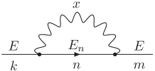
Figure 1: The Feynman diagram for the self-energy correction $\Sigma_{mk}$ in the one-loop order: the solid line stands for the spin and the wavy line stands for the bosonic freedom.

The actual evaluation of the Feynman diagram in Fig. 1 for the Ohmic case is straightforward by following the second-quantized formulation of the Caldeira-Leggett model 1992Fujikawa . The self-energy correction in the one-loop order is then given by (see Eq. (5) of 1992Fujikawa )

$$\Sigma_{mk}^{(1)} \equiv \eta\sum_{l=\pm}(w_{m}^{\dagger}{\sigma}_{z}w_{l})(w_{l}^{\dagger}\sigma_{z}w_{k})\Big{[}i(E-E_{l})\Theta(E-E_{l})$$ (20)

$$-\frac{(E_{l}-E)}{\pi}\ln\Big{|}\frac{\omega_{c}}{E-E_{l}}-1\Big{|}\Big{]},$$

in which $\Theta$ is the step function. The first term in Eq. (20), which is imaginary, gives the decay width of the $k$th level as

$$\frac{1}{2}\Gamma_{k}=\eta\sum_{l=\pm}\big{|}w_{k}^{\dagger}\sigma_{z}w_{l}\big{|}^{2}(E_{k}-E_{l})\Theta(E_{k}-E_{l}),$$ (21)

which vanishes for the ground state due to the step function. It indicates that the excited state decays to the ground state by emitting soft bosonic excitations. Below we will see that it characterizes the dephasing time scale of the spin system in magnetic field. The second term of Eq. (20) is a correction to the effective energy. As a result, the total effective energy, to the order of $O(\eta)$, becomes

$$E_{k}^{\text{tot}} = E_{k}+\frac{\eta}{\pi}\sum_{l=\pm}\big{|}w_{k}^{\dagger}\sigma_{z}w_{l}\big{|}^{2}(E_{l}-E_{k})$$ (22)

$$\times\ln\Big{|}\frac{\omega_{c}}{E_{k}-E_{l}}-1\Big{|}.$$

The Schrödinger amplitude in Eq. (17) to the accuracy of the lowest-order correction $O(\eta)$ is thus given by using Eqs.(21) and (22) as

$$\psi_{l}(t)\simeq e^{-\Gamma_{l}t/2}\exp[-i\int_{0}^{t}E_{l}^{\text{tot}}(t^{\prime})dt^{\prime}]w_{l}(t).$$ (23)

It appears that the probability conservation for the higher-energy state is violated in Eq. (23). Mathematically, this arises from the fact that we evaluated the “persistent” amplitude for the single-spin state under the influence of dissipation. Evolution operator (10) is formally unitary in the present case also. Thus the probability should be preserved in our formulation and also in the formulation with the density matrix in the Appendix.

In fact, the unitarity of the evolution operator, $U^{\dagger}(t)U(t)=1$, is preserved if one evaluates

$$w_{l_{+}}(t)\langle l_{+}|U(t)|l_{+}\rangle+w_{l_{-}}(t)\varphi_{B}(t)\langle l_{-};{\rm bosons}|U(t)|l_{+}\rangle,$$ (24)

since $w_{l_{-}}(t)\langle l_{-}|U(t)|l_{+}\rangle=0$ in the present model, where $\langle l_{\pm}|$ respectively stand for the higher- and lower-energy states of the spin, and $\langle l_{-};{\rm bosons}|$ stand for the final states of the lower energy spin state together with soft bosonic excitations. (To be more precise, one may write $\langle l_{\pm}|$ as $\langle l_{\pm}|\otimes\langle 0|$ and $\langle l_{-};{\rm bosons}|$ as $\langle l_{-}|\otimes\langle{\rm bosons}|$ with $\langle 0|$ standing for the bosonic vacuum. But we use the simplified notation in this paper.) Note that the description in terms of effective spectral density (19) is different from the description in terms of a definite number of bosonic quanta. In the spirit of the Caldeira-Leggett model 1981Caldeira , we do not assign a physical significance to the soft bosonic excitations footnote . In fact, the actual cause of the dissipation could be completely different from an ensemble of an infinite number of harmonic oscillators, though we consider that those harmonic oscillators, if suitably chosen, can mimic the actual dissipation. The presence of the dissipation is thus manifested by the decrease in the persistent amplitude $w_{l_{+}}(t)\langle l_{+}|U(t)|l_{+}\rangle$. [In this respect, our bosonic freedom is different from the time-component of the electromagnetic field in QED, which does not influence the unitarity. In path integral (18), one needs to add a Schwinger’s source term to the bosonic freedom also to analyze the unitarity.]

Since the final states $w_{l_{-}}(t)\varphi_{B}(t)\langle l_{-};{\rm bosons}|$ are orthogonal to both of $w_{l_{+}}(t)\langle l_{+}|$ and $w_{l_{-}}(t)\langle l_{-}|$ in Eq. (24) and thus do not interfere with these states when one considers only the observables of spin freedom as in the present case, the decrease in the persistent amplitude $w_{l_{+}}(t)\langle l_{+}|U(t)|l_{+}\rangle$ is also understood as an indicator of the quantum decoherence. See Eq. (28) in the Appendix. The inverse of the decay width in Eq. (21) is thus related to the two characteristic time scales of the qubits, namely, $\tau_{\text{relax}}$ and $\tau_{\varphi}$ 2008Clarke . The relaxation time scale $\tau_{\text{relax}}$ is the time required for a qubit to relax from the first excited state to the ground state, involving energy loss. The dephasing time scale $\tau_{\varphi}$ is the time over which the off-diagonal [in the preferred basis vectors $w_{\pm}(t)$] elements of the qubit’s reduced density matrix decay to zero in the formulation with the density matrix as in the Appendix. In the present model, these two time scales are of the same order of magnitude, and we choose $\tau_{\varphi}=2/\Gamma_{l{+}}$ by using the decay width in Eq. (21). We thus need to satisfy $T\ll\tau_{\varphi}$ or

$$\omega_{0}\gg\pi\Gamma_{l{+}},$$ (25)

to make a sensible measurement of geometric phases, which are defined for pure states. The gauge-invariant geometric phases for mixed states can be defined, but their measurement is generally rather indirect 2007Fujikawa .

III.1 Adiabatic Berry phase

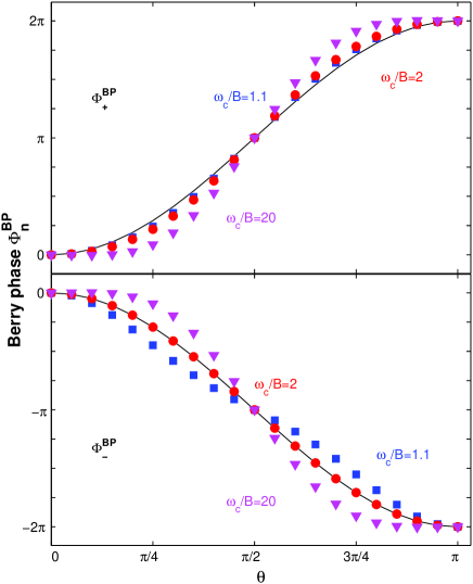
Figure 2: (Color online) Berry phase $\Phi_{n}^{\text{BP}}$ for various values of cutoff $\omega_{c}/B$. The black line corresponds to the dissipationless case, while marker points represent the case with dissipation. We set the dimensionless parameter $\eta=0.3$ and take ${\rm sign}(\omega_{0})=+1$. The values of the period $T=2\pi/\omega_{0}$ and the field strength $B/2\pi=50\times 10^{6}$(Hz) are taken from 2007Leek .

We now come to the analysis of GPs with dissipation. For definiteness, let us first analyze the environmental effects on the adiabatic BP. In the adiabatic limit $\theta_{0}\simeq\sin\theta\omega_{0}/B\rightarrow 0$ in Eq. (9), one has the non-vanishing quantities

$$\tau_{\varphi}^{-1} = \eta\sin^{2}\theta(B-\omega_{0}\cos\theta),$$

$$E_{\pm}^{\text{tot}} = \mp\frac{1}{2}B-\frac{1}{2}\omega_{0}(1\pm\cos\theta)\pm\frac{\eta}{\pi}\sin^{2}\theta(B$$

$$-\omega_{0}\cos\theta)\ln\Big{|}1\pm\frac{\omega_{c}}{B+\omega_{0}\cos\theta}\Big{|}.$$

Here we mention that to derive above $\tau_{\varphi}^{-1}$, we first set $\theta_{0}\simeq\sin\theta\omega_{0}/B$ and then let $\omega_{0}/B\rightarrow 0$ in formula (21). For $|\omega_{0}|\ll B<\omega_{c}$, the logarithm in the last term is nearly independent of geometry and its sign is very important because it determines whether the correction term is added or subtracted. After evolving one cycle $T$ ($2\pi/B\ll T\ll\tau_{\varphi}$), if one defines the phase $\Phi_{l}=\Phi_{l}^{\text{DP}}+\Phi_{l}^{\text{BP}}=\int_{0}^{T}E_{l}^{\text{tot}}(t)dt$ up to $2\pi n$ ($n=$integer), we may identify DP and BP respectively as

$$\Phi^{\text{DP}}_{\pm} = \mp\frac{1}{2}BT\pm\frac{\eta}{\pi}\sin^{2}\theta BT\ln\left|1\pm\frac{\omega_{c}}{B}\right|,$$

$$\Phi^{\text{BP}}_{\pm} = \mathrm{sgn}(\omega_{0})\left[\pm\Omega\mp 2\eta\sin^{2}\theta\cos\theta\ln\left|1\pm\frac{\omega_{c}}{B}\right|\right],$$

where the solid angle $\Omega=\pi(1-\cos\theta)$. The first terms in both DP and BP above are the ones in the absence of noise, while the second terms arise from the coupling between qubit and environment. Our results on the correction of BP and the geometric dephasing factor are consistent with those found by Whitney and co-workers 2003Whitney ; 2005Whitney .

If $\omega_{c}<2B$, the BP correction of the ground state would have the same sign as that of the excited state. Otherwise, the sign will be opposite. For an illustration, we plot $\Phi_{\pm}^{\text{BP}}$ with respect to the polar angle $\theta$ for various values of the cutoff $\omega_{c}/B$ in Fig. 2.

In passing, for a super-Ohmic case $J(\omega)=\eta\omega^{3}$ the dephasing time scale is given by $\tau_{\varphi}^{-1}=\eta\sin^{2}\theta B^{2}(B+\omega_{0}\cos\theta)$ and the correction to BP becomes $\Delta\Phi^{\text{BP}}_{\pm}=\mp{\rm sign}(\omega_{0})2\eta\sin^{2}\theta\cos\theta\left(\omega_{c}^{2}/2-B^{2}\ln|1\pm\omega_{c}/B|\right)$ in the adiabatic limit.

III.2 Nonadiabatic geometrical phase

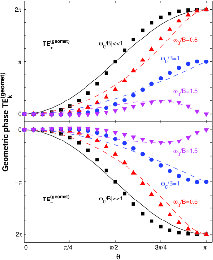
Figure 3: (Color online) Non-adiabatic geometric phases for different evolution rates $\omega_{0}/B$, in the presence or absence of environment. All lines including solid and dashed ones correspond to the nonadiabatic GPs without environment coupling (i.e., $\Omega_{k}$), while all marker points represent GPs, $TE_{k}^{(\text{geomet})}$, with environment coupling. The adiabatic limit of $|\omega_{0}/B|\ll 1$ is shown by black color. We set the dimensionless parameter $\eta=0.3$ and take ${\rm sign}(\omega_{0})=+1$. Other parameters are chosen as $B/2\pi=50\times 10^{6}$(Hz) and $\omega_{c}=3B$.

We emphasize that our formula (23) is valid for both of the adiabatic and nonadiabatic cases. Thus the modification of nonadiabatic (Aharonov-Anandan) GP due to the dissipation is analyzed quantitatively. A technical issue involved here is that a clear separation of dissipation-induced GP from dissipation-induced DP is not possible; One already recognizes this tendency even in the case without dissipation in Eq. (II). We here tentatively employ the following procedure for identifying the geometric phase away from the ideal adiabaticity with dissipation. As for the phase without dissipation, we adopt the separation in Eq. (II). For the phase induced by dissipation, we define the geometric part by

$$T\Delta E_{k}^{({\rm geomet})}=T[\Delta E_{k}(\omega_{0})-\Delta E_{k}(\omega_{0}=0)],$$

where $\Delta E_{k}(\omega_{0})$ stands for the second term in Eq. (22) proportional to $\eta$, and $T=2\pi/|\omega_{0}|$. This identification may be reasonable if both of $\omega_{0}$ and $\eta$ are small. Thus the total geometric phase is

$$TE_{k}^{({\rm geomet})}\equiv\Omega_{k}+T\Delta E_{k}^{({\rm geomet})},$$

which is illustrated in Fig. 3 with respect to the variable $\theta$. Here $\Omega_{k}=\pm\Omega_{\theta_{0}}$ stands for the nonadiabatic GP without dissipation obtained by multiplying the period $T$ to the second “geometric energy” in Eq. (II) and $\Omega_{\theta_{0}}=\pi[1-\cos(\theta-\theta_{0})]$ stands for the (nonadiabatic) solid angle with $\theta_{0}$ defined in Eq. (7). When taking the adiabatic limit of $|\omega_{0}/B|\ll 1$, $TE_{k}^{(\text{geomet})}$ approaches the adiabatic Berry phase with dissipation. When taking $\eta=0$, $TE_{k}^{(\text{geomet})}$ is reduced to the nonadiabatic GP $\Omega_{k}=\pm\Omega_{\theta_{0}}$ without dissipation.

Figure 3 illustrates how the observed GPs, with and without the effects of environment, deviate from the supposedly topological BP, $\pm\pi(1-\cos\theta)$, when the variables $\omega_{0}$ and $\eta$ deviate away from negligibly small values. It can be seen that the nonadiabatic GP is affected sensitively by the change in the dynamical parameter $\omega_{0}/B$, while the adiabatic BP is supposed to be immune to small fluctuations of $\omega_{0}/B$. This is related to the basic issue of the intrinsic robustness of BP. When $\omega_{0}/B$ becomes big (e.g., $>1$ in our choice of the parameter values), the non-monotonous magenta dashed lines localized near zero in Fig. 3 show that the dissipationless nonadiabatic GP $\Omega_{k}$ tends to be restricted in the neighborhood of zero, the trivial value of GP.

In the transitional region from adiabatic to nonadiabatic limit, the effect of environment on GP changes as $\theta$ increases and keeps the same pattern for diverse $\omega_{0}/B$, as indicated by the red and blue lines in Fig. 3. The red dashed lines, corresponding to a relatively small value of $\omega_{0}/B$, tends to recover the adiabatic case shown in Fig. 2, while the blue dashed lines away from both the adiabatic and nonadiabatic limits reflect the transitional region. One may note that at $\theta=\pi$ GP takes one of values of $0$, $\pm\pi$, and $\pm 2\pi$, which sharply depends on the value of $\omega_{0}/B$. This can be easily understood from the definition of $\theta_{0}$ in Eq. (7). In addition, it should be mentioned that for a fixed value of $\omega_{0}/B$ the $TE_{+}^{(\text{geomet})}$ and $TE_{-}^{(\text{geomet})}$ are not symmetric about the axis of $TE_{k}^{(\text{geomet})}=0$ due to the existence of the logarithmic term in Eq. (22). As for the role of the coupling strength $\eta$, it determines the magnitude of deviations, while having little effect on the pattern of deviations at least in the perturbative domain.

Finally, let us briefly analyze the geometric dephasing factor for the nonadiabatic case. From Eq. (21), the nonvanishing decay width is given by

$$\frac{1}{2}\Gamma_{-}=\eta\sin^{2}(\theta-\theta_{0})[B\cos\theta_{0}+\omega_{0}\cos(\theta-\theta_{0})].$$

Its geometric dependence is complicated because of the involvement of $\theta_{0}$ through Eq. (7). At the adiabatic limit, it returns to the $\tau_{\varphi}^{-1}$ discussed in Sec. III.1. At the nonadiabatic limit, we have $(\theta-\theta_{0})\sim 0$ and thus realize a dephasing-free situation. Unfortunately, the limit corresponds to the trivial geometric phase.

IV Conclusion

We have presented a gauge-invariant formulation of GPs for a two-level system in dissipative environment, which is applicable to both of adiabatic and nonadiabatic cases. Our formulation may be useful for understanding the experimental observation of BP such as in a recent superconducting qubit 2007Leek and will provide a starting point for the future quantitative analysis of the basic issues of intrinsic robustness 2003Blais and the behavior of GP in the transitional region away from ideal adiabaticity. The analysis of the region away from ideal adiabaticity is expected to be crucial in any practical application of geometric phases.

Appendix A Density matrix

One may be interested in the mixed states which are described by a density matrix in general. The time development of the density matrix $\rho$ is described by the evolution operator as

$$\rho(t)=U(t)\rho(0)U^{\dagger}(t),$$ (26)

at the vanishing temperature $T=0$. The evaluation of $U(t)$ is thus sufficient. For our purpose of simulating the dissipation by an infinite number of harmonic oscillators, one may trace out $\rho(t)=U(t)\rho(0)U^{\dagger}(t)$ with respect to all those final states which contain bosonic excitations. In our simple model, the bosonic excitations are included only in the lower-energy state of the fermion as in Eq. (24). If one defines a state

$$\psi(t)=a\psi_{l_{+}}(t)+b\psi_{l_{-}}(t),$$ (27)

with constants $a$ and $b$, which is no more cyclic even without dissipation since $\psi(T)\neq\psi(0)$ up to a phase, and starts with a pure state $\rho(0)=|\psi(0)\rangle\langle\psi(0)|$, one obtains the mixed state after partial tracing of $\rho(t)$ over those final bosonic excitations as

$$\tilde{\rho}(t) = |\psi(t)\rangle\langle\psi(t)|+|a|^{2}[|\psi_{l_{+}}(0)|^{2}-|\psi_{l_{+}}(t)|^{2}]\times$$ (28)

$$|\psi_{l_{-}}(t)\rangle\langle\psi_{l_{-}}(t)|,$$

with $|\psi_{l_{+}}(0)|^{2}=1$. We here used the unitarity relation in Eq. (24),

$$|\psi_{l_{+}}(t)|^{2}+\sum_{\rm bosons}|\langle{l_{-};\rm bosons}|U(t)|l_{+}\rangle|^{2}|\varphi_{B}(t)|^{2}|w_{l_{-}}(t)|^{2}$$

$$=|\psi_{l_{+}}(0)|^{2},$$ (29)

with $|w_{l_{-}}(t)|^{2}=1$. The first term in Eq. (28) arises from the trivial bosonic vacuum and the second term in Eq. (28) from the nontrivial bosonic states. The density matrix $\tilde{\rho}(t)$ approaches

$$\tilde{\rho}(t)\rightarrow(|a|^{2}+|b|^{2})|\psi_{l_{-}}(t)\rangle\langle\psi_{l_{-}}(t)|,$$ (30)

for $t\rightarrow{\rm large}$. Thus the total trace $\mathrm{Tr}\rho(t)=|a|^{2}+|b|^{2}$ is preserved during the time development in the present normalization of the density matrix.

One may define gauge invariant geometric phases for the mixed state described by this density matrix $\tilde{\rho}(t)$ following the general formulation in 2007Fujikawa . An interesting case is obtained if one sets $b=0$ and considers the time interval $t_{0}\leq t\leq t_{0}+T$ with $t_{0}\neq 0$ for $\tilde{\rho}(t)$.

References

- (1) J. Clarke and F. K. Wilhelm, Nature (London) 453, 1031 (2008).
- (2) J. Majer et al., Nature (London) 449, 443 (2007).
- (3) M. A. Sillanpää, J. I. Park, and R. W. Simmonds, Nature (London) 449, 438 (2007), and references therein.
- (4) Y. Makhlin, G. Schön, and A. Shnirman, Rev. Mod. Phys. 73, 357 (2001).
- (5) D. Vion et al., Science 296, 886 (2002).
- (6) M. V. Berry, Proc. R. Soc. London, Ser. A 392, 45 (1984).
- (7) J. Anandan, Nature (London) 360, 307 (1992).
- (8) P. J. Leek, et al., Science 318, 1889 (2007).
- (9) M. Möttönen, J. J. Vartiainen, and J. P. Pekola, Phys. Rev. Lett. 100, 177201 (2008).
- (10) Y. Nakamura, Yu. A. Pashkin, and J. S. Tsai, Nature (London) 398, 786 (1999).
- (11) P. Zanardi and M. Rasetti, Phys. Lett. A 264, 94 (1999).
- (12) A. Blais and A. M. S. Tremblay, Phys. Rev. A 67, 012308 (2003).
- (13) G. De Chiara and G. M. Palma, Phys. Rev. Lett. 91, 090404 (2003).
- (14) A. Carollo, I. Fuentes-Guridi, M. F. Santos, and V. Vedral, Phys. Rev. Lett. 90, 160402 (2003).
- (15) K.-P. Marzlin, S. Ghose, and B. C. Sanders, Phys. Rev. Lett. 93, 260402 (2004).
- (16) A. O. Caldeira and A. J. Leggett, Phys. Rev. Lett. 46, 211 (1981).
- (17) A. J. Leggett, et al., Rev. Mod. Phys. 59, 1 (1987).
- (18) R. S. Whitney and Y. Gefen, Phys. Rev. Lett. 90, 190402 (2003).
- (19) R. S. Whitney, Y. Makhlin, A. Shnirman, and Y. Gefen, Phys. Rev. Lett. 94, 070407 (2005).
- (20) Y. Aharonov and J. Anandan, Phys. Rev. Lett. 58, 1593 (1987).
- (21) J. Samuel and R. Bhandari, Phys. Rev. Lett. 60, 2339 (1988).
- (22) E. Farhi et al., Science 292, 472 (2001).
- (23) F. C. Lombardo and P. I. Villar, Phys. Rev. A 74, 042311 (2006).
- (24) S. Deguchi and K. Fujikawa, Phys. Rev. A 72, 012111 (2005).
- (25) K. Fujikawa, Phys. Rev. D 72, 025009 (2005).
- (26) K. Fujikawa, Ann. Phys. (N.Y.) 322, 1500 (2007).
- (27) K. Fujikawa, Phys. Rev. D 77, 045006 (2008).
- (28) B. Simon, Phys. Rev. Lett. 51, 2167 (1983).
- (29) K. Singh, D. M. Tong, K. Basu, J. L. Chen, and J. F. Du, Phys. Rev. A 67, 032106 (2003).
- (30) In the spirit of the Caldeira-Leggett model 1981Caldeira , we treat the bosonic freedom as an auxiliary device to simulate the dissipation. We do not take the infinite number of bosonic excitations as physical objects. See K. Fujikawa, Phys. Rev. E 57, 5023 (1998).
- (31) K. Fujikawa, S. Iso, M. Sasaki, and H. Suzuki, Phys. Rev. Lett. 68, 1093 (1992).