To what extent does genealogical ancestry imply genetic ancestry?

Abstract.

Recent statistical and computational analyses have shown that a genealogical most recent common ancestor (MRCA) may have lived in the recent past (Chang, 1999; Rohde et al., 2004). However, coalescent-based approaches show that genetic most recent common ancestors for a given non-recombining locus are typically much more ancient (Kingman, 1982a, b). It is not immediately clear how these two perspectives interact. This paper investigates relationships between the number of descendant alleles of an ancestor allele and the number of genealogical descendants of the individual who possessed that allele for a simple diploid genetic model extending the genealogical model of Chang (1999).

1. Introduction and model

Joseph Chang’s 1999 paper (Chang, 1999) showed that a well-mixed closed diploid population of $n$ individuals will have a genealogical common ancestor in the recent past. Specifically, the paper showed that if $T_{n}$ is the number of generations back to the most recent common ancestor (MRCA) of the population, then $T_{n}$ divided by $\log_{2}n$ converges to one in probability as $n$ goes to infinity. His paper initiated a discussion in which many of the leading figures of population genetics expressed interest in the relationship between the genealogical and genetic perspectives for such models (Donnelly et al., 1999). For example, Peter Donnelly wrote “[r]esults on the extent to which common ancestors, in the sense of [Chang’s] paper, are ancestors in the genetic sense… would also be of great interest” (Donnelly et al., 1999). Every other discussant also either discussed the relationship of Chang’s work to genetics or expressed interest in doing so.

Given this interest, surprisingly little work has been done specifically about the interplay between the two perspectives. Wiuf and Hein, in their reply, wrote three paragraphs containing some simple initial observations (Donnelly et al., 1999). Some simulation work has been done by Murphy (2004) with a more realistic population model. In a related though different vein, Möhle and Sagitov (2003) derived limiting results for the diploid coalescent, in the classical setting of a small sample from a large population.

In an interesting series of papers, Derrida, Manrubia, Zanette, and collaborators (Derrida et al., 1999, 2000a, 2000b; Manrubia et al., 2003) have investigated the distribution of the number of repetitions of ancestors in a genealogical tree, as well as the degree of concordance between the genealogical trees for two distinct individuals. Our paper, on the other hand, is concerned with correlations between the number of genealogical descendants of an individual and the number of descendant alleles of that individual. The interesting time-frame in our paper is different than theirs: they focus on the period substantially after $T_{n}$, while for us any interesting correlation is erased with high probability after time about $1.77T_{n}$.

Our paper attempts to connect the genealogical and genetic points of view by investigating several different questions concerning the interaction of genealogical ancestry and genetic ancestry in a diploid model incorporating Chang’s model. In classical Wright-Fisher fashion, we consider $2n$ alleles contained in $n$ diploid individuals. Each discrete generation forward in time, every individual selects two alleles from the previous generation independently and uniformly to “inherit.” If an individual $X$ at time $t$ inherits genetic information from an individual $Y$ at time $t-1$, then we consider $Y$ to be a “parent” of $X$ in the genealogical sense. As with Chang’s model, the two parents are permitted to be the same individual and each allele of a child may descend from the same parent allele. We illustrate the basic operation of the model in Figure 1. Each individual is represented as a circle, and each of a given individual’s alleles are represented as dots within the circle. Time increases down the figure and inheritance of alleles is represented by lines connecting them.

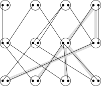
Figure 1. An example instance of our model with four individuals and three generations. Time increases moving down the diagram. The two alleles of each individual are depicted as two dots within the larger circles; a thin black line indicates genetic inheritance, i.e. the lower allele is descended from the upper allele. This sample genealogy demonstrates that the genealogical MRCA need not have any genetic relation to present-day individuals. The individual at the far right on the top row is in this case the (unique) MRCA as demonstrated by the thick gray lines, however none of its genetic material is passed onto the present day.

We have chosen notation in order to fit with Chang’s original article. The initial generation will be denoted $t=0$ and other generations will be counted forwards in time; thus the parents of the $t=1$ generation will be in the $t=0$ generation, and so on. The $n$ individuals of generation $t$ will be denoted $I_{t,1},\ldots,I_{t,n}$. The two alleles present at a given locus of individual $I_{t,i}$ will be labeled $A_{t,i,1}$ and $A_{t,i,2}$. Using this notation, each allele $A_{t,i,c}$ of generation $t$ selects an allele $A_{t-1,j,d}$ uniformly and independently from all of the alleles of the previous generation; given such a choice we say that allele $A_{t,i,c}$ is descended genetically from allele $A_{t-1,j,d}$. We define more distant ancestry recursively: allele $A_{t,i,c}$ is descended from allele $A_{t^{\prime},j,d}$ if $t>t^{\prime}$ and there exists a $k$ and $e$ such that allele $A_{t,i,c}$ is descended genetically from allele $A_{t-1,k,e}$ and allele $A_{t-1,k,e}$ is descended from or is the same as allele $A_{t^{\prime},j,d}$.

One can make a similar recursive definition of genealogical ancestry that matches Chang’s notion of ancestry: individual $I_{t,i}$ is descended genealogically from individual $I_{t^{\prime},j}$ if $t>t^{\prime}$ and there exists a $k$ such that individual $I_{t,i}$ is a parent of individual $I_{t-1,k}$ and individual $I_{t-1,k}$ is descended from or is the same as individual $I_{t^{\prime},j}$.

Define $\mathcal{Q}_{t}^{i}$ to be the alleles that are genetic descendants at time $t$ of the two alleles present in individual $I_{0,i}$, and let $Q_{t}^{i}$ be the number of such alleles. We will call the elements of $\mathcal{Q}_{t}^{i}$ the descendant alleles of individual $I_{0,i}$. Define $\mathcal{G}_{t}^{i}$ to be the genealogical descendants at time $t$ of the individual $I_{0,i}$, and let $G_{t}^{i}$ be the number of such individuals. We will say that a (genealogical) most recent common ancestor (MRCA) first appears at time $t$ if there is an individual $I_{0,i}$ in the population at time $0$ such that $G_{t}^{i}=n$ and $G_{s}^{j}<n$ for all $j$ and $s<t$; that is, individual $i$ in generation $0$ is a genealogical ancestor of all individuals in generation $t$, but there is no individual in generation $0$ that is a a genealogical ancestor of all individuals in any generation previous to generation $t$. Let $T_{n}$ denote the generation number at which the MRCA first appears. The main conclusion of Chang’s 1999 paper is that the ratio $T_{n}/\log_{2}n$ converges to one in probability as $n$ tends to infinity.

Our intent is to investigate the degree to which genealogical ancestry implies genetic ancestry. Unsurprisingly, historical individuals with more genealogical descendants will have more descendant alleles in expectation: in Proposition 1 we show that $\mathbb{E}[Q_{t}^{i}\,|\,G_{t}^{i}=k]$ is a super-linearly increasing function in $k$. However, in any realization of the stochastic process, individuals with more genealogical descendants need not have more descendant alleles. For example, in Figure 1 we show a case where the MRCA has no genetic relationship to any present day individuals. In the above notation, $G_{2}^{4}=n=4$ and yet $Q_{2}^{4}=0$.

Another approach is based on the rank of $G_{t}^{i}$. Loosely speaking, we are interested in the number of descendant alleles of the generation-$t$ individual with the $x$th most genealogical descendants. More rigorously, we consider the renumbering (opposite to the way rank is typically defined in statistics) $F(t,1),\ldots,F(t,n)$ of the indices $1,\ldots,n$ such that

$$G_{t}^{F(t,1)}\geq\cdots\geq G_{t}^{F(t,n)}$$

and if $G_{t}^{F(t,i)}=G_{t}^{F(t,j)}$ then fix $F(t,i)<F(t,j)$ when $i<j$. We then investigate $\left\{Q^{F(t,k)}:1\leq k\leq n\right\}$. These quantities give us concrete information about our main question in a relative sense: how much do individuals with many genealogical descendants contribute to the genetic makeup of present-day individuals compared to those with only a few? In Figure 2 we simulate our process 10000 times and then take an average for each time step, approximating $\mathbb{E}\left[Q_{t}^{F(t,k)}\right]$.

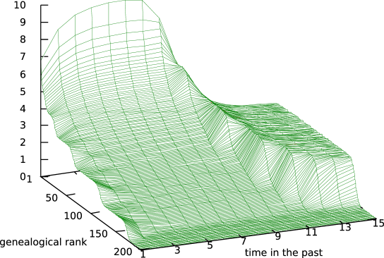
Figure 2. The expected number of descendant alleles from historical individuals sorted by number of genealogical descendants. Results by simulation of a population of size 200. For example, the value at “genealogical rank” 50 and time 2 is the expected number of alleles in the current population which descend from one or other of the two alleles present in the individual two generations ago who had no more genealogical descendants in the present population than did 49 other individuals in the population two generations ago. As described in the text, this curve attains an interesting characteristic shape around generation 3 that lasts until generation 8. We investigate that shape in Figure 3 and Proposition 2.

After several generations, the curve depicting $\mathbb{E}\left[Q_{t}^{F(t,k)}\right]$ acquires a characteristic shape which persists for some time, in this figure between time 3 and time 8. In order to explain what this curve is, we need to introduce some elementary facts about branching processes.

Recall that a branching process is a discrete time Markov process that tracks the population size of an idealized population (Athreya and Ney, 1972; Grimmett and Stirzaker, 2001). Each individual of generation $t$ produces an independent random number of offspring in generation $t+1$ according to some fixed probability distribution (the offspring distribution). This distribution is the same across all individuals. We will use the Poisson(2) branching process where the offspring distribution is Poisson with mean $2$ and write $B_{t}$ for the number of individuals in the $t^{\textrm{th}}$ generation starting with one individual at time $t=0$. It is a standard fact that the random variables $W_{t}=B_{t}/2^{t}$ converges almost surely as $t\rightarrow\infty$ to a random variable $W$ that is strictly positive on the event that the branching process doesn’t die out (that is, on the event that $B_{t}$ is strictly positive for all $t\geq 0$) – cf. Theorem 8.1 of (Athreya and Ney, 1972). Denote by $R$ the distribution of the limit random variable $W$. The probability measure $R$ is diffuse except for an atom at $0$ (that is, $0$ is the only point to which $R$ assigns non-zero mass). Also, the support of $R$ is the whole of $\mathbb{R}_{+}$ (that is, every open sub-interval of $\mathbb{R}_{+}$ is assigned strictly positive mass by $R$).

Returning to our discussion of $\mathbb{E}\left[Q_{t}^{F(t,k)}\right]$, define a non-increasing function $\gamma_{t,n}(c):(0,1)\rightarrow\mathbb{R}_{+}$ by

$$\gamma_{t,n}(c)=\mathbb{E}\left[Q_{t}^{F(t,\lfloor cn\rfloor})\right],$$

and define a non-increasing, continuous function $\beta:(0,1)\rightarrow\mathbb{R}_{+}$ by

(1) $$\begin{split}\beta(c)&=\min\{r\geq 0:R\left((r/2,\infty)\right)\leq c\}\\ &=\min\{r\geq 0:R\left([0,r/2]\right)\geq 1-c\}.\\ \end{split}$$

That is, $\beta(c)$ is the $(1-c)^{\mathrm{th}}$ quantile of $2W$, where the random variable $W$ is the limit of the normalized Poisson(2) branching process introduced above. Note that the function $\beta$ is strictly decreasing on the interval $(0,1-R(\{0\}))$; that is, $\beta(c)$ is the unique value $r$ for which $R((r/2,\infty))=c$ when $0<c<1-R(\{0\})$. We see experimentally that $\gamma_{6,200}$ is quite close to $\beta$ in Figure 3, and establish a convergence result in Proposition 2. Although a closed-form expression for the distribution $R$ is not available, there is a considerable amount known about this classical object (Van Mieghem, 2005). Note that the long-time behavior in Figure 2 is easily explained: it is simply the uniform distribution across only the common ancestors, that form $1-e^{-2}\simeq 0.864$ of the population.

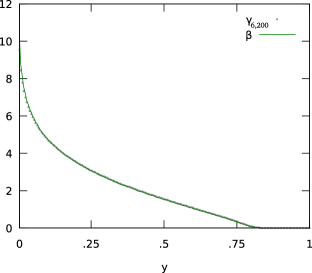
Figure 3. A plot of $\gamma_{6,200}$ and $\beta$, showing experimentally that the characteristic shape in Figure 2 is very close to the “tail-quantile” curve of a normalized Poisson(2) branching process. The curve for $\gamma_{6,200}$ was taken from Figure 2. To construct the curve for $\beta$, we wrote a subroutine that simulated 200 Poisson(2) branching processes simultaneously, then sorted the normalized results after 10 generations. This subroutine was run 10000 times and the average was taken. Note that the distribution had stabilized after 10 generations.

Thus far we have examined the connection between genealogical ancestry and genetic ancestry in the population as a whole; one may wonder about the number of descendants of the MRCA itself. Unfortunately, the story there is not as simple as could be desired. For example, there are usually multiple MRCAs appearing (by definition) in the same generation, and the expected number depends on $n$ in a surprising way (see Figure 4). We investigate this genealogical issue and related genetic questions in Section 4.

2. Monotonicity of the number of descendant alleles in terms of genealogy

In this section we prove the following result.

Proposition 1.

For each time $t\geq 2$, the function $k\mapsto k^{-1}\,\mathbb{E}[Q_{t}^{i}\,|\,G_{t}^{i}=k]$, $0\leq k\leq n$, is strictly increasing.

The key observation in the proof of Proposition 1 will be that the random variables $G_{t}^{i}$ and $G_{t+1}^{i}$ enjoy the property of total positivity investigated extensively in the statistical literature following Karlin (1968) (see, for example, (Brown et al., 1981)).

Definition 1.

A pair of random variables $(X,Y)$ has a strict TP(2) joint distribution if

$$\mathbb{P}\left\{X=x,Y=y\right\}\mathbb{P}\left\{X=x^{\prime},Y=y^{\prime}\right\}>\mathbb{P}\left\{X=x,Y=y^{\prime}\right\}\mathbb{P}\left\{X=x^{\prime},Y=y\right\}$$

for all $x<x^{\prime}$ and $y<y^{\prime}$ such that the left-hand side is strictly positive.

The proof of the next result is clear.

Lemma 1.

The following are equivalent to strict TP(2) for $x<x^{\prime}$ and $y<y^{\prime}$:

(2) $$\frac{\mathbb{P}\left\{Y=y^{\prime}\,|\,X=x^{\prime}\right\}}{\mathbb{P}\left\{Y=y^{\prime}\,|\,X=x\right\}} >\frac{\mathbb{P}\left\{Y=y\,|\,X=x^{\prime}\right\}}{\mathbb{P}\left\{Y=y\,|\,X=x\right\}}$$

(3) $$\frac{\mathbb{P}\left\{X=x^{\prime}|Y=y^{\prime}\right\}}{\mathbb{P}\left\{X=x^{\prime}\,|\,Y=y\right\}} >\frac{\mathbb{P}\left\{X=x|Y=y^{\prime}\right\}}{\mathbb{P}\left\{X=x\,|\,Y=y\right\}}.$$

Lemma 2.

The pair $(G_{t}^{i},G_{t+1}^{i})$ has a strict TP(2) joint distribution.

Proof.

We will show condition (2). By definition of our model, the number of genealogical descendants in generation $t+1$ has a conditional binomial distribution as follows:

$$\mathbb{P}\{G_{t+1}^{i}=k\,|\,G_{t}^{i}=r\}=\binom{n}{k}\left(2r/n-(r/n)^{2}\right)^{k}\left(1-2r/n+(r/n)^{2}\right)^{n-k}.$$

Set $x(r)=2r/n-(r/n)^{2}$, a function that is strictly increasing in $r$ for $0\leq r\leq n$. Then

$$\frac{\mathbb{P}\{G_{t+1}^{i}=k+1\,|\,G_{t}^{i}=r\}}{\mathbb{P}\{G_{t+1}^{i}=k\,|\,G_{t}^{i}=r\}}=\frac{n-k}{k+1}\cdot\frac{x(r)}{1-x(r)},$$

a function that is a strictly increasing function of $r$ for $1\leq r\leq n$. ∎

The following definition is well known to statisticians (Lehmann, 1986).

Definition 2.

Consider a reference measure $\mu$ on some space $\mathcal{X}$ and a parameterized family $\{p_{\theta}:\theta\in\Theta\}$ of probability densities with respect to $\mu$, where $\Theta$ is a subset of $\mathbb{R}$. Let $T$ be a real-valued function defined on $\mathcal{X}$. The family of densities has the monotone likelihood ratio property in $T$ with respect to the parameter $\theta$ if for any $\theta^{\prime}<\theta^{\prime\prime}$ the densities $p_{\theta^{\prime}}$ and $p_{\theta^{\prime\prime}}$ are distinct and $x\mapsto p_{\theta^{\prime\prime}}(x)/p_{\theta^{\prime}}(x)$ is a nondecreasing function of $T(x)$.

Lemma 3.

Fix a time $t\geq 0$. If the function $f:\mathbb{R}\rightarrow\mathbb{R}$ is strictly increasing, then the function $k\mapsto\mathbb{E}[f(G_{t}^{i})\,|\,G_{t+1}^{i}=k]$, $1\leq k\leq n$, is strictly increasing.

Proof.

By Lemma 2 and inequality (3), the family of probability densities (with respect to counting measure) $\mathbb{P}\left\{G_{t}^{i}=r\,|\,G_{t+1}^{i}=k\right\}$ parameterized by $k$ has monotone likelihood ratios in $r$ with respect to $k$. Now apply Lemma 2(i) of (Lehmann, 1986). ∎

Proof of Proposition 1.

For $t\geq 1$, let $\alpha_{t}(k)=k^{-1}\,\mathbb{E}[Q_{t}^{i}\,|\,G_{t}^{i}=k]$.

First note that each individual of $\mathcal{G}_{1}^{i}$ has a $1/n$ chance of choosing $I_{0,i}$ as a parent twice, thus

$$\alpha_{1}(k)=(1+1/n).$$

The result will thus follow by induction on $t$ if we can show for $t\geq 1$ that the function $k\mapsto\alpha_{t+1}(k)$ is strictly increasing whenever the function $k\mapsto\alpha_{t}(k)$ is non-decreasing. Therefore, fix $t\geq 1$ and suppose that the function $k\mapsto\alpha_{t}(k)$ is non-decreasing.

We first claim that

(4) $$k^{-1}\,\mathbb{E}[Q_{t+1}^{i}\,|\,G_{t}^{i}=r,\,G_{t+1}^{i}=k]=(r^{-1}+n^{-1})\,\mathbb{E}[Q_{t}^{i}\,|\,G_{t}^{i}=r]=f(r),$$

where

$$f(r)=\left(r^{-1}+n^{-1}\right)\mathbb{E}[Q_{t}^{i}\,|\,G_{t}^{i}=r]=\left(1+\frac{r}{n}\right)\alpha_{t}(r).$$

The proof of this claim is as follows.

Recall that $\mathcal{G}_{t}^{i}$ is the set of generation $t$ individuals descended from $I_{0,i}$, so that $\mathcal{G}_{t}^{i}$ has $G_{t}^{i}$ elements. Suppose that $G_{t}^{i}=r$ and number the elements of $\mathcal{G}_{t}^{i}$ as $1,\cdots,r$. Let $V_{j,c}$ be the indicator random variable for the event that the allele $A_{t,j,c}$ is descended from one of the alleles of $I_{0,i}$ for $1\leq j\leq r$. By definition, the sum of the $V_{j,c}$ is equal to $Q_{t}^{i}$. Note that any individual in $\mathcal{G}_{t+1}^{i}$ has one parent uniformly selected from $\mathcal{G}_{t}^{i}$ and the other uniformly selected from the population as a whole. Selections for different individuals are independent. Therefore,

$$\mathbb{E}[Q_{t+1}^{i}\,|\,G_{t}^{i}=r,\, G_{t+1}^{i}=k,V_{1,1},V_{1,2},\ldots,V_{r,1},V_{r,2}]$$

$$=k\left[\frac{1}{r}\sum_{\ell=1}^{r}(V_{\ell,1}+V_{\ell,2})+\frac{1}{n}\left(\sum_{\ell=1}^{r}(V_{\ell,1}+V_{\ell,2})+\sum_{\ell=r+1}^{n}0\right)\right]$$

$$=k(r^{-1}+n^{-1})Q_{t}^{i}$$

By the tower property of conditional expectation,

$$\mathbb{E}[Q_{t+1}^{i}\,|\,G_{t}^{i}=r,\,G_{t+1}^{i}=k]=k(r^{-1}+n^{-1})\mathbb{E}[Q_{t}^{i}\,|\,G_{t}^{i}=r,\,G_{t+1}^{i}=k].$$

An application of the Markov property now establishes our claim (4). Thus

$$\begin{split}k^{-1}\,\mathbb{E}[Q_{t+1}^{i}\,|\,G_{t+1}^{i}=k]&=\sum_{r=1}^{n}k^{-1}\,\mathbb{E}[Q_{t+1}^{i}\,|\,G_{t}^{i}=r,G_{t+1}^{i}=k]\,\mathbb{P}\{G_{t}^{i}=r\,|\,G_{t+1}^{i}=k\}\\ &=\sum_{r=1}^{n}\,f(r)\,\mathbb{P}\{G_{t}^{i}=r\,|\,G_{t+1}^{i}=k\}\\ &=\mathbb{E}[f(G_{t}^{i})\,|\,G_{t+1}^{i}=k].\\ \end{split}$$

This is strictly increasing in $k$ by Lemma 3 and the observation that $f$ is strictly increasing. ∎

3. The mysterious shape in Figure 2

In this section we investigate the shape of the curve relating the number of descendant alleles to genealogical rank. As shown in Figure 2, this curve attains a characteristic shape after several generations; the shape is maintained for a period prior to the time when the genealogical MRCA appears. We show that this curve is essentially the limiting “tail-quantile” of a normalized Poisson(2) branching process.

An important component of our analysis will be a multigraph representing ancestry that we will call the genealogy. A multigraph is similar to a graph except that multiple edges between pairs of nodes are allowed. Specifically, a multigraph is an ordered pair $(V,E)$ where $V$ is a set of nodes and $E$ is a multiset of unordered pairs of nodes.

Definition 3.

Define the time $t$ ancestry multigraph $\mathfrak{G}_{t}$ as follows. The nodes of this multigraph are the set of all individuals of generations zero through $t$; for any $0<t^{\prime}\leq t$ connect an $I_{t^{\prime},k}$ to $I_{t^{\prime}-1,j}$ if $I_{t^{\prime},k}$ is descended from $I_{t^{\prime}-1,j}$. If both parents of $I_{t^{\prime},k}$ are $I_{t^{\prime}-1,j}$, then add an additional edge connecting $I_{t^{\prime},k}$ and $I_{t^{\prime}-1,j}$. Define the time $t$ genealogy $\mathfrak{G}_{t}^{i}$ to be the subgraph of $\mathfrak{G}_{t}$ consisting of $I_{0,i}$ and all of its descendants $\bigcup_{t^{\prime}=0}^{t}\mathcal{G}_{t^{\prime}}^{i}$ up to time $t$.

Definition 4.

We define an ancestry path in $\mathfrak{G}_{t}^{i}$ to be a sequence of individuals $I_{0,i(0)},I_{1,i(1)},\cdots,I_{t,i(t)}$ with $i(0)=i$ where for each $0<t^{\prime}\leq t$, $I_{t^{\prime}-1,i(t^{\prime}-1)}$ is a parent of $I_{t^{\prime},i(t^{\prime})}$. Let $P_{t}^{i}$ be the number of ancestry paths in $\mathfrak{G}_{t}^{i}$.

We emphasize that a parent being selected twice by a single individual results in a “doubled” edge; paths that differ only in their choice of what edge to traverse between parent to child are considered distinct. Thus, each such doubled edge doubles the number of ancestry paths that contain the corresponding parent-child pair.

Our result concerning the connection between the curve in Figure 2 and the Poisson(2) branching process can be stated as follows. Define a random probability measure on the positive quadrant that puts mass $1/n$ at each of the points $(\mathbb{E}[Q_{t}^{i}\,|\,\mathfrak{G}_{t}],2^{1-t}G_{t}^{i})$. We show below that this random probability measure converges in probability to a deterministic probability measure concentrated on the diagonal and has projections onto either axis given by the limiting distribution of $2^{1-t}B_{t}$ as $t\rightarrow\infty$.

We may describe the convergence more concretely by using the idea of “sorting by the number of genealogical descendants” as in the introduction; using the notation introduced there, let the random variable $F(t,k)$ denote the index of the individual in generation $0$ with the $k^{\mathrm{th}}$ greatest number of genealogical descendants at time $t$. Recall the non-increasing, continuous function $\beta:(0,1)\rightarrow\mathbb{R}_{+}$ defined in equation (1).

Proposition 2.

Suppose that $0<a<b<1-R(\{0\})$, so that $\infty>\beta(a)>\beta(b)>0$. Then

$$\frac{1}{n(b-a)}\cdot\#\left\{an\leq k\leq bn:\mathbb{E}\left[\left.Q_{t}^{F(t,k)}\right|\mathfrak{G}_{t}\right]\in[\beta(b),\beta(a)]\right\}$$

converges to $1$ in probability as $t=t_{n}$ and $n$ go to infinity in such a way that $2^{2t_{n}}/n\rightarrow 0$.

Note that the condition $2^{2t_{n}}/n\rightarrow 0$ is satisfied, for example, when $t_{n}=\tau\log_{2}n$ for $\tau<1/2$.

The proof of Proposition 2 formalizes the following three common-sense notions about the ancestry process.

Note that for $t>1$, the genealogy will not necessarily be a tree: it may be possible to follow two different ancestry paths through $\mathfrak{G}_{t}^{i}$ to a given time-$t$ individual. However, our first intuition is that this possibility is rare when $n$ is large and $t$ is small relative to $n$, and such events do not affect the values of $G_{t}^{i}$ and $Q_{t}^{i}$ in the limit.

Second, the fact that each of the above genealogies is usually a tree suggests that we may be able to relate the ancestry process to a branching process. In our case, the number of immediate descendants for an individual $I_{t^{\prime}-1,j}$ is the number of times a individual of generation $t^{\prime}$ chooses $I_{t^{\prime}-1,j}$ as a parent. These numbers are not exactly independent: for example, if all of the individuals of generation $t^{\prime}$ descend only from a single individual of generation $t^{\prime}-1$, then the number of descendants of the other individuals is exactly zero. However, we will show that these numbers are close to independent when $n$ becomes large. Also, note that the marginal distribution of the number of next-generation descendants of a single individual is binomial: there are $2n$ trials each with probability $1/n$. As $n$ goes to infinity, this is approximately a Poisson(2) random variable. In summary, we will show that the genealogy of an individual is close to that of a Poisson(2) branching process for short times relative to the population size.

Third, we note that there is a simple relationship between the number of paths $P_{t}^{i}$ and the expected number of descendant alleles $Q_{t}^{i}$:

Lemma 4.

$\mathbb{E}\left[Q_{t}^{i}\,|\,\mathfrak{G}_{t}^{i}\right]=2^{1-t}P_{t}^{i}$.

Proof.

Consider an arbitrary path in the ancestry graph $\mathfrak{G}_{t}^{i}$ and pick an arbitrary edge in that path. Suppose the edge connects $I_{t^{\prime}-1,j}$ to $I_{t^{\prime},i}$. By the definition of the model, $I_{t^{\prime},i}$ has probability $1/2$ of inheriting any fixed allele of $I_{t^{\prime}-1,j}$. Thus, the contribution of any single allele of $I_{0,i}$ and given path in $\mathfrak{G}_{t}^{i}$ to the expectation of $Q_{t}^{i}$ is $2^{-t}$. The contribution of both alleles of $I_{0,i}$ is $2^{1-t}$. The total number of alleles descended from the alleles of $I_{0,i}$ is the sum over the contributions of all paths, and the expectation of this sum is the sum of the expectations. ∎

We will use the probabilistic method of coupling to formalize the connection between the genealogical process and the branching process. A coupling of random variables $X$ and $Y$ that are not necessarily defined on the same probability space is a pair of random variables $X^{\prime}$ and $Y^{\prime}$ defined on a single probability space such that the marginal distributions of $X$ and $X^{\prime}$ (respectively, $Y^{\prime}$ and $Y$) are the same. A simple example of coupling is “Poisson thinning”, a coupling between an $X\sim\mathrm{Poisson}(\lambda_{1})$ and a $Y\sim\mathrm{Poisson}(\lambda_{2})$ where $\lambda_{1}\geq\lambda_{2}$. To construct the pair $(X^{\prime},Y^{\prime})$, one first gains a sample for $X^{\prime}$ by simply sampling from $X$. The sample from $Y^{\prime}$ is then gained by “throwing away” points from the sample for $X^{\prime}$ with probability $\lambda_{2}/\lambda_{1}$; i.e. the distribution for $Y^{\prime}$ conditioned on the value $x$ for $X^{\prime}$ is just $\operatorname{Binomial}(x,1-\lambda_{2}/\lambda_{1}).$

We note that coupling is a popular tool for questions with a flavour similar to ours. Recently Barbour (2007) has coupled an epidemics model to a branching process and Durrett et al. (2007) have used coupling to analyze a model of carcinogenesis.

Recall that we defined $W_{t}=B_{t}/2^{t}$, where $B_{t}$ is a Poisson(2) branching processes started at time $t=0$ from a single individual, and we observed that the sequence of random variables $W_{t}$ converges almost surely to a random variable $W$ with distribution $R$. The following lemma is the coupling result that will give the convergence of the sampling distribution of the $P_{t}^{i}$ and $G_{t}^{i}$ to $R$ in Lemma 6 below.

Lemma 5.

There is a coupling between $P_{t}^{i}$, $G_{t}^{i}$, and $B_{t}^{i}$, where $B_{t}^{1},B_{t}^{2},\ldots$ is a sequence of independent Poisson(2) branching processes, such that for a fixed positive integer $\ell$ the probability

$$\mathbb{P}\{P_{t}^{i}=G_{t}^{i}=B_{t}^{i},\,1\leq i\leq\ell\}$$

converges to one as $n$ goes to infinity with $t=t_{n}$ satisfying $2^{2t_{n}}/n\rightarrow 0$.

Proof.

We introduce the coupling between the ancestral process and the branching process by looking first at the transition from generation $0$ to generation $1$. Suppose that we designate a set $S$ of $k$ individuals in generation $0$ and write $G$ for the number of descendants these $k$ individuals have in generation $1$.

The probability that there is an individual in generation $1$ who picks both of its parents from the $k$ designated individuals is

$$1-\left(1-\left(k/n\right)^{2}\right)^{n}\leq k^{2}/n.$$

Couple the random variable $G$ with a random variable $P$ that is the same as $G$ except that we (potentially repeatedly) re-sample any generation $1$ individual who chooses two parents from $S$ until it has at least one parent not belonging to $S$. The random variable $P$ will have a binomial distribution with number of trials $n$ and success probability

(5) $$\frac{2\frac{k}{n}\left(1-\frac{k}{n}\right)}{1-\frac{k^{2}}{n^{2}}}=\frac{2\frac{k}{n}}{1+\frac{k}{n}},$$

which is simply the probability of an individual selecting exactly one parent from the set of $k$ given that it does not select two. By the above,

$$\mathbb{P}\{G\neq P\}\leq\frac{k^{2}}{n}.$$

By a special case of Le Cam’s Poisson approximation result (Grimmett and Stirzaker, 2001; Le Cam, 1960), we can couple the random variable $P$ to a random variable $Y$ that is Poisson distributed with mean

$$n\frac{2\frac{k}{n}}{1+\frac{k}{n}}=\frac{2k}{1+\frac{k}{n}}$$

in such a way that

$$\mathbb{P}\{P\neq Y\}\leq n\left(\frac{2\frac{k}{n}}{1+\frac{k}{n}}\right)^{2}\leq 4\frac{k^{2}}{n}.$$

Moreover, a straightforward argument using Poisson thinning shows that we can couple the random variable $Y$ with a random variable $B$ that is Poisson distributed with mean $2k$ such that

$$\mathbb{P}\{Y\neq B\}\leq\left|2k-\frac{2k}{1+\frac{k}{n}}\right|\leq 2\frac{k^{2}}{n}.$$

Putting this all together, we see that we can couple the random variables $G$, $P$, and $B$ together in such a way that

$$\mathbb{P}(\neg\{G=P=B\})\leq 8\frac{k^{2}}{n}$$

where $\neg$ denotes complement. Note that $B$ may be thought of as the sum of $k$ independent random variables, each having a Poisson distribution with mean $2$.

Fix an index $i$ with $1\leq i\leq n$. Returning to the notation used in the rest of the paper, the above triple $(G,P,B)$ correspond to $(G_{t}^{i},P_{t}^{i},B_{t}^{i})$, and $k$ plays the role of $G_{t-1}^{i}$. Now suppose we start with one designated individual $i$ in the population at generation $0$. Let $S_{t}$ denote the event

$$\{P_{t}^{i}=G_{t}^{i}=B_{t}^{i}\}.$$

The above argument shows that we can couple the process $P^{i}$ with the branching process $B^{i}$ in such a way that

$$\begin{split}\mathbb{P}\{\neg S_{t}\}&\leq\mathbb{P}\{\neg S_{t-1}\}+\mathbb{P}\{\neg S_{t},\;S_{t-1}\}\\ &\leq\mathbb{P}\{\neg S_{t-1}\}+\mathbb{E}\left[8\frac{B_{t-1}^{2}}{n}\right]\\ &\leq\mathbb{E}\{\neg S_{t-1}\}+\frac{c2^{2(t-1)}}{n}\\ \end{split}$$

for a suitable constant $c$ (using standard formulae for moments of branching processes). Iterating this bound gives

$$\mathbb{P}\{\neg S_{t}\}\leq\frac{c^{\prime}2^{2t}}{n}$$

for a suitable constant $c^{\prime}$.

This tells us that when $n$ is large, the random variable $P_{t}^{i}$ is close to the random variable $B_{t}^{i}$ not just for fixed times but more generally for times $t$ such that $2^{2t}/n\rightarrow 0$. As mentioned above, this condition is satisfied when $t=\tau\log_{2}n$ for $\tau<1/2$.

Next, we elaborate the above argument to handle the descendants of $\ell$ individuals. Let $S_{t}^{\ell}$ denote the event that the $\ell$ coupled triples of random variables are equal, that is,

$$\{P_{t}^{1}=G_{t}^{1}=B_{t}^{1},\,P_{t}^{2}=G_{t}^{2}=B_{t}^{2},\ldots,P_{t}^{\ell}=G_{t}^{\ell}=B_{t}^{\ell}\},$$

where $B_{t}^{i}$ is the branching process coupled to $P_{t}^{i}$ and $G_{t}^{i}$. By mimicking the above argument, we can show that

$$\mathbb{P}\{\neg S_{t}^{\ell}\}\leq\mathbb{P}\{\neg S_{t-1}^{\ell}\}+c\ell\,2^{2(t-1)}/n.$$

Again, iterating this bound gets

$$\mathbb{P}\{\neg S_{t}^{\ell}\}\leq c^{\prime}\ell\,2^{2t}/n$$

for some $c^{\prime}$. ∎

For any Borel subset $C$ of $\mathbb{R}_{+}^{2}$, let $\eta_{t,n}(C)$ denote the joint empirical distribution of the normalized $P_{t}^{i}$ and the normalized $G_{t}^{i}$ at time $t$, i.e.

$$\eta_{t,n}(C)=\frac{1}{n}\cdot\#\{1\leq i\leq n:(2^{-t}P_{t}^{i},2^{-t}G_{t}^{i})\in C\}.$$

In Lemma 6 we demonstrate that the $\eta_{t,n}$ converge in probability to the deterministic probability measure $\eta(dx,dy)=R(dx)\delta_{x}(dy)=\delta_{y}(dx)R(dy)$ concentrated on the diagonal, where $\delta_{z}$ denotes the unit point mass at $z$.

The mode of convergence may require a bit of explanation. When we say that a real-valued random variable converges in probability to a fixed quantity, there is an implicit and commonly understood notion of convergence of a sequence of real numbers. However, here the random quantities are probability measures, and the underlying notion we use for convergence of measures is that of weak convergence. Recall that a sequence of probability measures $\mu_{n}$ on $\mathbb{R}_{+}^{2}$ is said to converge to $\mu$ weakly if $\int f\,d\mu_{n}$ converges to $\int f\,d\mu$ for all bounded continuous functions $f:\mathbb{R}_{+}^{2}\rightarrow\mathbb{R}$. The following are equivalent conditions for sequence of probability measures $\mu_{n}$ to converge to $\mu$ weakly: (i) $\limsup_{n}\mu_{n}(F)\leq\mu(F)$ for all closed sets $F\subseteq\mathbb{R}_{+}^{2}$, (ii) $\liminf_{n}\mu_{n}(G)\geq\mu(G)$ for all open sets $G\subseteq\mathbb{R}_{+}^{2}$, (iii) $\lim_{n}\mu_{n}(A)=\mu(A)$ for all Borel sets $A\subseteq\mathbb{R}_{+}^{2}$ such that $\mu(\partial A)=0$, where $\partial A$ is the boundary of $A$.

Lemma 6.

Suppose that $t=t_{n}$ converges to infinity as n goes to infinity in such a way that $\lim_{n\rightarrow\infty}2^{2t_{n}}/n\rightarrow 0$. Then the sequence of random measures $\eta_{t,n}$ converges in probability as $n\rightarrow\infty$ to the deterministic probability measure $\eta$ on $\mathbb{R}_{+}^{2}$ that assigns mass $R(A\cap B)$ to sets of the form $A\times B$.

Proof.

For brevity, let $H_{t}^{i}$ denote the pair $(2^{-t}P_{t}^{i},2^{-t}G_{t}^{i})$. Fix a bounded continuous function $f:\mathbb{R}_{+}^{2}\rightarrow\mathbb{R}$. By definition,

$$\begin{split}\mathbb{E}\left[\left(\int f\,d\eta_{t,n}\right)^{2}\right]\\ &=n^{-2}\,\mathbb{E}\left[\sum_{i}f^{2}(H_{t}^{i})+\sum_{i\neq j}f(H_{t}^{i})f(H_{t}^{j})\right]\\ &=n^{-2}\left(n\mathbb{E}[f^{2}(H_{t}^{1})]+n(n-1)\mathbb{E}[f(H_{t}^{1})f(H_{t}^{2})]\right).\\ \end{split}$$

Hence, $\mathbb{E}[(\int f\,d\eta_{t,n})^{2}]$ is asymptotically equivalent to

(6) $$\mathbb{E}[f(H_{t}^{1})f(H_{t}^{2})].$$

By definition, (6) is equal to

(7) $$\mathbb{E}[f(2^{-t}P_{t}^{1},2^{-t}G_{t}^{1})\,f(2^{-t}P_{t}^{2},2^{-t}G_{t}^{2})].$$

Lemma 5 establishes a coupling such that $P_{t}^{i}=G_{t}^{i}=B_{t}^{i}$ with probability tending to one in the limit under our hypotheses. Thus, under our conditions on $t=t_{n}$ the expectation (7), and hence $\mathbb{E}[(\int f\,d\eta_{t,n})^{2}]$, converges to

$$\begin{split}\lim_{t\rightarrow\infty}\mathbb{E}[f(W_{t}^{1})f(W_{t}^{2})]&=\lim_{t\rightarrow\infty}\mathbb{E}[f(W_{t}^{1},W_{t}^{1})]\mathbb{E}[f(W_{t}^{2},W_{t}^{2})]\\ &=\left(\int_{\mathbb{R}_{+}}f(x,x)\,R(dx)\right)^{2}\\ &=\left(\int_{\mathbb{R}_{+}^{2}}f\,d\eta\right)^{2}.\\ \end{split}$$

A similar but simpler argument shows that $\mathbb{E}[\int f\,d\eta_{t,n}]$ converges to $\int f\,d\eta$. Combining these two facts shows that $\operatorname{Var}[\int f\,d\eta_{t,n}]$ converges to zero.

Therefore, $\int f\,d\eta_{t,n}$ converges in probability to $\int f\,d\eta$ for all bounded continuous functions $f$, as required. ∎

Proof of Proposition 2.

It suffices by Lemma 4 to show that

$$\frac{1}{n(b-a)}\cdot\#\left\{an\leq k\leq bn:2^{-t}P_{t}^{F(t,k)}\in[2\beta(b),2\beta(a)]\right\}$$

converges to $1$ in probability as $t=t_{n}$ and $n$ go to infinity in such a way that $2^{2t_{n}}/n\rightarrow 0$.

For $\gamma>0$ and an integer $1\leq k\leq n$,

$$\begin{split}&\eta_{t,n}(\mathbb{R}_{+}\times[\gamma,\infty))\geq\frac{k}{n}\\ &\quad\Leftrightarrow\#\{1\leq i\leq n:2^{-t}G_{t}^{i}\geq\gamma\}\geq k\\ &\quad\Leftrightarrow 2^{-t}G_{t}^{F(t,k)}\geq\gamma,\\ \end{split}$$

by definition of the empirical distribution $\eta_{t,n}$ and the indices $F(t,k)$. Because the limit measure $\eta$ assigns zero mass to the boundary $\mathbb{R}_{+}\times\{\gamma\}$ of the set $\mathbb{R}_{+}\times[\gamma,\infty)$, it follows from Lemma 6 that

$$\frac{1}{n}\cdot\#\{1\leq i\leq n:2^{-t}G_{t}^{i}\geq\gamma\}$$

converges to $\eta(\mathbb{R}_{+}\times[\gamma,\infty))=R([\gamma,\infty))$ in probability. In particular,

$$\frac{1}{n}\cdot\#\{1\leq i\leq n:2^{-t}G_{t}^{i}\geq 2\beta(c)\}$$

converges to $c$ in probability for $0<c<1-R(\{0\})$. Thus, $2^{-t}G_{t}^{F(t,\lfloor cn\rfloor)}$ converges in probability to $2\beta(c)$ for such a $c$.

With $0<a<b<1-R(\{0\})$ as in the statement of the proposition, it follows that

$$\frac{1}{n}\cdot\#\left\{an\leq k\leq bn:2^{-t}G_{t}^{F(t,k)}\in[2\beta(b-\epsilon),2\beta(a+\epsilon)]\right\}$$

converges in probability to $(b-a-2\epsilon)$ for $0<\epsilon<(b-a)/2$.

Note by Lemma 6 that

$$\begin{split}&\frac{1}{n}\cdot\#\left\{1\leq k\leq n:\left|2^{-t}P_{t}^{F(t,k)}-2^{-t}G_{t}^{F(t,k)}\right|>\delta\right\}\\ &\quad=\eta_{t,n}(\{(x,y)\in\mathbb{R}_{+}^{2}:|x-y|>\delta\})\\ \end{split}$$

converges in probability to $0$ for any $\delta>0$, because the probability measure $\eta$ assigns all of its mass to the diagonal $\{(x,y)\in\mathbb{R}_{+}^{2}:x=y\}$.

Taking $\delta<2\min\{\beta(a)-\beta(a+\epsilon),\beta(b-\epsilon)-\beta(b)\}$ so that

$$[2\beta(b-\varepsilon)-\delta,2\beta(a+\varepsilon)+\delta]\subseteq[2\beta(b),2\beta(a)],$$

letting $n$ tend to infinity, and then sending $\epsilon$ to zero completes the proof.

∎

As an application of this proposition, one might wonder about the number of descendant alleles of those individuals with many genealogical descendants. It is imaginable that the number of descendant alleles of each individual would stay bounded; however, this is not the case.

Corollary 1.

Fix $y>0$, and suppose $t=t_{n}$ satisfies $\lim_{n\rightarrow\infty}2^{2t_{n}}/n\rightarrow 0$. With probability tending to one as $n$ goes to infinity, there will be an individual $i$ in the population at time $0$ such that $\mathbb{E}\left[\left.Q_{t}^{i}\right|\mathfrak{G}_{t}\right]>y$.

Proof.

Because the support of the probability distribution $R$ is all of $\mathbb{R}_{+}$, the function $\beta$ is unbounded. The result is then immediate from Proposition 2 . ∎

4. The number of MRCAs and the number of descendant alleles per MRCA

There are a number of other interesting phenomena that seem more difficult to investigate analytically but are interesting enough to deserve mention. For the simulations of this section (and the one mentioned in the introduction) we wrote a series of simple ocaml programs which are available upon request.

As mentioned in the introduction, it is not uncommon to get several genealogical MRCAs simultaneously. We denote the (random) time to achieve a genealogical MRCA for a population of size $n$ by $T_{n}$. We denote the (random) number of genealogical MRCAs for a population of size $n$ by $M_{n}$. The surprising dependence of $\mathbb{E}[M_{n}]$ on $n$ is shown in Figure 4.

Figure 4. The dependence of the expected number of MRCAs on population size. Average of 10000 simulations.

However, the situation becomes clear by investigating the conditional expectation $\mathbb{E}[M_{n}|T_{n}]$ as shown in Figure 5. According to the law of total expectation, one can gain the expectation by taking the sum of conditional expectations weighted by their probability. In this setting,

(8) $$\mathbb{E}[M_{n}]=\sum_{k}\mathbb{E}[M_{n}\,|\,T_{n}=k]\,\mathbb{P}\{T_{n}=k\}$$

First note in Figure 5 (a) that $\mathbb{E}[M_{n}\,|\,T_{n}=k]$ appears to be a decreasing function of $n$ when $k$ is fixed. This is not too surprising: imagine that we are doing simulations with $n$ individuals, but only looking at the results of simulations such that $T_{n}=k$. When $n$ gets large, simulations such that $T_{n}=k$ are ones which take an unusually short time to reach $T$. It’s not surprising to find that the number of MRCAs would be small in this case. Conversely, simulations such that $T_{n}$ is significantly bigger than $\log_{2}n$ are ones that take an unusually long time; it is not surprising that such simulations have a larger number of MRCAs as they have more individuals “ready” to become MRCAs just before $T_{n}$. This argument is bolstered by Figure 6 which shows that simulations resulting in different $T_{n}$’s have remarkably similar behavior. Specifically, the distribution of the number of genealogical descendants sorted by rank does not show a very strong dependence on the time to most recent common ancestor $T_{n}$. Therefore simulations for a given population size that have a smaller $T_{n}$ have fewer individuals who are close to being MRCAs while individuals with larger $T_{n}$ have more.

Figure 5. The number of MRCAs where the dependence on $T_{n}$ (the time to MRCA) is taken into account. Average of 10000 simulations. Figure (a) shows the number of MRCAs at $T_{n}$ conditioned on $T_{n}$. Figure (b) shows the dependence of the distribution of times to MRCA on population size. As described in the text, it is the combination of these two distributions using the law of total expectation that produces the “bumps” of Figure 4. Note that several simulations with “extreme” values of $T$ have been eliminated from (a) for clarity; these combinations of $T_{n}$ and population size are rare and thus we would not get an accurate estimate of the expectation.

Second, note in Figure 5 (b) that the distribution of $T_{n}$ has bumps such that (at least for integers $k>3$), there is an interval of $n$ such that $\mathbb{P}\{T_{n}=k\}$ is large in that interval. In such an interval we are approximately on a single line of Figure 5 (a), that is, $\mathbb{E}[M_{n}]$ is approximately $\mathbb{E}[M_{n}\,|\,T_{n}=\kappa_{n}]$ where $\kappa_{n}$ is the most likely value of $T_{n}$. This value is decreasing as described in the previous paragraph; thus we should see a dip in $\mathbb{E}[M_{n}]$. Indeed, from the plots of Figures 4 and 5 (b) it can be seen that the dips in the number of MRCAs correspond to the peaks of the probability of a given $T_{n}$.

Figure 6. A plot of $\mathbb{E}\left[\left.G_{t}^{F(t,k)}\,\right|\,T_{n}\right]$ through time conditioning on $T_{n}$. Each curve for a given choice of $T_{n}$ represents the expected state of the process at a given time. That is, each curve represents the image of the map $k\mapsto\mathbb{E}\left[\left.G_{t}^{F(t,k)}\,\right|\,T_{n}\right]$ for some choice of $t$ and $T_{n}$. As described in the text, the curves show surprisingly little dependence on $T_{n}$, rather depending almost exclusively on $t$. Average of 10000 simulations with $n=200$.

Now we return to the genetic story considered in the rest of the paper. The above considerations certainly apply when formalizing questions such as “how genetically related is the MRCA to individuals of the present day?” Clearly, there will often not be only one MRCA but a number of them. Furthermore, the dynamics of the numbers of MRCAs plays an important part in the answer to the question.

In Figure 7 we show the number of alleles descended from the union of the MRCAs as a function of $n$. This shows oscillatory behavior as in Figure 4, however the effect is modulated by the results shown in Figure 8. Specifically, although the number of MRCAs decreases with $n$ conditioned on a value of $T_{n}$, the number of descendant alleles per MRCA is actually increasing. The combination of these two functions appears to still be a decreasing function, which creates the “dips” in Figure 7.

Figure 7. The number of alleles descended from the union of the MRCAs versus population size. This plot shows oscillatory behavior similar to that in Figure 4 but the effect is dampened by the fact that the average number of alleles descended from each MRCA increases with $n$ as shown in Figure 8. Average of 10000 simulations. Some simulations with “extreme” values of $T$ were excluded for clarity as in Figure 5 (a).

The apparent fact that, while fixing $T_{n}$, the average number of alleles descended from each MRCA appears to increase with $n$ deserves some explanation. As demonstrated in Lemma 4, the expected number of descendant alleles of an individual is a multiple of the number of paths to present-day ancestors in the genealogy that individual. Therefore, the fact needing explanation is the apparent increase in the number of paths as $n$ increases. This can be explained in a way similar to that for the conditioned number of MRCAs. Let us again fix $T_{n}=\kappa$ and vary $n$. When $n$ gets large, simulations which the required value of $T_{n}$ have found a common ancestor quite quickly. In these cases the “ancient” endpoints of the paths should be tightly focused in the most recent common ancestors. On the other hand, for small $n$ the simulations have reached $T_{n}$ relatively slowly so the distribution of paths is more diffuse.

Figure 8. The average number of alleles descended from each MRCA conditioned on $T$.

5. Conclusion

We have investigated the connection between genetic ancestry and genealogical ancestry in a natural genetic model extending the genealogical model of Chang (1999). We have shown that an increased number of genealogical descendants implies a super-linear increase in the number of descendant alleles. We have tracked how the number of genetic descendants depends on the number of genealogical descendants through time and shown that it acquires an understandable shape for a period of time before $T_{n}$ (the time of the genealogical MRCA). We have also investigated the number of MRCAs at $T_{n}$, and the number of alleles descending from the MRCAs, and explained their surprising oscillatory dependence on population size using simulations.

Acknowledgements

The authors would like to thank C. Randal Linder and Tandy Warnow for suggesting the idea of investigating the connection between genealogy and genetics in this setting. John Wakeley was a collaborator for some early explorations of these questions and we gratefully acknowledge his part in this work. Montgomery Slatkin has provided encouragement and interesting questions.

References

- Athreya and Ney [1972] K. B. Athreya and P. E. Ney. Branching processes. Springer-Verlag, New York, 1972. Die Grundlehren der mathematischen Wissenschaften, Band 196.
- Barbour [2007] A. D. Barbour. Coupling a branching process to an infinite dimensional epidemic process. arXiv:0710.3697v1, 2007.
- Brown et al. [1981] L. D. Brown, I. M. Johnstone, and K. B. MacGibbon. Variation diminishing transformations: a direct approach to total positivity and its statistical applications. J. Amer. Statist. Assoc., 76(376):824–832, 1981. ISSN 0162-1459.
- Chang [1999] J. T. Chang. Recent common ancestors of all present-day individuals. Adv. Appl. Prob., 31:1002–1026, 1027–1038, 1999.
- Derrida et al. [1999] B. Derrida, S.C. Manrubia, and D.H. Zanette. Statistical Properties of Genealogical Trees. Phys. Rev. Lett., 82(9):1987–1990, 1999.
- Derrida et al. [2000a] B. Derrida, S.C. Manrubia, and D.H. Zanette. Distribution of repetitions of ancestors in genealogical trees. Physica A, 281(1-4):1–16, 2000a.
- Derrida et al. [2000b] B. Derrida, S.C. Manrubia, and D.H. Zanette. On the Genealogy of a Population of Biparental Individuals. J. of Theo. Biol., 203(3):303–315, 2000b.
- Donnelly et al. [1999] P. Donnelly, C. Wiuf, J. Hein, M. Slatkin, W. J. Ewens, J. F. C. Kingman, and J. T. Chang. Discussion: Recent common ancestors of all present-day individuals. Adv. Appl. Prob., 31:1002–1026, 1027–1038, 1999.
- Durrett et al. [2007] R. Durrett, D. Schmidt, and J. Schweinsberg. A waiting time problem arising from the study of multi-stage carcinogenesis. submitted to Annals of Applied Probability, 2007.
- Grimmett and Stirzaker [2001] G. R. Grimmett and D. R. Stirzaker. Probability and random processes. Oxford University Press, New York, third edition, 2001.
- Karlin [1968] S. Karlin. Total positivity. Stanford University Press, Stanford, Calif, 1968.
- Kingman [1982a] J. F. C. Kingman. The coalescent. Stoch. Proc. Appl., 13:235–248, 1982a.
- Kingman [1982b] J. F. C. Kingman. On the geneology of large populations. J. Appl. Prob., 19A:27–43, 1982b.
- Le Cam [1960] L. Le Cam. An approximation theorem for the Poisson binomial distribution. Pacific J. Math., 10:1181–1197, 1960.
- Lehmann [1986] E. L. Lehmann. Testing statistical hypotheses. Wiley Series in Probability and Mathematical Statistics: Probability and Mathematical Statistics. John Wiley & Sons Inc., New York, second edition, 1986.
- Manrubia et al. [2003] S.C. Manrubia, B. Derrida, and D.H. Zanette. Genealogy in the era of genomics. Am. Scientist, 91(2):158–165, 2003.
- Möhle and Sagitov [2003] M. Möhle and S. Sagitov. Coalescent patterns in diploid exchangeable population models. J. Math. Biol., 47:337–352, 2003.
- Murphy [2004] M. Murphy. Tracing very long-term kinship networks using SOCSIM. Demographic Res., 10(7):171–196, 2004.
- Rohde et al. [2004] D. L. T. Rohde, S. Olson, and J. T. Chang. Modelling the recent common ancestry of all living humans. Nature, 431:562–566, 2004.
- Van Mieghem [2005] P. Van Mieghem. The limit random variable W of a branching process. http://repository.tudelft.nl/file/391851/371241, 2005.