The relation between Lyman–$\alpha$ absorbers and gas–rich galaxies in the local universe

Abstract

We use high-resolution hydrodynamical simulations to investigate the spatial correlation between weak ($N_{\rm HI}$ $<10^{15}$ cm^-2) Ly$\alpha$  absorbers and gas–rich galaxies in the local universe. We confirm that Ly$\alpha$  absorbers are preferentially expected near gas–rich galaxies and that the degree of correlation increases with the column density of the absorber. The real–space galaxy auto–correlation is stronger than the cross–correlation (correlation lengths $r_{0,gg}=3.1\pm 0.1\,\mbox{Mpc $h^{-1}$}$ and $r_{0,ag}=1.4\pm 0.1\,\mbox{Mpc $h^{-1}$}$, respectively), in contrast with the recent results of (Ryan-Weber, 2006, RW06), and the auto–correlation of absorbers is very weak. These results are robust to the presence of strong galactic winds in the hydrodynamical simulations. In redshift–space a further mismatch arises since at small separations the distortion pattern of the simulated galaxy-absorber cross-correlation function is different from the one measured by RW06. However, when sampling the intergalactic medium along a limited number of lines–of–sight, as in the real data, uncertainties in the cross correlation estimates are large enough to account for these discrepancies. Our analysis suggests that the statistical significance of difference between the cross–correlation and auto–correlation signal in current datasets is $\sim 1$-$\sigma$ only.

1 Introduction

Understanding the interplay between galaxies and the intergalactic medium (IGM) is a fundamental cosmological problem. On one side the IGM acts as reservoir of gas that cools down in the potential wells of dark matter haloes and forms galaxies and stars. On the other side the IGM is a sink that records, over a large fraction of the cosmic time, the crucial thermal and chemo–dynamical processes related to galaxy formation. Significant progress has been made in the last few years thanks to high–resolution spectroscopic data from quasar (QSO) lines–of–sight and imaging of QSO fields that has been performed by several groups. The properties of Ly$\alpha$ and metal absorption lines in the high redshift universe have been cross–correlated with those of the galaxies (e.g. Adelberger et al. (2005); Nestor et al. (2007); Bouché et al. (2007); Schaye et al. (2007); Churchill et al. (2007)) to shed light on the physical state of the IGM around them and possibly on the still poorly understood feedback mechanisms. Among all the possible elements in various ionization stages hydrogen is the most abundant and thus has been widely studied by the scientific community. The analysis of the statistical properties of Ly$\alpha$ lines and of the transmitted flux shows that the neutral hydrogen in the high–redshift universe is embedded in the filamentary cosmic web that traces faithfully, at least on large scales, the underlying dark matter density field (for a review see Meiksin (2007)). At lower redshifts, the situation is likely to be more complicated (e.g. Davé et al. (2003)): the non–linear evolution of cosmic structures changes the simple picture above allowing Ly$\alpha$ absorbers to populate a variety of environments from the large scale structure to galaxy groups and underdense regions (e.g. Le Brun et al. (1996); Penton et al. (2002); Rosenberg et al. (2003); Lanzetta et al. (1996); Bowen et al. (2002); McLin et al. (2002); Grogin & Geller (1998); Côté et al. (2005); Putman et al. (2006)). Furthermore, because of the atmospheric absorption of UV-photons, the low redshift Ly$\alpha$ absorbers can be studied only from space based observatories (Weymann et al. (1998); Tripp et al. (2002)) on a limited number of lines–of–sight making the results potentially affected by cosmic variance and/or small number statistics. The cross–correlation function between low redshift galaxies and Ly$\alpha$ absorbers is the cleanest statistic for quantifying the relation between the two populations and has been investigated recently both observationally and using some hydrodynamical simulations (Chen et al. (2005); Ryan-Weber (2006); (Wilman et al.2007)), with somewhat contradictory findings. RW06 using the HI Parkes All Sky Survey (HIPASS) data set (Meyer (2003); Wong, O. I. et al. (2006)) has found a puzzling result: the galaxy–absorber cross–correlation signal is stronger than the galaxy auto–correlation on scales 1-10 $h^{-1}$ Mpc. Earlier studies, based, however, on a limited sample of 16 Ly$\alpha$ lines-of-sight, showed the opposite trend (Morris & Jannuzi (2006)). The RW06 result is not well reproduced either observationally or theoretically by (Wilman et al.2007) who relied on a different data set (Morris & Jannuzi (2006)) and considered a single hydrodynamical simulation. The results of Chen et al. (2005) seem to be more consistent with the findings of (Wilman et al.2007). However, it is worth stressing that while the RW06 galaxy sample includes low redshift objects the other two have been obtained from magnitude limited catalogs at higher redshifts.

In this paper we compute the auto and cross–correlation functions of more than 6000 Ly$\alpha$   absorbers over $\sim 1000$ independent lines–of–sight and $\sim 5000$ mock galaxies extracted from the $z=0$ outputs of three different high-resolution hydrodynamical simulations of a $\Lambda$CDM universe in order to better investigate the issues above.

In Section 2 we present the numerical experiments and describe the samples of simulated galaxies and Ly$\alpha$  absorbers. The details of the auto and cross-correlation analyses are described in Section 3. The correlation analysis of the mock samples of galaxies and absorbers is performed in real–space (Section 4) and redshift space (Section 5). The results are then summarized and discussed in Sections  6 and  7.

2 Hydrodynamical Simulations and Mock Samples

We use a set of three hydrodynamical simulations run with GADGET-2 and its new fastest version GADGET-3, a parallel tree Smoothed Particle Hydrodynamics (SPH) code that is based on the conservative ‘entropy–formulation’ of SPH (Springel & Hernquist, 2002; Springel, 2005). The simulations cover a cosmological volume (with periodic boundary conditions) filled with an equal number of dark matter and gas particles. Radiative cooling and heating processes are followed for a primordial mix of hydrogen and helium following the implementation of Katz, Weinberg & Hernquist (1996). We assume a mean Ultra Violet Background (UVB) produced by quasars and galaxies as given by Haardt & Madau (1996), with the heating rates multiplied by a factor $3.3$ in order to better fit observational constraints on the temperature evolution of the Intergalactic Medium (IGM) at high redshift. Multiplying the heating rates by this factor (chosen empirically) results in a larger IGM temperature at the mean density which cannot be reached by the standard hydrodynamical code but aims at mimicking, at least in a phenomenological way, the non-equilibrium ionization effects around reionization (see for example Bolton et al. (2007)). The star formation criterion for one of the simulations (No Winds – NW) very simply converts all gas particles whose temperature falls below $10^{5}$ K and whose density contrast is larger than 1000 into (collisionless) star particles, while for other two simulations with strong galactic winds (Strong Winds – SW and Extreme Strong Winds – ESW) a multiphase star formation criterion is used.

The implementation of galactic winds is described in Springel & Hernquist (2003) but we summarize here the main features. Basically, the wind mass-loss rate $\dot{M}_{W}$ is assumed to be proportional to the star formation rate, and the wind carries a fixed fraction $\chi$ of the supernova (SN) energy. Gas particles are stochastically selected and become part of a blowing wind, then they are decoupled from the hydrodynamics for a given period of time or till they reach a given overdensity threshold (in units of $\rho_{th}$ which is the overdensity threshold for star formation) in order to effectively travel to less dense regions. Thus, four parameters fully specify the wind model: the wind efficiency $\eta$, the wind energy fraction $\chi$, the wind free travel length $l_{w}$ and the wind free travel density factor $\delta_{w}$. The first two parameters determine the wind velocity $v_{w}$ through the following equations:

$$\dot{M}_{w}=\eta\dot{M}_{\star},$$ (1)

and

$$\frac{1}{2}\dot{M}_{w}v_{w}^{2}=\chi\epsilon_{\rm SN}\dot{M}_{\star},$$ (2)

from which one can compute the maximum allowed time of the decoupling $t_{dec}=l_{w}/v_{w}$. The parameter $l_{w}$ has been introduced in order to prevent a gas particle from getting trapped into the potential well of the virialized halo and in order to effectively escape from the Inter Stellar Medium (ISM), reach the low density IGM and pollute it with metals. We used similar values to those that have been adopted by recent studies (e.g. Nagamine et. al. (2007)) that found that the outcome of the simulation is relatively insensitive to the choice of this parameter. We note that this wind implementation is different from the momentum–driven implementation of Oppenheimer & Davé (2006), which seems to better fit statistics of CIV absorption in the high–redshift universe.

Simulations
Run	$v_{W}$ (km/s)	$\chi$	$\eta$	$\delta_{w}$	$l_{W}$ (kpc)
NW	–	–	–	–	–
SW	484	1	2	0.1	20
ESW	484	2	4	0.025	60

Table 1: Main parameters of the simulations. NW (No Winds) uses the quick option for the star formation criterion that converts all the gas particles below $10^{5}$ K and above $\delta=1000$ into stars. SW (Strong Winds) and ESW (Extremely Strong Winds) models use the default multiphase star formation criterion. The density $\rho_{w}=\delta_{w}\,\rho_{th}$ denotes the threshold density for the decoupling of the hydrodynamic force, and $l_{w}$ indicates the wind free travel length.

Throughout $h$ indicates the Hubble constant at the present epoch, $H_{0}$ in units of $100$ km s^-1 Mpc^-1. The cosmological model corresponds to a ‘fiducial’ $\Lambda$CDM Universe with $\Omega_{\rm m}=0.26,\ \Omega_{\Lambda}=0.74,\ \Omega_{\rm b}=0.0463$, $n_{s}=0.95$, $H_{0}=72$ km s^-1 Mpc^-1 and $\sigma_{8}=0.85$ (the B2 series of Viel et al. (2004)). These parameters provide a good fit to the statistical properties of transmitted Ly$\alpha$  flux at $z>2$. We use $2\times 400^{3}$ dark matter and gas particles in a volume of size $60\ h^{-1}$ Mpc box and the simulations are evolved down to $z=0$. The gravitational softening is set to $5\,h^{-1}$ kpc in comoving units for all the particles. The mass per gas particle is about $4.3\times 10^{7}M_{\odot}$ which is a factor $\sim 5$ better than that of (Wilman et al.2007).

These three simulations offer us the opportunity to investigate the galaxy–IGM interplay at $z=0$ taking into account the role of different amount of feedback in the form of galactic winds and the role of two different criteria of star formation. Note that similar investigations using the same hydrodynamical code and focussing on the properties of neutral hydrogen around Damped Ly$\alpha$  systems have been performed by Nagamine et. al. (2007). In Figure 1 we present a qualitative view of the neutral hydrogen overdensity in a slice of thickness 6 comoving Mpc $h^{-1}$ for the ESW run. We note a clear tendency for neutral hydrogen to avoid hot environments, where the neutral fraction is lower. The HI distribution in the NW and SW simulations it is almost identical on the scale of the plot, and therefore are not shown here. Differences can only be spotted on scales smaller than 0.5 comoving Mpc $h^{-1}$in which compact knots of neutral hydrogen are seen in the ESW that are not present in the NW simulation, since the simplified star formation criterion of this latter converts cold gas into collisionless stars. We will address the differences between the simulations in a quantitative way in the following sections.

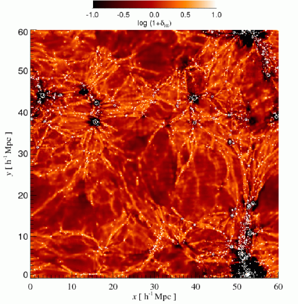
Figure 1: The spatial distribution of the neutral hydrogen overdensity in a slice of thickness 6 Mpc $h^{-1}$ (comoving) around the largest cluster in the simulation box (bottom–right part of the panel) extracted from the ESW simulation. White dots are drawn at the position of dark matter halos. Their size is proportional to the halo mass.

2.1 Mock galaxies

In the simulation we assume a one–to–one correspondence between gas-rich galaxies and their dark matter halo hosts. We extract halos using a friend–of–friend algorithm with a linking length which is 0.2 times the mean interparticle separation and consider only identified haloes in the mass range $[8\times 10^{10},\ 10^{13.5}\ {\rm M}_{\odot}\ h^{-1}]$. The lower limit is set (conservatively) by the numerical resolution while the upper limit avoids including large halos associated with groups and clusters, rather than single galaxies. However, we have checked that including the few halos larger than $10^{13.5}\ {\rm M}_{\odot}$ does not affect the results presented in this work. The geometric mean mass of the haloes is $\sim 2.46\times 10^{11}\ {\rm M}_{\odot}\ h^{-1}$, to be compared with a mean mass $10^{11}\ {\rm M}_{\odot}\ h^{-1}$ associated to dark matter halos hosting HIPASS galaxies (RW06, Mo et al. (2005)). The space density of these mock galaxies (0.0023 per cubic Mpc $h^{-1}$ comoving) is similar to that of HIPASS galaxies in the volume limited sample of Meyer et al. (2007) [M07] ($\sim 0.003$ per cubic Mpc $h^{-1}$). This sample contains all galaxies within 30 Mpc $h^{-1}$ and HI mass above $10^{9.05}\ {\rm M}_{\odot}\ h^{-2}$, corresponding to a halo mass of $\sim 10^{11}\ {\rm M}_{\odot}\ h^{-1}$, as inferred from the Mo et al. (2005) model, i.e. similar to our lower mass cut off. As we shall see in Section 4 the spatial two-point correlation function of these mock galaxies matches that of the HIPASS objects, hence fulfilling the main requirement of our analysis.

The mock galaxies extracted from the three simulations are hosted in the same dark matter haloes that, however, have a different baryon (gas+star) content. The baryon mass in the mock galaxies is affected by galactic winds and star formation processes. The mean baryonic mass measured in the NW, SW and ESW simulations is respectively $4.7\,,\ 2.1\ {\rm and}\ 1.9\times 10^{10}\,\ {\rm M}_{\odot}\ h^{-1}$, thus indicating that galactic winds are quite effective in blowing baryons out of dark halos. The star formation mechanism also plays a role: the mean stellar mass of $3.0\times 10^{10}\,\ {\rm M}_{\odot}\ h^{-1}$ in the NW simulation decreases to $0.6\ {\rm and}\ 0.5\times 10^{10}\,\ {\rm M}_{\odot}\ h^{-1}$ in the SW and ESW experiments that adopt the multiphase criterion.

To better investigate the dependence of the spatial correlation on the galaxy mass we have divided, for the NW case only, the mock galaxy sample by mass in two subsets. The characteristics of all mock galaxy samples considered in this paper are summarized in Table 2.

Finally, to compute the correlation properties of the mock galaxies we have generated a random galaxy sample by randomly positioning $5\times 10^{4}$ objects in the simulation volume.

Mock Galaxy Samples
Sample	Ngal	${\rm M}_{\rm Min}$	${\rm M}_{\rm Max}$	$\langle{\rm M}_{\rm DM}\rangle$	$\langle{\rm M}_{\rm bar}\rangle$	Wind
GNW	4980	8.0	3160	24.6	4.7	NW
HG	2480	19	3160	53.4	10.9	NW
LG	2500	8.0	19	11.4	2.0	NW
GSW	4980	8.6	3128	25.6	2.1	SW
GESW	4980	8.6	3100	25.4	1.9	ESW

Table 2: Mock Galaxy Samples. Column 1: Sample name. Column 2: Number of mock galaxies. Column 3. Minimum dark halo mass. Column 4. Maximum dark halo mass. Column 5. Geometric mean dark halo mass. Column 6. Geometric mean baryonic mass. Column 7. Wind Model. All masses are in $10^{10}\mbox{$M_{\odot}$}\ h^{-1}$ units.

2.2 Mock Ly$\alpha$  absorbers

The computational box was pierced with 999 straight lines running parallel to the three Cartesian axes. Three sets of 333 mock Ly$\alpha$  absorption spectra along each axis were simulated and analyzed, both in real and redshift–space, to measure the position of each Ly$\alpha$  line and the column density of the associated HI absorber. In this work we only consider weak Ly$\alpha$  absorbers with column densities in the range $12.41\leq\log(\mbox{$N_{\rm HI}$}/$cm^-2$)\leq 14.81$ to match the characteristics of the RW06 sample.

The total number of absorbers increases slightly in presence of winds, while their average column density decreases, as shown in Table  3. However, the differences are small, especially between the SW and ESW experiments. The density of Ly$\alpha$  absorbers along the line–of–sight in the NW simulation ($\sim 10^{-3}\ {\rm km}^{-1}{\rm s}$) is larger than in the RW06 sample ($\sim 4\times 10^{-4}\ {\rm km}^{-1}{\rm s}$).

To investigate the significance of this mismatch we have computed the number of Ly$\alpha$ absorbers in our mock spectra, per unit redshift and column density in each of the three simulations and compared it with that measured by Penton et al. (2004) in the Space Telescope Imaging Spectrograph (STIS) QSO spectra. The results are shown in fig. 2. The solid, red curve refers to the NW simulation. The short–dashed green and the dot-dashed blue curves represent the Ly$\alpha$  lines in the SW and ESW runs, respectively. The distribution of the absorbers is robust to the presence of galactic winds. When compared to the STIS data of Penton et al. (2004) (long–dashed black curve) we note that the number of absorbers predicted by the simulation is larger than the observed ones over most of the $N_{\rm HI}$  range sampled by RW06 (indicated by the two vertical dotted lines). The difference between models and data, however, is well within observational errors of $\sim 1$ dex for $\log(\mbox{$N_{\rm HI}$}/$cm^-2$)\leq 14.5$ (Penton et al. (2004)). Since we expect that similar observational errors for RW06 absorbers, we conclude that there is no significant difference in the number density of mock and RW06 Ly$\alpha$  lines.

To investigate the dependence of the clustering properties on the absorber column density we have set a column density threshold $N_{\rm HI}$ $=10^{13.24}$ cm^-2which divides the sample in two equally large subsets and sorted all mock absorbers in the NW simulation by column density.

The main characteristics of each mock absorber sample are listed in Table 3. Moreover, since these mock sample contains many more spectra than in the real case, we have also extracted several absorbers’ sub–samples of 27 lines–of–sights to mimic the RW06 sample and assess the sampling noise.

Finally, to compute the two–point spatial correlation functions, we have generated random absorber samples by randomly positioning 50 Ly$\alpha$  absorption lines along the same 999 lines–of–sight used for the mock Ly$\alpha$  absorption spectra. We verified that the estimation of the correlation function does not change significantly if, instead, we consider 999 randomly chosen lines–of–sight for the random absorber samples. We note that 50 lines per spectra represents a good compromise between accuracy and computing time since doubling the number of random absorbers does not modify our estimates of $\xi$.

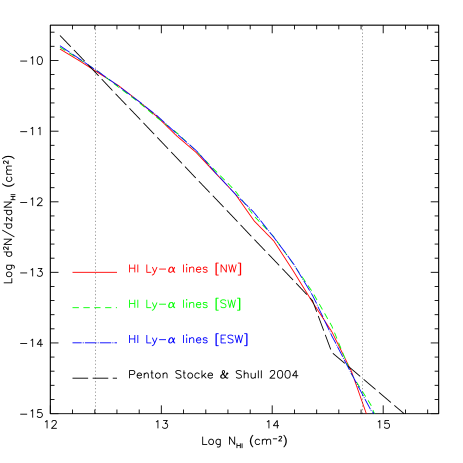
Figure 2: Number of Ly$\alpha$  absorbers per unit redshift and column density. Solid red line: NW simulation. Dashed green line: SW simulation. Dot–dashed blue line: ESW simulation. Dashed black: (Penton et al., 2004) best fit.

Mock Absorber Samples
Sample	NAbs	$N_{\rm HI}$Min	$N_{\rm HI}$Max	Wind
A NW	6239	12.41	14.81	NW
HA	1917	13.24	14.81	NW
LA	4322	12.41	13.24	NW
ASW	6444	12.41	14.81	SW
AESW	6445	12.41	14.81	ESW

Table 3: Absorber Samples. Column 1: Sample name. Column 2: Number of mock Ly$\alpha$  absorbers. Column 3. Minimum column density. Column 4. Maximum column density. Column 5. Wind model. All column densities are in $\log($cm^-2$)$ units.

3 Correlation Estimators

In this work we use the Davis & Peebles (1983) estimator to compute the galaxy–absorber cross–correlation function both in real and redshift–space, $\xi(r_{p},\pi)$ as:

$$\xi(r_{p},\pi)=\frac{AG(r_{p},\pi)}{RG(r_{p},\pi)}\frac{n_{RG}}{n_{AG}}-1,$$ (3)

where $AG(r_{p},\pi)$ is the number of mock absorber–galaxy pairs with projected separation, $r_{p}$ in the range $[r_{p}-\delta r_{p}/2,r_{p}+\delta r_{p}/2]$, and separation along the line–of–sight, $\pi$, in the range $[\pi-\delta\pi/2,\pi+\delta\pi/2]$. $RG(r_{p},\pi)$ is the number of pairs consisting of a random absorber and a mock galaxy. In both axes the binning $\delta\sigma$ and $\delta\pi$ is set at 0.39 $h^{-1}_{100}$ Mpc, i.e. 4 times wider than in RW06. The pair counts are divided by the total number of random–galaxy pairs $n_{RG}$, and galaxy–absorber pairs, $n_{AG}$. The separations $r_{p}$ and $\pi$ between two objects are computed from their recession velocities $\mbox{\bf v}_{i}$ and $\mbox{\bf v}_{j}$ according to (Fisher et al., 1994):

$$\pi=\frac{\mbox{\bf l}\cdot\mbox{\bf s}}{H_{0}|\mbox{\bf l}|},\ \ \ \ r_{p}=\frac{\mbox{\bf s}\cdot\mbox{\bf s}}{H_{0}^{2}}-\pi^{2}$$ (4)

where $\mbox{\bf l}\equiv(\mbox{\bf v}_{1}+\mbox{\bf v}_{2})/2$ and $\mbox{\bf s}\equiv\mbox{\bf v}_{1}-\mbox{\bf v}_{2}$. The estimator (3) is evaluated in the range of separations [0, 50] Mpc $h^{-1}$both along $r_{p}$ and $\pi$ directions. To estimate the galaxy–absorber correlation function in redshift–space we have used the distant observer approximation, i.e. we have counted the galaxy–absorber pairs in each of the three subsets of mock spectra parallel to one Cartesian axis and considered only the corresponding component of the peculiar velocity to compute the redshift. The rationale behind this choice is to detect and average out possible geometrical distortions arising, for example, when lines–of–sights are oriented along HI-rich gas filaments or when a large fraction of mock galaxies belong to some prominent, anisotropic cosmic structure.

The galaxy–galaxy and absorber–absorber auto–correlation functions are calculated in a similar way, i.e. by counting galaxy–galaxy and absorber–absorber rather than galaxy-absorbers pairs. The spherical average of $\xi(\sigma,\pi)$ gives the spatial correlation function $\xi(s)$ where $s=\sqrt{r_{p}^{2}+\pi^{2}}$. We also estimate the analogous quantity in real–space, $\xi(r)$, where $r$ represents the genuine pair separation that coincides wit their redshift difference in absence of peculiar velocities. In order to compare our result with those of RW06 we compute two more quantities. The first one is the projected correlation function, $\Xi(r_{p})$:

$$\Xi(r_{p})=2\int_{0}^{\pi_{max}}\xi(r_{p},\pi)d\pi,$$ (5)

where $\pi_{max}=50\ \mbox{Mpc $h^{-1}$}$.

The second one is the absorber auto–correlation along individual lines–of–sight,

$$\xi(\pi)=\frac{AA(\pi)}{AR(\pi)}\frac{n_{AR}}{n_{AA}}-1,$$ (6)

where $AA(\pi)$ is the number of mock absorber pairs with separation $\pi$ along the line–of–sight and $AR(\pi)$ is the number of random absorber pairs.

The uncertainties in the cross and auto–correlation functions of the mock samples are computed using the bootstrap resampling technique. For large, independent datasets bootstrap errors are equivalent to uncertainties calculated using the jackknife resampling, as in RW06. The uncertainty is computed in each $(r_{p},\pi)$ bin as

$$\sigma_{\xi_{i}}^{2}=\frac{\sum_{j=1}^{N}{\left(\bar{\xi_{i}}-\xi_{i}^{j}\right)}^{2}}{N-1},$$ (7)

where the subscript _i identifies the bin, _j refer the sample and $\bar{\xi_{i}}$ is the average correlation function computed over the $N$ bootstrapped samples. In this work $N=50$ which provide us with a robust error estimate (increasing $N$ to 350 modifies errors by $<2\%$).

This error estimate assumes that the covariance matrix of the data is diagonal, i.e. that the values of $\xi(\sigma,\pi)$ in different bins are not independent, which is known not to be the case. However, our simple way of estimating the uncertainties avoids the complication of dealing with a large covariance matrix, while providing an unbiased estimate of the real errors (Hawkins et al., 2003).

4 Real–Space Analysis

In this analysis we ignore peculiar velocities when we use Eq. 4 to estimate $r_{p}$ and $\pi$ from redshifts. In Fig. 3 we show the real–space auto–correlation function of the mock galaxies in the G_NW sample (black dots). Errorbars represent 1-$\sigma$ bootstrap uncertainties. The autocorrelation of mock galaxies is shown together with that of HIPASS galaxies, indicated by the dashed line which represents the power–law best fit to the $\xi(r)$ in the volume–limited sub-sample of galaxies extracted from the HIPASS catalog by M07. This power–law has a slope $\gamma_{gg}=1.5\pm 1$ and correlation length $r_{0,gg}=3.2\pm 1.4$ Mpc $h^{-1}$. The two functions agree, within the errors, below $10\ \mbox{Mpc $h^{-1}$}$, since the power–law fit to the correlation function of our mock galaxies in the range $[1,10]\ \mbox{Mpc $h^{-1}$}$ has $\gamma_{gg}=1.46\pm 0.03$ and $r_{0,gg}=3.06\pm 0.15$ Mpc $h^{-1}$. We have considered the M07 result since it is based on a sub-catalog that is volume limited, like our mock samples but it is worth noticing that the RW06 fit obtained using the full, flux limited HIPASS sample is fully consistent with the M07 result and, therefore, with our fit too.

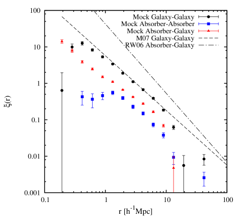
Figure 3: The real–space two–point correlation functions of the mock galaxy and absorber samples. Black dots: galaxy auto–correlation function in the G_NW-sample. Blue squares: absorber autocorrelation function in the A_NW–sample. Red triangles: galaxy–absorber autocorrelation function in the A_NW+G_NW sample. The size of the bars shows 1-$\sigma$ bootstrap resampling uncertainties. Black dashed curve: best fit to the galaxy–galaxy correlation function in the HIPASS volume–limited sample of M07. Black dot–dashed curve: RW06 best fit to the HIPASS galaxy- Ly$\alpha$  absorbers cross–correlation function.

The correlation signal of the mock galaxies suddenly drops at separations smaller than 0.4 Mpc $h^{-1}$. On the contrary, the galaxy correlation function of RW06 monotonically increases when reducing the pair separation. Including the few mock halos larger than $10^{13.5}\mbox{$M_{\odot}$}$ sample does not modify significantly this small-scale trend. This small–scale mismatch as an artifact deriving from the fact that, in the simulation, we do not resolve galaxy–size sub–structures within the large cluster–size halos that, if present, would significantly contribute to the correlation signal at sub–Mpc $h^{-1}$scales. Indeed, when we run the Friends–of–Friends algorithm to identify halos using a smaller linking length of 0.1 times the mean inter–particle spacing, the small scale flattening disappears and the power–law behavior is restored below 0.3 Mpc $h^{-1}$.

Mock absorbers are significantly less self–clustered than galaxies: their autocorrelation function (blue squares) is factor of $\sim 10$ below that of galaxies (see Dobrzycki et al. (2002)). We cannot compare this result with observational data directly, since the observed Ly$\alpha$  absorbers are too sparse. However, RW06 was able to compute their correlation along each line–of–sight and we compare this result with the theoretical predictions in the next Section.

The red triangles show the mock galaxy–absorber cross–correlation function of the A_NW+G_NW samples which is significantly weaker than the galaxy auto–correlation. This result is at variance with that of RW06 who find that the cross–correlation function of HIPASS galaxies and Ly$\alpha$  absorbers (dot–dashed curve in Figure 3) in the $[1,10]$ Mpc $h^{-1}$range is best fitted with a power–law slope $\gamma_{ag}=1.9\pm 0.3$ and correlation length $r_{0,ag}=7.2\pm 1.4$ Mpc $h^{-1}$, significantly larger than that of the galaxy auto–correlation function. When we fit the cross–correlation function of the mock data in the same range of separations we find $\gamma_{ag}=1.29\pm 0.03$ and correlation length $r_{0,ag}=1.44\pm 0.08$ Mpc $h^{-1}$.

RW06 pointed out that the cross–correlation signal increases with the column density of the absorber. We find the same trend in the simulation. We show in Fig. 4, the cross–correlation signal increases when we restrict our analysis to strong absorbers of the HA sample. On the contrary, massive mock galaxies do not seem to be significantly more or less correlated to Ly$\alpha$  absorbers than smaller galaxies. In fact, we find that the cross–correlation signal is almost independent of galaxy mass.

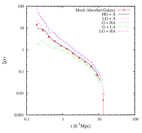
Figure 4: The absorber–galaxy cross–correlation function in various mock subsamples. Red triangles with errorbars: A_NW+G_NW sample. Black solid line: HG+A_NW. Dashed red: LG+A_NW. Dotted blue: G_NW+HA. Dot-dashed green: G_NW+LA. Long-dashed magenta: LG+HA.

Strong galactic winds can blow gas out of galaxy–size halos and therefore could suppress the cross–correlation signal on sub-Mpc scales. To quantify the effect we have computed the galaxy–absorber correlation functions in the SW and ESW simulations and compared them with that of the NW experiment. The results are shown in Fig. 5. The red triangles with errorbars represent the same cross–correlation function of the A_NW+G_NW sample shown in Fig. 4 and refer to the case of no winds. The effect of including the effect of strong winds is illustrated by the blue dashed and solid black curves that refer to the SW and ESW simulations, respectively. Even adopting extreme prescriptions for galactic winds, the effect on the galaxy–absorber correlation function is very small and, as expected, is significant only at separations $\lesssim 0.3\,\mbox{Mpc $h^{-1}$}$ where fewer galaxy–absorber pairs are found with respect to the NW case. This is not surprising, considering the free travel length $l_{w}$ adopted in the models. We find no significant differences between the SW and ESW experiments, which illustrates the robustness of the cross–correlation signal on scales larger than $l_{w}$ to the scheme adopted to simulate galactic winds.

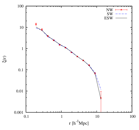
Figure 5: Effect of galactic winds on the cross-correlation function. Red triangles: A_NW+G_NW samples in the NW simulation. Dashed blue curve: SW simulation. Solid, black curve: ESW simulation. The size of the bars shows 1-$\sigma$ bootstrap resampling errors.

5 Redshift–Space Analysis

In Section 4 we have shown that hydrodynamical simulations do not reproduce the RW06 result. On the contrary, the galaxy-absorber correlation function is significantly weaker than the galaxy autocorrelation function. The previous analysis, however, has been performed in real–space ignoring peculiar velocities that may bias the correlation analysis. Moreover we have considered a number of spectra much larger than that of RW06. Therefore, we must account for the possibility is that the mismatch between hydrodynamical simulations and RW06 is not genuine but derives, instead, from redshift–space distortions and sparse HI sampling that, if not properly accounted for, may affect the cross-correlation analysis. In an attempt to account for both types of errors we repeat the correlation analysis using more realistic mock catalogs in which redshifts are used as distance indicators and only 27 lines-of-sight are taken to mimic the RW06 data set. To investigate the two effects separately, we first perform a redshift–space analysis of the whole A_NW+G_NW sample and then we consider sub-samples of 27 lines-of-sight.

In Figure 6 the autocorrelation function of the mock galaxies in the G_NW sample, $\xi_{gg}(r_{p},\pi)$, is plotted on the $(r_{p},\pi)$ plane. Contours are drawn at iso–correlation levels of 2,1,0.5,0.25. The distortions along the $\pi$ axis induced by small scale incoherent motions within virialized structures (the so called fingers–of–god) can be seen at separations $r_{p}\leq 2\,\mbox{Mpc $h^{-1}$}$ extending out to $\pi=6$ Mpc $h^{-1}$. A similar distortion pattern is seen in the correlation function of HIPASS galaxies (Fig. 2 of RW06). In that case a second, independent, distortion pattern along the $r_{p}$ axis, is detected at separations $r_{p}\gtrsim 4\,\mbox{Mpc $h^{-1}$}$. The compression of the isodensity contours along $\pi$ is the signature of large scale coherent motions that increase the apparent number of pairs with large separations. This second distortion pattern is not visible in Fig. 6, a fact that we ascribe to the lack of large scale power in our simulations. Indeed, our simulations do not account for power on scales larger than 60 Mpc $h^{-1}$which could significantly contribute to the amplitude of the bulk motions and thus to the compression of the iso–density contours.

Figure 6: The redshift–space auto–correlation function $\xi_{gg}(r_{p},\pi)$ of mock galaxies in the G_NW sample. The binning is 0.4 Mpc $h^{-1}$in both axis. Iso-correlation contours are drawn at correlation levels of 2,1,0.5,0.25. Bootstrap resampling shows typical pixel variations of the order $\xi(r_{p},\pi)\sim 0.08$

Figure 7 shows the redshift–space cross–correlation function $\xi_{ag}(r_{p},\pi)$ of mock absorbers and galaxies in the A_NW+G_NW sample. The signal is significantly weaker than the galaxy auto–correlation and the distortion pattern looks very different as no significant elongation is seen along the $\pi$ axis. Instead, at large separations, the iso–correlation contours are compressed along $\pi$, as expected in the presence of coherent motions. The differences between $\xi_{ag}(r_{p},\pi)$ and $\xi_{gg}(r_{p},\pi)$ reveal that mock Ly$\alpha$  absorbers and galaxies have different dynamical properties. Galaxies’ relative velocities are dominated by the incoherent motions, typical of virialized structures. Instead, the relative motion of mock Ly$\alpha$  absorbers and galaxies is more coherent, suggesting that mock absorbers are preferentially located in the outskirts of high density regions into which they are probably falling.

Finally, we note that the peak of the cross-correlation function is spatially offset from the center. This feature and the general distortion pattern of the simulated cross-correlation function are qualitatively similar to that of the cross-correlation function between the CHFT galaxies and the $HST$ Quasar Absorption Line Key Project Data Release Ly$\alpha$   with $13\leq\log(\mbox{$N_{\rm HI}$}/$cm^-2$)<15$ measured by W07. On the contrary, the RW06 cross-correlation function is dominated by a very large finger–of–god distortion. A similar, but less prominent, distortion pattern has been seen by Davé et al. (1999) and W07 in their numerical experiments. RW06 interpreted this distortion as the draining of the gas from low-density regions into collapsed structure. Although the dynamical interpretation in this case is not as simple as in the galaxy-galaxy case, we note that the draining mechanism advocated by RW06 would probably lead to coherent, rather than incoherent motions, which would produce a very different distortion pattern. W07 suggested that the finger–of–god distortion could be a geometrical effect deriving from observing Ly$\alpha$  absorbers along lines–of–sights that run along some radially-elongated structure. To check this hypothesis we exploited the distant observer approximations and computed the cross-correlation function by considering redshift distortions along one Cartesian axis at a time. If distortions were purely geometric, i.e. induced by a few prominent, anisotropic structures, we would expect to see different distortion patterns in the cross-correlation functions computed along orthogonal axes. If, on the other hand, they were caused by random motions within large, spherically symmetric, virialized structures like galaxy clusters, we would expect to see fingers-of-god type distortions along all axes. Instead, the correlation functions measured by three, orthogonally–positioned distant observers turned out to be very similar and consistent with the one shown in Fig. 7. We conclude that neither pure geometrical effects nor incoherent motions can alone explain the distortion pattern in the $\xi_{ag}(r_{p},\pi)$ of our mock A_NW+G_NW samples.

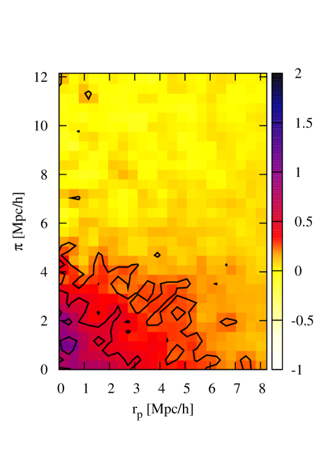
Figure 7: The redshift–space cross–correlation function $\xi_{ag}(r_{p},\pi)$ of mock absorbers and galaxies in the A_NW+G_NW sample. The binning is 0.4 Mpc $h^{-1}$in both axis. Iso-correlation contours are drawn at correlation levels of 1,0.5,0.25. Bootstrap resampling shows typical pixel variations of the order $\xi(r_{p},\pi)\sim 0.2$

Small redshift distortions could be amplified by sampling Ly$\alpha$  absorbers along a limited number of lines–of–sights, as in the RW06 case. To quantify the effect of shot noise errors coupled to dynamical and geometrically–induced distortions, we have constructed 30 independent realistic mock Ly$\alpha$  sub-samples of 27 independent lines–of–sights and computed their cross–correlation with all mock galaxies of the G_NW sample. In Fig. 8 we show $\xi_{ag}(r_{p},\pi)$ computed in four such realistic mock samples. The cross-correlation functions shown in the two upper panels are characterized by prominent finger–of–god distortions which, in the upper–right plot, are similar in amplitude to that measured by RW06. This kind of distortion is found in $\sim 20\%$ of the mock subsamples considered. The fact that we observe fingers–of–god distortions along different Cartesian axes suggest that they cannot be attributed to the fact that the sample is dominated by a single, prominent, anisotropic structure. Rather, they seem to originate from genuine, finger–of–god like, dynamical distortions which become apparent when a significant fraction of the 27 spectra samples some virialized regions. The relevance of sparse sampling variance in the cross-correlation analysis is even more evident in the two bottom panels of Fig. 8. They show the cross–correlation function computed along the same ($Z-$) axis, as in the top–right panel, but use two independent sets of lines–of–sight. Not only the finger–of–god distortion disappears but the cross–correlation signal is either very weak (bottom left) or significantly offset from the center (bottom-right).

A more quantitative assessment of sparse sampling errors is given in Fig. 9 in which we show the projected absorber-galaxy cross correlation function $\Xi_{ag}(r_{p})/r_{p}$ of the A_NW+G_NW sample (filled black dots). Small errorbars drawn with solid lines represent 1-$\sigma$ bootstrap resampling errors computed using all 999 mock absorbers in the A catalog. Large errorbars plotted with dashed lines represent the scatter around the mean of the projected cross–correlation function computed using the 30 realistic mock absorbers’ samples consisting of 27 lines–of–sight. The sampling noise clearly dominates the error budget and the total error significantly exceeds that of RW06. Filled red squares show the projected galaxy-galaxy correlation function with the 1-$\sigma$ bootstrap errors. In order to assess the goodness of our error estimate we have compared the scatter among the 30 catalogs with the bootstrap errors computed from N=50 samples. The two errors agree well in the range (1,10) Mpc/h, in which boostrap errors are $\sim 15\ \%$ smaller than those shown in Fig.  9. On smaller scales the bootstrap resampling technique overestimates the errors by factor of $\sim 2$. The autocorrelation signal is higher than the cross–correlation one, consistently with the real–space analysis. However, the difference is of the order of the errors, i.e. the mismatch is about 1-$\sigma$ at separations $r_{p}>1\,\mbox{Mpc $h^{-1}$}$, in the range in which RW06 find that the cross-correlation signal is larger than the autocorrelation one. Filled triangles show the projected autocorrelation function of all absorbers in the A_NW sample. As anticipated by the real–space analysis, absorbers correlate with themselves very weakly. When one accounts for sparse sampling their autocorrelation signal is consistent with zero.

RW06 were able to detect the auto-correlation signal of the absorbers by measuring their auto-correlation function $\xi(\pi)$ of eq. 6 along individual lines–of–sight. We have repeated that analysis using all absorbers in the A sample. The resulting auto-correlation function replicates the RW06 result to within 1-$\sigma$.

Finally, to test the robustness of our results we have computed the cross–correlation function, $\xi_{ag}(r_{p},\pi)$ using the HG, LG, and LA sub–samples as well as the mock catalogs extracted from the SW and ESW runs. There are no cases in which wer are able to obtain a galaxy–galaxy autocorrelation signal weaker than the cross–correlation one and to reproduce the large finger–of–god distortion feature observed by RW06.

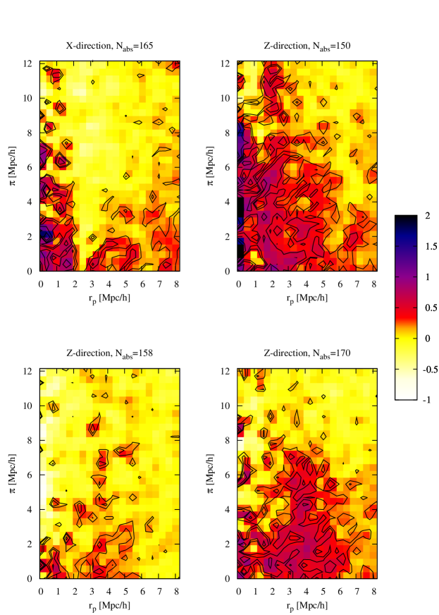
Figure 8: The redshift–space absorber–galaxy cross–correlation function $\xi_{ag}(r_{p},\pi)$ for four independent subset of absorbers along 27 lines–of–sight. On top each panel is indicated the direction along which absorptions spectra were drawn and the total number of mock absorbers in each sample N_abs. All cross–correlation functions are computed using the same 4980 mock galaxies in the G sample.

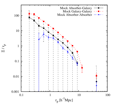
Figure 9: Filled dots and solid line: projected absorber-galaxy cross correlation function $\Xi_{ag}(r_{p})/r_{p}$. Small errorbars are 1-$\sigma$ bootstrap resampling errors. Large errorbars account for sparse sampling variance. Filled squares and dashed line: galaxy-galaxy projected autocorrelation function $\Xi_{ag}(r_{p})/r_{p}$. Filled triangles and dot-dashed line: absorber-absorber projected autocorrelation function $\Xi_{aa}(r_{p})/r_{p}$

6 Conclusions

In this work we have studied the relative spatial distribution of galaxies and weak Ly$\alpha$  absorbers with $12.41\leq\log(\mbox{$N_{\rm HI}$}/$cm^-2$)\leq 14.81$ in hydrodynamical simulations and compared our results with the analyses of real datasets performed by W07 and, mainly, with RW06. Our main conclusions are:

• The galaxy-absorber two-point cross-correlation function in the hydrodynamical simulation is weaker than the galaxy auto-correlation function. This result is at variance with that of RW06 but in qualitative agreement with the analysis of W07.

• No flattening at small separation is observed in the cross correlation function of all mock absorbers, unlike in RW06. A small-scale flattening is observed, however, when the cross correlation analysis is restricted to low density absorbers.

• The cross correlation signal increases with the column density of the absorbers, in agreement with RW06. We find no significant dependence on galaxy mass.

• Galactic winds have a small effect on the absorber and galaxies correlation properties in these models. Using the most extreme prescription to simulate these winds suppresses the cross-correlation signal only at separations $\lesssim 0.3\ \mbox{Mpc $h^{-1}$}$.

• Absorbers correlate with themselves more weakly than with galaxies. Their auto–correlation signal is very weak and consistent with that measured by RW06.

• Redshift–space distortions alone cannot explain two aspects of the differences with the RW06 results. The cross–correlation signal is weaker than the galaxy auto–correlation signal. The two-point cross–correlation function, $\xi_{ag}(r_{p},\pi)$ does not show a prominent finger–of–god type of distortion. The latter looks very prominent in the RW06 cross–correlation function but is not seen in the W07 one.

• The origin of the finger–of–god distortion cannot be purely geometric, i.e induced by the presence of a prominent, anisotropic structure in the sample. In this case distant observers taking spectra along orthogonal directions would detect different distortion patterns. We do not see such effect.

• Fingers–of–god distortions may appear when sampling the intergalactic gas using a limited number of UV spectra, as in the RW06 sample. In this case, they represent genuine dynamical distortions that become apparent when a few spectra, that however represent a significant fraction of the total, pierce some virialized regions.

• The sampling noise is large. Once accounted for, the difference between the simulated galaxy–galaxy and galaxy–absorber correlation functions is significant at the $\sim 1$-$\sigma$ level only.

7 Discussion and perspectives

Modeling the gas distribution in the low redshift universe is a difficult task. Numerical experiments use a number of simplifying hypothesis and approximations that potentially affect our results. The main uncertainties are related to the ill-known mechanisms of stellar feedback and galactic winds for which we have adopted simplistic phenomenological prescriptions. It is therefore very reassuring that our results are robust to the star formation criterion and galactic wind prescriptions adopted. However, since robustness does not exclude systematic errors one needs to be aware that the various approximations adopted in our numerical model to predict the HI distribution at $z=0$ may bias our results.

Our model does not include halos larger that $10^{13.5}\ \mbox{$M_{\odot}$}$ and ignores substructures within virialized halos. While we have checked that including large halos does not change our results, ignoring galaxy-size halos within groups or clusters may affect the outcome of the correlation analysis. Galaxies in strongly clustered environments significantly contribute to both the auto- and the cross-correlation function at small separations. Ignoring their presence would artificially decrease the correlation signal, producing a flattening in the correlation functions at small separations. We do see a flattening but only in the galaxy-autocorrelation function and on scales smaller than 0.4 Mpc $h^{-1}$. The cross–correlation function, instead, increases at small separations unlike the one of RW06 that flattens and we do not reproduce the flattening at separations smaller than 1 Mpc $h^{-1}$. A flattening of the galaxy-absorber cross-correlation function at small scales was also seen in the numerical simulations of Davé et al. (1999) that, however, have a limited resolution compared to ours. The fact that we find no flattening in the cross-correlation function has two implications. First, ignoring sub-clustering within large halos has little impact on our results. Second, it seems that there is no characteristic scale for the cosmic structures in which Ly$\alpha$  absorbers are embedded.

The RW06 analysis convincingly rules out minihaloes for the confinement of weak Ly$\alpha$  absorbers. Based on the measured cross-correlation strength, RW06 suggest that they are embedded in much larger halos with the typical mass of a galaxy-group. This would imply a self–clustering of the absorbers comparable or even larger than that of galaxies. The fact that, on the contrary, the measured absorber self–clustering along the line–of–sight is weak is not regarded by RW06 as a conclusive evidence since redshift distortions may artificially dilute the correlation signal. Our numerical experiments provide a direct estimate for the self–clustering of the absorbers which is free of redshift–distortions. The real–space analysis we have performed indicates that the auto-correlation function of the mock absorbers is significantly weaker than that of mock galaxies and that, in redshift–space, their self–clustering is consistent with the RW06 estimates. The outcome of our numerical model suggest therefore that in a $\Lambda$CDM universe weak Ly$\alpha$  absorbers are not embedded in group-size halos. In fact, the association of weak Ly$\alpha$  absorbers with virialized halos is probably too naive. The absence of a strong finger–of–god distortions in the simulated $\xi_{ag}(r_{p},\pi)$ suggest that the neutral hydrogen responsible for weak Ly$\alpha$  absorption lines is not part of virialized structures. Rather, it is probably located in their outskirts, in–falling towards their central regions. Interestingly, we see a flattening in the absorber auto–correlation function at separations $\lesssim 1\,\mbox{Mpc $h^{-1}$}$ a feature which is also typical of the the warm–hot intergalactic gas according to both numerical (Davé et al., 2001) and semi-analytic (Valageas et al., 2002) predictions.

Finally, we turn to what we regard as the main result of this work. RW06 find that the galaxy-absorber cross-correlation signal is significantly larger than the galaxy-galaxy correlation. Our numerical analysis is not able to reproduce the observation as we find that the opposite is true. However, when shot noise errors are accounted for, the discrepancy between the auto- and cross-correlation signals is of the order of 1-$\sigma$ only. Can we reconcile the two results ? Our numerical experiments were performed on a rather small box of $60\ \mbox{Mpc $h^{-1}$}$ which cannot be regarded as a fair sample of the universe. In other words our cosmic variance is not negligible and should be accounted for in our error budget. This would require running numerical simulations in a larger box while keeping the same resolution or running several identical simulations of different random realizations of the universe. In either case the likely outcome would be that of increasing the size of the errorbars in fig. 9 and the conclusion would be that, probing the HI distribution with 27 lines–of–sight is not sufficient, in a $\Lambda$CDM, universe to demonstrate a difference between the self and cross clustering of galaxy and Ly$\alpha$  absorbers at the level measured by RW06.

The fact that the errorbars in the projected cross-correlation function of RW06 are smaller than ours seem to indicate that their error estimates are biased low. In section 5 we have shown that the bootstrap technique underestimates errors by $\sim 15$ %, on average, at separations $\geq 1\mbox{Mpc $h^{-1}$}$ when the sampling is as sparse as in the RW06 case. This bias reflects the fact that absorbers are not guaranteed to be independent. It is plausible that this effect is even more severe in the RW06 sample since nearly 30% of the absorption spectra considered were drawn in the vicinity of the Virgo cluster region. We would also expect that these spectra could artificially amplify the cross–correlation signal since the Virgo cluster is an HI-rich region. However, surprisingly enough, the excess cross-correlation signal is still present when galaxies and absorbers from this region are excluded from the analysis (Ryan-Weber, private communication).

The only way out at this apparent paradox is that the relative distribution of galaxies and Ly$\alpha$  absorbers in the RW06 sample is different from that of the typical cosmic environment, since the cross-correlation signal and its variance are significantly different from their average values. This despite the fact that in our cosmic neighborhood the most prominent structures are anisotropically located along the Super-Galactic plane, rather than being homogeneously distributed. We see two possible ways to check the validity of this hypothesis. One is to resort to the so called constrained hydrodynamical experiments designed to match the actual gas distribution in our local universe (Kravtsov, Klypin & Hoffman, 2002; Klypin, Hoffman, Kravtzov, & Gottlober, 2003; Yoshikawa et al., 2005; Viel et al., 2005). Currently available simulations, however, are of little use as their constraints are either too weak, as they refer to scales larger than 5 Mpc $h^{-1}$(Gaussian), or too local, as they are effective out to distances of $\sim 15$ Mpc $h^{-1}$, i.e. within our local Supercluster. The second possibility, which looks more promising, is to improve the sampling of the HI distribution either through Ly$\alpha$  absorption lines in the UV absorption spectra or through the X-ray lines of highly ionized metals, like OVII. The latter is expected to trace the Warm Hot Intergalactic Medium (WHIM) in density-temperature environment similar to that in which the weak Ly$\alpha$  absorbers can be found. With this respect, proposed X-ray satellites like EDGE (Piro et al., 2005) are particularly interesting, as they could observe the WHIM in emission, which would allow one to trace the three dimensional gas distribution rather than probing it in 1D along a few lines–of–sight.

It is worth stressing that the present tension between model and data could be a signature of the fact that hydrodynamical simulations are still missing physical inputs able to reproduce the observations. However, if the mismatch between theory and observations is confirmed, which probably requires both better observational data and better control over systematics in the numerical models, the RW06 results could constitute an interesting challenge to the $\Lambda$CDM paradigm, similar, and perhaps related to the absence of dwarf galaxies in voids (Peebles, 2007).

References

- Adelberger et al. (2005) Adelberger K. L., Shapley A. E., Steidel C. C., Pettini M., Erb D. K., Reddy N. A., 2005, ApJ, 629, 636
- Bolton et al. (2007) Bolton J. S., Haehnelt M. G, 2007, MNRAS, 374, 493
- Bouché et al. (2007) Bouché, N. and Murphy, M. T. and Péroux, C. and Davies, R. and Eisenhauer, F. and Förster Schreiber, N. M. and Tacconi, L., 2007, ApJ, 669, L5
- Bowen et al. (2002) Bowen D. V., Pettini M., Blades J. C., 2002, ApJ, 580, 169
- Côté et al. (2005) Côté S., Wyse R. F. G., Carignan C., Freeman K. C., Broadhurst T., 2005, ApJ, 618, 178
- Chen et al. (2005) Chen H.-W., Prochaska J. X., Weiner B. J., Mulchaey J. S., Williger G. M., 2005, ApJ, 629, L25
- Churchill et al. (2007) Churchill, C. W. and Kacprzak, G. G. and Steidel, C. C. and Evans, J. L., 2007, ApJ, 661 714
- Davé et al. (1999) Davé R., Hernquist L., Katz N., Weinberg D. H., 1999, ApJ, 511, 521
- Davé et al. (2001) Davé R., Cen R., Ostriker J. P., Bryan G. L., Hernquist L., Katz N., Weinberg D. H., Norman M. L., O’Shea B., 2001, ApJ, 552, 473
- Davé et al. (2003) Davé R., Katz N., Weinberg D. H., 2003, in ASSL Vol. 281: The IGM/Galaxy Connection. The Distribution of Baryons at z=0, ASSL Conference Proceedings Vol. 281. Edited by Jessica L. Rosenberg and Mary E. Putman. Kluwer Academic Publishers, Dordrecht p. 271
- Davis & Peebles (1983) Davis M., Peebles P. J. E., 1983, ApJ, 267, 465
- Dobrzycki et al. (2002) Dobrzycki A., Bechtold J., Scott J., Morita M., 2002, ApJ, 571, 654
- Fisher et al. (1994) Fisher K. B., Davis M., Strauss M. A., Yahil A., Huchra J. P., 1994, MNRAS, 267, 927
- Grogin & Geller (1998) Grogin N. A., Geller M. J., 1998, ApJ, 505, 506
- Haardt & Madau (1996) Haardt F., Madau P., 1996, ApJ, 461, 20
- Hawkins et al. (2003) Hawkins E., et al., 2003, MNRAS, 346, 78
- Katz, Weinberg & Hernquist (1996) Katz N., Weinberg D. H., Hernquist L., 1996, ApJS, 105, 19
- Kravtsov, Klypin & Hoffman (2002) Kravtsov A. V., Klypin A., Hoffman Y., 2002, ApJ, 571, 563
- Klypin, Hoffman, Kravtzov, & Gottlober (2003) Klypin A., Hoffman Y., Kravtzov A. V., Gottlober S., 2003, ApJ, 596, 19
- Lanzetta et al. (1996) Lanzetta K. M., Webb J. K., Barcons X., 1996, ApJ, 456, L17
- Le Brun et al. (1996) Le Brun V., Bergeron J., Boisse P., 1996, A&A, 306, 691
- McLin et al. (2002) McLin K. M., Stocke J. T., Weymann R. J., Penton S. V., Shull J. M., 2002, ApJ, 574, L115
- Meiksin (2007) Meiksin A. A., 2007, ArXiv e-prints: 0711.3358
- Meyer (2003) Meyer M. J., 2003, Ph.D. Thesis, U. Melbourne
- Meyer et al. (2007) Meyer M. J., et al. 2007, ApJ, 654, 702
- Mo et al. (2005) Mo H. J., Yang X., van den Bosch F. C., Katz N., 2005, MNRAS, 363, 1155
- Morris & Jannuzi (2006) Morris S. L., Jannuzi B. T., 2006, MNRAS, 367, 1261
- Nagamine et. al. (2007) Nagamine, K. et al. 2007, ApJ, 660, 945
- Nestor et al. (2007) Nestor D. B., Turnshek D. A., Rao S.M., Quider A.M., 2007, ApJ, 658, 185
- Oppenheimer & Davé (2006) Oppenheimer, B. D. and Davé, R., 2006, MNRAS, 373, 1265
- Peebles (2007) Peebles P.J.E., 2007, arXiv:0712.2757
- Penton et al. (2002) Penton S. V., Stocke J. T., Shull J. M., 2002, ApJ, 565, 720
- Penton et al. (2004) Penton S. V., Stocke J. T., Shull J. M., 2004, ApJS, 152, 29
- Piro et al. (2005) Piro L., et al. 2007, arXiv:0707.4103
- Putman et al. (2006) Putman M. E., Rosenberg J. L., Stocke J. T., McEntaffer R., 2006, 131, 771
- Rosenberg et al. (2003) Rosenberg J. L., Ganguly R., Giroux M. L., Stocke J. T., 2003, ApJ, 591, 677
- Ryan-Weber (2006) Ryan-Weber E. V., 2006, MNRAS, 367, 1251
- Schaye et al. (2007) Schaye, J. and Carswell, R. F. and Kim, T.-S., 2007, MNRAS, 379, 1169
- Springel & Hernquist (2002) Springel V., Hernquist L., 2002, MNRAS, 333, 649
- Springel & Hernquist (2003) Springel V., Hernquist L., 2003, MNRAS, 339, 289
- Springel (2005) Springel V., 2005, MNRAS, 364, 1105
- Tripp et al. (2002) Tripp T. M., Jenkins E. B., Williger G. M., Heap S. R., Bowers C. W., Danks A. C., Davé R., Green R. F., Gull T. R., Joseph C. L., Kaiser M. E., Lindler D., Weymann R. J., Woodgate B. E., 2002, ApJ, 575, 697
- Valageas et al. (2002) Valageas P., Schaeffer R., Silk J., 2002, A&A, 388, 741
- Viel et al. (2004) Viel M., Haehnelt M. G., Springel V., 2004, MNRAS, 360, 1110
- Viel et al. (2005) Viel M., Branchini E., Cen R., Ostriker J.P., Matarrese S., Mazzotta P., Tully B., 2005, MNRAS, 354, 684
- Weymann et al. (1998) Weymann, R. J. and Jannuzi, B. T. and Lu, L. and Bahcall, J. N. and Bergeron, J. and Boksenberg, A. and Hartig, G. F. and Kirhakos, S. and Sargent, W. L. W. and Savage, B. D. and Schneider, D. P. and Turnshek, D. A. and Wolfe, A. M., 1998, ApJ, 506, 1
- (47) Wilman R. J., Morris S. L., Jannuzi B. T., Davé R., Shone A. L, 2007, MNRAS, 375, 735
- Wong, O. I. et al. (2006) Wong, O. I. et al. 2006, MNRAS, 371, 1855
- Yoshikawa et al. (2005) Yoshikawa K., et al. 2005, PASJ, 56, 939