Delocalization induced by nonlinearity in systems with disorder

Abstract

We study numerically the effects of nonlinearity on the Anderson localization in lattices with disorder in one and two dimensions. The obtained results show that at moderate strength of nonlinearity a spreading over the lattice in time takes place with an algebraic growth of number of populated sites $\Delta n\propto t^{\nu}$. This spreading continues up to a maximal dimensionless time scale $t=10^{9}$ reached in the numerical simulations. The numerical values of $\nu$ are found to be approximately $0.15-0.2$ and $0.25$ for the dimension $d=1$ and 2 respectively being in a satisfactory agreement with the theoretical value $d/(3d+2)$. During the computational times $t\leq 10^{9}$ the localization is preserved below a certain critical value of nonlinearity. We also discuss the properties of the fidelity decay induced by a perturbation of nonlinear field.

I Introduction

The phenomenon of the Anderson localization anderson1958 in systems with disorder has been extensively studied for electron transport and linear waves (see e.g. montambaux ). A remarkable experimental progress with the Bose-Einstein condensates (BEC) in optical lattices (see e.g. reviews pitaevskii ; oberthaler ; inguscio2008 ) stimulated the interest to investigations of the effects of nonlinearity on localization. At present the signatures of localization of BEC in one-dimensional (1D) optical disordered lattices have been detected by different experimental groups inguscio2005 ; aspect2005 ; inguscio12005 ; ertmer2005 ; aspect2006 . The effects of nonlinearity appear also for experiments with BEC in kicked optical lattices phillips2006 ; summy2006 ; steinberg where the quantum chaos in the Chirikov standard map (kicked rotator) chirikov is investigated. A similar type of problem also comes out for propagation of nonlinear waves in disordered photonic lattices which are now actively studied experimentally segev2007 ; silberberg2008 . In addition to that the problem of lasing in random media cao is also linked to the interplay of localization and nonlinearity that makes it related to the important field of nonlinear wave propagation in disordered media kivshar . In this work we concentrate our studies on the time dependent wave packet spreading in presence of disorder and nonlinearity leaving aside the problem of directed flow and scattering in nonlinear media (see e.g. Refs. in kivshar and more recent pavloff1 ).

The theoretical treatment of the interplay between localization and nonlinearity uses numerical simulations (see e.g. dls1991 ; dls1993 ; pavloff ; aspect2007 ; flach2008 ; dls2008 ; lebowitz ) and various analytical tools (see e.g. skipetrov2000 ; shapiro2007 ; wellens ; shapiro2008 ). However, even rather powerful analytical tools skipetrov2000 ; shapiro2007 ; wellens ; shapiro2008 do not allow to obtain the full solution of this rather complex problem. The existing rigorous mathematical results show that for a sufficiently small nonlinearity there exists a Kolmogorov-Arnold-Moser integrable localized regime for almost all initial conditions frolich but these results are applicable only to unrealistically small strength of nonlinearity. Due to that the numerical simulations become especially important for investigation of this problem. For numerical studies it is especially convenient to use a discrete lattice that allows to push numerical simulations to extremely large times. In addition to that the time evolution on a lattice is closely linked to the problem of energy propagation in complex molecules, e.g. proteins, where nonlinear couplings give transitions between localized linear modes james2005 ; flach2008 ; lebowitz . One of the examples of such a nonlinear oscillator chain is the Frenkel-Kontorova model in the pinned phase where the linear sound modes are localized in space zhirov .

Recently, the interplay of the Anderson localization and nonlinearity has been investigated by a number of mathematical methods where a certain number of interesting mathematical results has been obtained soffer ; wang1 ; wang2 . However, these methods still should be developed further to understand the asymptotic properties of spreading in the lattice at moderate strength of nonlinearity.

In this paper we further develop the old dls1991 ; dls1993 and recent studies dls2008 of the discrete Anderson nonlinear Schrödinger equation (DANSE) and present large scale numerical simulations of this model in one and two dimensions d (1D, 2D). In addition we perform numerical simulations for the kicked nonlinear rotator model (KNR) introduced in dls1993 . Our numerical results obtained on dimensionless time scales up to $t=10^{9}$ show that at moderate nonlinearity, above a certain threshold, the wave packet spreads unlimitedly over the lattice in such a way that the squared displacement of the packet on the lattice grows according to the algebraic law $R^{2}\propto t^{\alpha}$ with the exponent $\alpha\approx 0.3-0.4$ for $d=1$ and $\alpha\approx 0.25$ for $d=2$. This dependence is in a satisfactory agreement with the 1D estimates dls1993 which give $\alpha=2/5$ and the analytical estimates of this paper which give $\alpha=1/4$ for 2D. We also study the fidelity decay which shows interesting properties for the nonlinear evolution described by our model.

The paper is composed as follows: in Section II we give the model description and present simple estimates; the results for 1D and 2D are presented in Sections III and IV respectively, the properties of nonlinear fidelity decay are discussed in Section IV; the conclusions are given in Section V.

II Model description and analytical estimates

Our system is described by the DANSE model:

$$i\hbar{{\partial{\psi}_{\bm{n}}}\over{\partial{t}}}=E_{\bm{n}}{\psi}_{\bm{n}}+{\beta}{\mid{\psi_{\bm{n}}}\mid}^{2}\psi_{\bm{n}}+V({\psi_{\bm{n+1}}}+{\psi_{\bm{n-1}})}\;,$$ (1)

where $\beta$ characterizes nonlinearity, $V$ is a hopping matrix element on nearby sites, on-site energies are randomly and homogeneous distributed in the range $-W/2<E_{n}<W/2$, and the total probability is normalized to unity $\sum_{\bm{n}}{\mid{\psi_{\bm{n}}}\mid}^{2}=1$. Here, $\bm{n}$ is the lattice index, in 1D it is an integer, in 2D it is an integer vector of lattice indexes $\bm{n}=(n_{x},n_{y})$. For $\beta=0$ and weak disorder all eigenstates are exponentially localized with the localization length $l\approx 96(V/W)^{2}$ (1D) at the center of the energy band and $\ln l\sim(V/W)^{2}$ in 2D kramer1993 . Hereafter we set for convenience $\hbar=V=1$, thus the energy coincides with the frequency. We emphasize here that the DANSE (1) exactly describes recent experiments with one-dimensional disordered waveguide lattices (cf. Eq. (1) in silberberg2008 ), and it also serves as a paradigmatic model for a wide class of physical problems where interplay of nonlinearity and disorder is important. The DANSE can be considered as the Gross-Pitaevskii equation (GPE) pitaevskii taken on a discretized lattice. In 1D this model was studied recently in flach2008 ; dls2008 .

To understand the evolution properties of system (1) it is convenient to expand $\psi_{\bm{n}}$ in the basis of localized eigenmodes at $\beta=0$ dls1993 : $A_{\bm{n}}=\sum_{\bm{m}}Q_{{\bm{n}},{\bm{m}}}C_{\bm{m}}$ where $A$ and $C$ are amplitudes in the basis of sites and eigenmodes respectively. Due to the localization of linear eigenmodes with length $l$ we have for the transformation matrix $Q_{{\bm{n}}{\bm{m}}}\sim l^{-d/2}\exp(-|\bm{n}-\bm{m}|/l-i\chi_{{\bm{n}},{\bm{m}}})$, where $\chi$ are some random phases. From (1) it follows that the amplitudes $C$ in the linear eigenbasis are described by the equation

$$i{{\partial C_{\bm{m}}}\over{\partial{t}}}=\epsilon_{\bm{m}}C_{\bm{m}}+\beta\sum_{{\bm{m_{1}}}{\bm{m_{2}}}{\bm{m_{3}}}}V_{{\bm{m}}{\bm{m_{1}}}{\bm{m_{2}}}{\bm{m_{3}}}}C_{\bm{m_{1}}}C^{*}_{\bm{m_{2}}}C_{\bm{m_{3}}}$$ (2)

where $\epsilon_{\bm{m}}$ are the eigenmode energies. The transitions between linear eigenmodes appear only due to the nonlinear $\beta$-term and the transition matrix elements are $V_{{\bm{m}}{\bm{m_{1}}}{\bm{m_{2}}}{\bm{m_{3}}}}=\sum_{\bm{n}}Q^{-1}_{{\bm{n}}{\bm{m}}}Q_{{\bm{n}}{\bm{m_{1}}}}Q^{*}_{{\bm{n}}{\bm{m_{2}}}}Q_{{\bm{n}}{\bm{m_{3}}}}\sim 1/l^{3d/2}$ dls1993 . There are about $l^{3d}$ random terms in the sum in (2) with $V\sim l^{-3d/2}$ so that we have $idC/dt\sim\beta C^{3}$. We assume that the probability is distributed over $\Delta n>l^{d}$ states of the lattice basis. Then from the normalization condition we have $C_{\bm{m}}\sim 1/(\Delta n)^{1/2}$ and the transition rate to new non-populated states in the basis $\bm{m}$ is $\Gamma\sim\beta^{2}|C|^{6}\sim\beta^{2}/(\Delta n)^{3}$. Due to localization these transitions take place on a size $l$ and hence the diffusion rate in the distance $\Delta R\sim(\Delta n)^{1/d}$ of $d-$ dimensional $\bm{m}-$ space is $d(\Delta R)^{2}/dt\sim l^{2}\Gamma\sim\beta^{2}l^{2}/(\Delta n)^{3}\sim\beta^{2}l^{2}/(\Delta R)^{3d}$. At large time scales $\Delta R\sim R$ and we obtain

$$\Delta n\sim R^{d}\sim(\beta l)^{2d/(3d+2)}t^{d/(3d+2)}\;.$$ (3)

Thus as in dls1993 for $d=1$ we have $R^{2}\propto t^{2/5}$ and for $d=2$ this gives $R^{2}\propto t^{1/4}$, while for large $d$ the scaling is independent of $d$: $\Delta n\propto t^{1/3}$.

The relation (3) assumes that the dynamics of nonlinear chain (1) is chaotic. On a first glance it seems that it cannot be the case since as soon as $\Delta n$ grows with time the nonlinear frequency shift $\delta\omega\sim\beta|\psi_{n}|^{2}\sim\beta/\Delta n$ decreases. However, the physical importance relays not on the shift value itself but on its ratio to a frequency spacing between frequencies of excited modes which is $\Delta\omega\sim 1/\Delta n$. The latter relation results from the fact that all the frequencies are distributed in a finite energy (frequency) band and therefore $\Delta n$ states excited inside such a band have energy and frequency spacing $\Delta\omega\sim 1/\Delta n$. The dynamics is chaotic if the overlap parameter $S=\delta\omega/\Delta\omega\sim\beta>\beta_{c}\sim 1$. It is important to stress that $S$ is independent of $\Delta n$. By its nature this criterion is somehow different from the usual Chirikov resonance-overlap criterion chirikov since in our case the unperturbed system is represented by a set of linear oscillators while in chirikov the oscillators are nonlinear. However, the condition $\delta\omega>\Delta\omega$ looks rather natural since in the opposite limit $\delta\omega\ll\Delta\omega$ the coupling between modes is very weak if the linear frequencies are linearly independent (that should be true in a disordered potential). In addition the investigations of three nonlinear oscillators with nonlinear couplings performed in chirikov1 indeed confirmed the criterion $S>1$. Therefore from the criterion $S>1$ we obtain that above some critical nonlinear coupling $\beta>\beta_{c}\sim const$ the dynamics remains chaotic even if probability spreads over larger and larger parts of the lattice. This spreading should follow the relation (3). During this process the local Lyapunov exponent $\lambda\sim\delta\omega\sim\beta/\Delta n$ decreases to zero since the system size is unlimited but locally the dynamics is chaotic.

Another argument in favor of unlimited spreading can be obtained on the basis of certain similarities and parallels with the Frenkel-Kontorova chain. In this nonlinear chain the number of configurations static in time ($d\psi_{\bm{n}}/dt=0$ in (1)) grows exponentially with the length of the chain while the energy splitting between these configurations drops exponentially with the chain length (see e.g. zhirov ). Therefore, due to this energy quasi-degeneracy between these static configurations, it is rather natural to expect that during the time evolution a spreading over all these configurations continues unlimitedly.

For $\beta>\beta_{c}$ this spreading corresponds to a regime of strong chaos with mixing of all modes. The situation for $\beta<\beta_{c}$ may have other mechanisms of slow chaos with slower spreading and should be analyzed separately. For example, the typical spacing in the resonant terms in Eq. (2) is $\Delta_{2}\sim E_{m}+E_{m_{2}}-E_{m_{3}}-E_{m_{4}}\sim 1/l^{2d}$ and it is smaller than the coupling matrix element $\beta V_{mm_{1}m_{2}m_{3}}\sim\beta/l^{3d/2}$ for $\beta l^{d/2}>1$. Therefore, it is possible that for $l^{-d/2}<\beta<\beta_{c}\sim 1$ there may be a propagation of two-modes-pairs on a distance much larger than $l$ in a certain similarity with a quantum dynamics of the two interacting particles (TIP) in a random potential discussed in dls1994 . Indeed, Eq. (2) can be viewed as a mean field approximation for the TIP Hamiltonian considered in dls1994 . In analogy with the TIP problem it is possible to expect that the distribution of the probability in the basis of linear eigenmodes $C_{m}$ will be characterized by the Breit-Wigner shape: $w_{m,m_{1}}=|C_{m}(t)C_{m_{1}}(t)|^{2}\sim\Gamma/[(E-\epsilon_{m}-\epsilon_{m_{1}})^{2}+\Gamma^{2}/4]$ (see e.g. discussion in dls1995 for TIP). Here, the value of $\Gamma$ is given by the above estimates. However, the verification of this Breit-Wigner relation requires further numerical tests with a projection on the eigenbasis of linear modes that was not done in this work. In this paper we concentrate our studies on the regime $\beta\sim 1>\beta_{c}$.

III Numerical results in 1D

To test the above theoretical predictions we perform the numerical simulations of the time evolution given by Eq. (1). The split operator scheme on a time step $\Delta t$ is used for integration:

$$\psi_{{\bm{n}},{\bm{m}}}(t+\Delta t)=\hat{Q}\hat{V}\psi_{{\bm{n}},{\bm{m}}}(t)\;,$$ (4)

where $\hat{Q}=\exp(-i(E_{n,m}+\beta{\mid{\psi_{n,m}}\mid}^{2})\Delta t)$ is a diagonal operator in the lattice space and the application of the hopping operator $\hat{V}$ is done by the fast Fourier transform to the conjugated space where $\hat{V}$ becomes diagonal taking in 2D the form $\hat{V}=\exp(-2i\Delta t(\cos\hat{\theta}_{n_{x}}+\cos\hat{\theta}_{n_{y}}))$. For the results presented in next Sections we used $\Delta t=0.1$ and the averaging was done over $N_{d}=10$ realisations of disorder. We checked that a variation of $\Delta t$ by a factor 2-4 does not affect the numerical data for short times (e.g. $t<20$) and on the large time scales $t\sim 10^{7}$ the statistical behavior of the results remains unchanged. Of course, on large times the exact values of $\psi_{n}$ are different for different $\Delta t$ due to exponential instability of dynamics. But the integration scheme (4) is symplectic and preserves the total probability exactly while the total energy is preserved approximately with the accuracy of $1\%$. Indeed, the final integration step generates high frequency $\omega_{int}=2\pi/\Delta t\approx 60$ that is significantly larger than the energy band width of the linear problem. We checked that for 1D this integration scheme gives the same results as other schemes used in dls2008 . The lattice size in 1D was $N=2^{11}$ site and in 2D $N=256\times 256$. The initial state was chosen with all probability on one site in the middle of the lattice. We note that for the KNR model (5) the integration precision is on the level of double precision of the computer since the integration is done by the fast Fourier transform from coordinate to momentum representation and in the each representation the integration is performed exactly up to the computer double precision.

Figure 1: (Color online) Time dependence of the averaged second moment $(\Delta n)^{2}$ in 1D for the disorder strength $W=4$ at $\beta=0$ (black) and $\beta=1$ (red/gray). The straight line shows the fit for $100\leq t\leq 10^{8}$ with the slope $\alpha_{1}=0.325\pm 0.003$. Here and below the logarithms are decimal.

Figure 2: (Color online) Time dependence of the averaged IPR $\xi$ for the parameters of Fig. 1 for $\beta=1$ (red/gray curve) and $\beta=0$ (black curve). The straight line shows the fit with the slope $\nu=0.125\pm 0.001$.

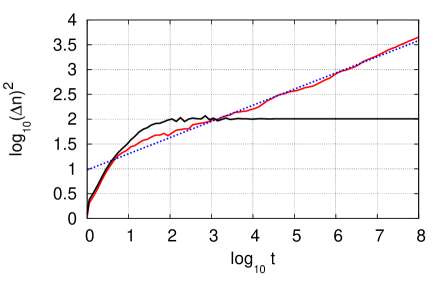
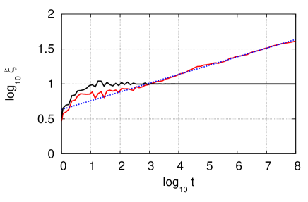
To characterize the properties of time evolution we compute one-site probability $w_{\bm{n}}=|\psi_{\bm{n}}|^{2}$, second moment of the probability distribution $(\Delta n)^{2}$ in 1D and $(\Delta R)^{2}=(\Delta n_{x})^{2}+(\Delta n_{y})^{2}$ in 2D, and the inverse participation ratio (IPR) $\xi=1/\sum_{\bm{n}}{w_{\bm{n}}}^{2}$ which gives an effective number of sites populated by the wave packet if all ${w_{\bm{n}}}^{2}$ probabilities are of the same order. To suppress fluctuations the quantities $(\Delta n)^{2}$, $(\Delta R)^{2}$, $\xi=1/\sum_{\bm{n}}{w_{\bm{n}}}^{2}$ are averaged over time intervals which are equally spaced in $\log t$. In addition the logarithms of these quantities are averaged over $N_{d}=10$ disorder realizations. The dependence on time is fitted by the algebraic dependencies $(\Delta n)^{2}\sim t^{\alpha_{1}}$, $(\Delta R)^{2}\sim t^{\alpha_{2}}$, $\xi\sim t^{\nu}$ with the exponents $\alpha_{1},\alpha_{1},\nu$.

The numerical results presented in Figs. 1,2 give values of exponents $\alpha_{1}=0.325\pm 0.003$ and $\nu=0.125\pm 0.001$. The value of $\alpha_{1}$ is in agreement with the data obtained in dls2008 where it was found that $\alpha_{1}=0.306\pm 0.002$ at $W=4$. Indeed, it should be noted that the standard deviation $\Delta\alpha_{1}\approx 0.014$ for fluctuations in the exponent $\alpha_{1}$ from one disorder realization to another dls2008 is larger than the the formal standard error of the fit of averaged data (with $\Delta\alpha_{1}\approx 0.003$). If all states inside the width $\Delta n$ are populated in a homogeneous way then we should have $(\Delta n)^{2}\sim\xi^{2}$ and $\alpha_{1}=2\nu$. The numerical data of Figs. 1,2 give this ratio to be $\alpha_{1}/2\nu=1.3$ instead of 1. This indicates that the probability inside the width $\Delta n$ is distributed in inhomogeneous way. It is possible that the spreading has certain multi-fractal properties that give deviations from usual relations between high moments. At the same time our data clearly confirm that the IPR grows in unlimited way with time (see Fig. 2). This is different from the claim presented in flach2008 . We attribute this difference to the fact that in flach2008 the data have been presented only for one disorder realization and no data for fits and their statistical accuracy have been given. At the same time the data of flach2008 for the second moment $(\Delta n)^{2}$ are consistent with the results presented here and in dls2008 .

Figure 3: (Color online) KNR data (5) for probability distribution $w_{n}$ at times $t=10^{3}$ (red/gray); $10^{6}$ (green/gray), $10^{9}$ (blue black) for $\beta=0$ (top panel with overlapped curves) with basis size $N=2^{10}$, for $\beta=0.03$ (middle panel) with the same basis size and for $\beta=1$ (bottom panel, curves are from bottom to top at $|n|\approx 200$ for time from $t=10^{3}$ to $10^{9}$) at $N=2^{11}$; here $k=3$, $T=2$.

Figure 4: (Color online) The spreading of the second moment $(\Delta n)^{2}$ with number of map iterations $t$ for the KNR model for the parameters of Fig. 3: $\beta=0$ (black curve), $N=2^{10}$; $\beta=0.03$ (dashed green/light gray curve), $N=2^{10}$ and $\beta=1$ (red/gray curve), $N=2^{11}$. The straight line shows the fit for $100\leq t\leq 10^{9}$ with the slope $\alpha_{1}=0.387\pm 0.003$.

Figure 5: (Color online) Same as in Fig. 5 for the IPR $\xi$ in the KNR model. The straight line shows the fit for $100\leq t\leq 10^{9}$ with the slope $\nu=0.210\pm 0.002$.

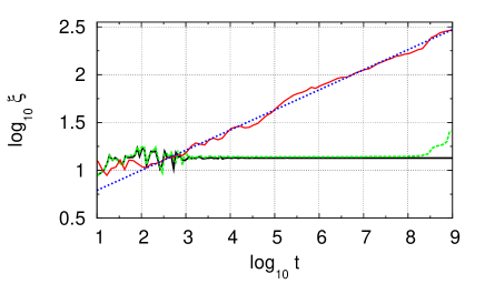
To obtain more results for larger times we also performed numerical simulations for the KNR model introduced in dls1993 . It time evolution is described by the map for the wave function:

$$\psi_{n}(t+1)=e^{-iT\hat{n}^{2}/2-i\beta|\psi_{n}|^{2}}e^{-ik\cos\hat{\theta}}\psi_{n}(t)\;,$$ (5)

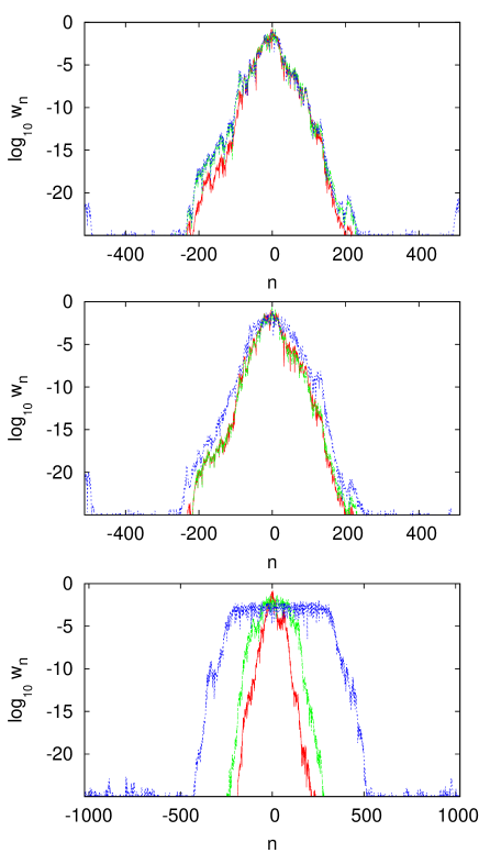
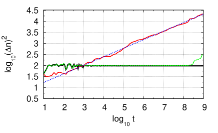
where $(\hat{n},\hat{\theta})$ are the conjugated operators with the commutation relation $[\hat{n},\hat{\theta}]=-i$ and $\psi$ is periodic in $\theta$. For $\beta=0$ this is the model of kicked rotator where all quasienergy eigenstates are exponentially localized with a localization length $l\approx k^{2}/2$ chirikov ; fishman . The propagation operator is similar to the one of (4) with $\Delta t=1$, due to that it is possible to perform $t=10^{9}$ map iterations of (5) for the same CPU time as for (4). The numerical results are presented in Figs.3-5.

These results show that unlimited spreading of probability over the sites $n$ takes place at moderate values of $\beta\sim 1$. The probability distribution over $n$ has a plateau followed by exponential tails, inside the plateau the probability is homogeneously distributed and the width of the plateau grows with time (see Fig. 3). The second moment of the distribution and the IPR grow algebraically in time with the exponents $\alpha_{1}=0.387\pm 0.003$ and $\nu=0.210\pm 0.002$ respectively (Figs. 4,5). In view of statistical fluctuations we consider that these values are in a good agreement with the theory estimates (see Eq. (3) and dls1993 ). The relation $\alpha_{1}=2\nu$ also works with a relatively weak deviation from the theory. For the KNR model the agreement with the theory is better than for the model (1). The possible reason is that in the KNR all linear eigenmodes have the same localization length $l\approx k^{2}/2$ while for the DANSE the localization length depends on the energy value inside the energy band that gives stronger statistical fluctuations and require longer times for the observation of the asymptotic algebraic growth. Also, it is possible that the stronger deviations of the exponent values from the theory in 1D DANSE model are related to the absence of good diffusive approximation for the 1D Anderson model while for the KNR model the diffusive approximation works rather well.

At small values of $\beta=0.03$ the probability distribution remains localized during enormously long times $t\leq 10^{8}$ but for larger time $t\sim 10^{9}$ the distribution grows slightly, also $\xi$ and $(\Delta n)^{2}$ are increased by a factor 2 and 3 respectively (see Figs. 3,4,5). It remains unclear if this is a fluctuation or if there is a very slow (logarithmic ?) spreading. In any case the behavior for small nonlinearity $\beta<\beta_{c}\sim 0.03$ is qualitatively different compared to the case of moderate values of $\beta\sim 1$ being in a qualitative agreement with the theoretical expectations.

IV Numerical results in 2D

Figure 6: (Color online) Probability distribution $w_{n_{x},n_{y}}$ inside the square $256\times 256$ at $W=10$ for $\beta=0$ (left column) and $\beta=1$ (right column) and time $t=10^{4}$ (bottom panels), $10^{6}$ (middle panels); probability is proportional to color with maximum at red/gray and zero at blue/black. Top panels show the decimal logarithm of the integrated probability $w_{n_{x}}=\sum_{n_{y}}w_{n_{x},n_{y}}$ for $-128\leq n_{x}\leq 127$ at $t=10^{4}$ (red/gray) and $10^{6}$ (black).

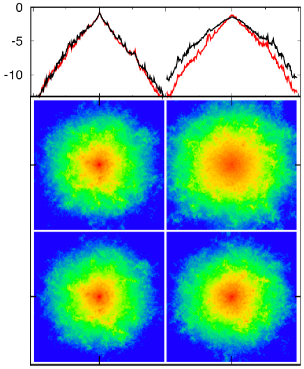
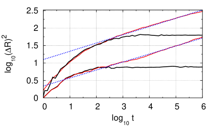
Here we present results for the model (1) in 2D. All results are averaged over $N_{d}=10$ disorder realisations. The time evolution of the probability distribution $w_{n_{x},n_{y}}$ is shown in Fig. 6 for $W=10$. At $\beta=0$ the probability is localized while at $\beta=1$ it slowly spreads over the lattice. The second moment of the space displacement $(\Delta R)^{2}=(\Delta n_{x})^{2}+(\Delta n_{y})^{2}$ as a function of time is shown in Fig. 7. The growth is well described by the algebraic dependence $(\Delta R)^{2}=Dt^{\alpha_{2}}$. The fit gives the values of the exponent $\alpha_{2}=0.236\pm 0.003$ for $W=10$ and $0.229\pm 0.003$ for $W=15$. Taking into account that the growth of $(\Delta R)^{2}$ is rather slow and that there are fluctuations related to disorder averaging the agreement of the exponent $\alpha_{2}$ with the theoretical value $\alpha=1/4$ (3) can be considered as rather good. In addition the value of $\alpha_{2}$ in 2D is decreased compared to the value $\alpha_{1}$ in 1D. Their ratio $\alpha_{2}/\alpha_{1}=0.233/0.325=0.717$ is rather close to the theoretical value $5/8$ given by Eq.(3). According to (3) the ratio $D(W=10)/D(W=15)=(l(W=10)/l(W=15))^{1/2}=((\Delta n(W=10))_{0}^{2}/(\Delta n(W=15))_{0}^{2}))^{1/4}\approx 1.9$ where $(\Delta n)_{0}^{2}$ are the values taken at $\beta=0$. From the data of Fig. 7 at $\beta=0$ we have this ratio to be 1.9 while from data at $\beta=1$ we obtain its value as 5 that can be considered as satisfactory taking into account all fluctuations.

Figure 7: (Color online) Average of the squared spreading $(\Delta R)^{2}$ as a function of time for two different values of the disorder strength $W=10$ (top red/gray and black curves) and $W=15$ (bottom red/gray and black curves) for $\beta=1$ (red/gray curves) and $\beta=0$ (black curves). The slopes of the straight line fits for $100\leq t\leq 10^{6}$ give $\alpha_{2}=0.236\pm 0.003$ for $W=10$ and $0.229\pm 0.003$ for $W=15$. The lattice size is as in Fig. 6.

The time dependence of the IPR $\xi$ is shown in Fig. 8. The fit gives the algebraic growth with the exponents $\nu=0.282\pm 0.002$ for $W=10$ and $\nu=0.247\pm 0.005$ for $W=15$ that is in a good agreement with the theoretical value $1/4$ (3). We note that in 2D the exponents $\alpha_{2}$ and $\nu$ become rather close. This indicates that multi-fractal effects become less pronounced in 2D.

Figure 8: (Color online) Same as in Fig. 7 but for the IPR $\xi$. The slopes of the straight line fit are $\nu=0.282\pm 0.002$ for $W=10$ (top red/gray and black curves) and $\nu=0.247\pm 0.005$ for $W=15$ (bottom red/gray and black curves); black curves are for $\beta=0$, red/gray curves are for $\beta=1$.

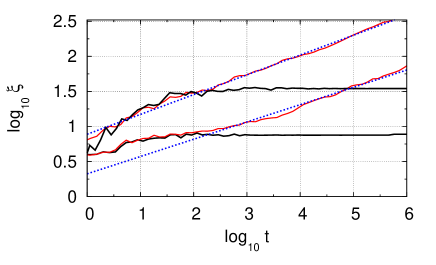
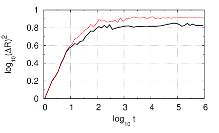
Finally, in Fig. 9 we present the comparison of the behaviors of linear system $\beta=0$ and the one at weak nonlinearity $\beta=0.033$. These data show that for $\beta<\beta_{c}$ the behaviors of the two systems are rather similar, for times explored in our numerical simulations, that is in agreement with the theoretical expectations described in Section II. According to our data $\beta_{c}>0.033$ in 2D.

Figure 9: (Color online) Average of the squared spreading $(\Delta R)^{2}$ as a function of time for for $\beta=0$ (black curve) and $\beta=0.033$ (red/gray curve) at $W=15$.

To characterize the nonlinear evolution of system (1) in an additional way we computed another characteristics which we call nonlinear fidelity defined as $f(t)=|\langle\tilde{\psi}_{n,m}(t)|\psi_{n,m}\rangle(t)|^{2}$, where $\tilde{\psi}_{n,m}(t)$ is a small perturbation of $\psi_{n,m}$ at $t=0$. For the linear system with $\beta=0$ the fidelity $f(t)$ remains constant during time evolution. However, for nonlinear dynamics $f(t)$ starts to depend on time. Indeed, the perturbation changes the nonlinear potential and the system starts to evolve with a slightly different effective Hamiltonian that leads to a decrease of fidelity. Such a behavior reminds the fidelity decay studied in systems of quantum chaos (see e.g. review prosen ). We note that recently the fidelity decay in the GPE has been studied in manfredi , however, there the amplitude of random potential was considered as a very small perturbation while in our case the disordered potential is strong and plays a dominant role. Also in manfredi the fidelity was considered for perturbation of potential while we consider the perturbation of nonlinear field that was not addressed in manfredi .

Figure 10: (Color online) Dependence of averaged $f(t)/f_{\rm max}$ as a function of the rescaled time $\Gamma t$ for $W=8$, $\beta=1$ and 7 different values of perturbed probability $0.001\leq\delta P\leq 0.03$. The average is done over $N_{d}=12$ disorder realizations. The straight line shows the dependence $f(t)/f_{\rm max}=\exp(-\Gamma t)$.

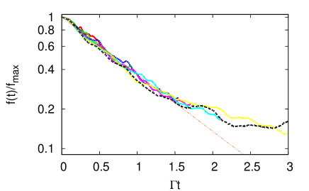
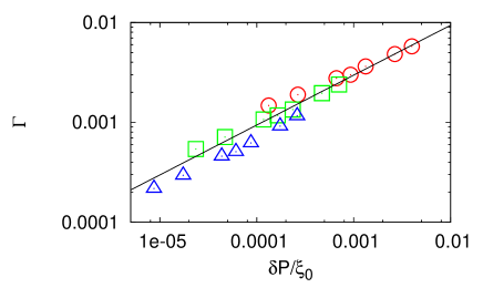
To study the properties of $f(t)$ we start at $t=0$ from one lattice state for $\psi$ while the state $\tilde{\psi}$ has a part $\delta P$ of total probability transferred to 8 nearby lattice sites (e.g. at $t=0$ for $\psi$ the total probability is at a certain lattice site, while for $\tilde{\psi}$ this site contains the probability $1-\delta P$ and nearby 8 sites have equal probabilities $\delta P/8$). For convenience we fit the decay of fidelity normalized by its maximal value $f_{max}$ by the exponential decay $f(t)/f_{max}=\exp(-\Gamma t)$ with a certain decay rate $\Gamma$. The value of $\Gamma$ is fixed by the condition that curves for various values of $\delta P$ are approximately superimposed on one scaling curve as it is shown for example in Fig. 10 for $W=8$ and $\beta=1$. The same procedure was done for other values of disorder $W$. The resulting dependence of $\Gamma$ on $\delta P$ and the average IPR $\xi_{0}$ at large times at $\beta=0$ is shown in Fig. 11. The data can be described by the dependence $\Gamma\sim(\delta P/\xi_{0})^{1/2}$. We interpret this in the following way: the perturbation$\delta P$ spreads over $\xi_{0}$ states and gives a modification of the nonlinear potential $\delta|\psi|^{2}\sim(\delta P/\xi_{0})^{1/2}$ that determines a typical transition frequency to other states leading to $\Gamma\sim\beta\delta|\psi|^{2}\sim\beta(\delta P/\xi_{0})^{1/2}$. A more detailed check of the functional dependence requires larger variation of $\xi_{0}$ that can be done in future studies.

Figure 11: (Color online) Dependence of the fidelity decay rate $\Gamma$ on rescaled perturbation $\delta P/\xi_{0}$ for $W=8$ (triangles), $10$ (squares), $15$ (circles). The straight line shows the algebraic dependence given by fit: $\Gamma=(\delta P/\xi_{0})^{\eta}$ with $\eta=0.486$.

Figure 12: (Color online) Rescaled fidelity decay as a function of time, for $W=8,\,\beta=1$ and values of $\delta P$ from 0.005 (top curve) to 0.7 (bottom curve); averaging is done over $N_{d}=12$ disorder realisations. At large $\delta P$ the behavior of $f(t)/f_{\rm max}$ becomes independent of $\delta P$. The straight line shows the decay with the saturated value of $\Gamma_{s}$: $f(t)/f_{max}=\exp(-\Gamma_{s}t)$.

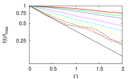
It is interesting to note that with the increase of $\delta P$ the growth of the decay rate $\Gamma$ becomes saturated and $\Gamma$ reaches its saturated value $\Gamma_{s}$ (see Fig. 12). The dependence of $\Gamma_{s}$ on $\xi_{0}$ is shown in Fig. 13. Except the strongly localized case at $W=15$ the dependence is satisfactorily described by $\Gamma_{s}\sim\beta/\xi_{0}$. This corresponds to the situation when the perturbation of nonlinear field is rather strong and the decay of fidelity is given by a typical nonlinear frequency shift $\delta\omega\sim\beta|\psi_{n}|^{2}\sim\beta/\xi_{0}$. Of course, this relation is valid on relatively short time scales used for investigation of fidelity decay (Figs. 10-13) when $|\psi_{n}|^{2}\sim\xi_{0}$. On a larger time scales the grows of $\xi(t)$ with time should be taken into account.

Figure 13: (Color online) Dependence of saturated decay rate $\Gamma_{s}$ (like in Fig. 12) on the IPR $\xi_{0}$ for $W=15,\,12,\,10,\,9,\,8$ (from left to right). The slope of the straight line fit is $-0.831\pm 0.0095$.

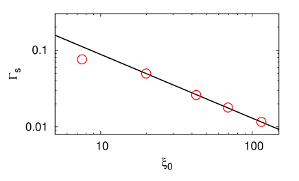
The nonlinear fidelity decay gives new additional characteristics of nonlinear field evolution on moderate time scales.

V Conclusions

The results of extensive numerical simulations presented above show that at moderate nonlinearity in disordered lattices with localized linear eigenmodes in 1D and 2D there is an algebraic spreading over the lattice with the number of populated sites growing as $\Delta n\propto t^{\nu}$ (see Eq. (3)). This spreading continues up to enormously large times $t=10^{9}$ while for the linear problem the localization takes place on a time scale $t_{loc}\sim 10$ or $100$. This result is in a satisfactory agreement with the previous studies dls1993 ; dls2008 . The numerical data are obtained on extremely large time scales (up to $t=10^{9}$ in dimensionless units) that are by 4 (Figs. 7,8) to 8 (Figs. 4,5) orders of magnitude larger than the time scale of Anderson localization (down to $t_{loc}=10$). This indicates that the numerical results demonstrate the real asymptotic regime of algebraic growth. Even if the numerical simulations do not allow to make rigorous conclusions about the asymptotic spreading at infinite times we think that the enormous difference between $t_{loc}$ scale and the computational times reached in our numerical simulations favors the conclusion that the presented numerical data give the real asymptotic behavior. The theoretical exponent of spreading $\nu=d/(3d+2)$ given by Eq. (3) is in a good agreement with the numerical data for the KNR model in 1D (5) and the 2D Anderson model (1) (see Figs. 4,5,7,8). For the 1D Anderson model (1) the numerical value of the exponent $\nu$ shows about 20-30% deviation from the theoretical value. We think that such a deviation should be attributed to a specific property of the 1D Anderson model which has no diffusive regime showing a direct transition from a ballistic dynamics to localization (see e.g. kramer1993 ). The data obtained for a weak nonlinearity with $\beta\leq 0.03$ show no spreading up to times $t=10^{6},10^{8}$ (see Fig. 9, Ref. dls2008 , Fig. 4, Fig. 5 respectively). A small spreading seeing in the KNR model at enormously large time $t=10^{9}$ may indicate that a very slow (logarithmic ?) spreading in time is not completely excluded and processes like the Arnold diffusion chirikov may be present. However, this spreading, even if present, is so slow that in global the presented numerical data can be considered as a confirmation of the theoretical expectation according to which for a typical initial state the localization is preserved at $\beta<\beta_{c}$. Our data indicate that $\beta_{c}\sim 1/30$. Indeed, the spreading behavior is qualitatively different for $\beta\sim 1$ and $\beta\sim 1/30$.

It is possible that such type of slow probability and energy spreading over disordered lattices may play an important role in complex molecules giving more rapid propagation of probability and energy along molecular chains compared to a simple diffusion produced by noise. It would be interesting to observe the nonlinear destruction of localization for BEC in disordered potential or for nonlinear waves in photonic lattices but this is rather hard task since very long observation times are required for that.

We thank A.S.Pikovsky for stimulating discussions, one of us (DLS) thanks the participants of the NLSE workshop at the Lewiner Institute at the Technion for useful discussions.

Note added: after the submission of this paper there appeared the preprint flacharx where the same nonlinear 1D Anderson model is investigated numerically and analytically.

References

- (1) P.W. Anderson, Phys. Rev. 109, 1492 (1958).
- (2) E. Akkermans and G. Montambaux, Mesoscopic Physics of Electrons and Photons, Cambridge Univ. Press, Cambridge (2007).
- (3) F. Dalfovo, S. Giorgini, L.P. Pitaevskii, and S. Strigani, Rev. Mod. Phys. 71, 463 (1999).
- (4) O. Morsch and M. Oberthaler, Rev. Mod. Phys. 78, 179 (2006).
- (5) L. Fallani, C.Fort, and M.Inguscio, arxiv:[0804.2888[cond-mat] (2008).
- (6) J.E. Lye, L. Fallani, M. Modugno, D.S. Wiersma, C. Fort, and M. Inguscio, Phys. Rev. Lett. 95, 070401 (2005).
- (7) D. Clément, A.F. Varón, M. Hugbart, J.A. Retter, P. Bouyer, L. Sanchez-Palencia, D.M.Gangardt, G.V.Shlyapnikov, and A. Aspect, Phys. Rev. Lett. 95, 170409 (2005).
- (8) C. Fort, L. Fallani, V. Guarrera, J.E. Lye, M. Modugno, D.S. Wiersma, and M. Inguscio, Phys. Rev. Lett. 95, 170410 (2005).
- (9) T.Schulte, S. Drenkelforth, J.Kruse, W.Ertmer, J. Arlt, K. Sacha, J.Zakrzewski, and M. Lewenstein, Phys. Rev. Lett. 95, 170411 (2005).
- (10) D. Clément, A.F. Varón, J.A. Retter, L. Sanchez-Palencia, A. Aspect, and P. Bouyer, New J. Phys. 8, 165 (2006).
- (11) C. Ryu, M.F. Andersen, A. Vaziri, M.B. d’Arcy, J.M. Grossman, K. Helmerson, and W.D. Phillips, Phys. Rev. Lett. 96, 160403 (2006).
- (12) G. Behinaein, V. Ramareddy, P. Ahmadi, and G.S. Summy, Phys. Rev. Lett. 97, 244101 (2006).
- (13) J. F. Kanem, S. Maneshi, M. Partlow, M. Spanner and A. M. Steinberg, Phys. Rev. Lett. 98, 083004 (2007).
- (14) B. V. Chirikov, Phys. Rep. 52, 263 (1979); B. V. Chirikov, F. M. Izrailev and D. L. Shepelyansky, Sov. Scient. Rev. C 2, 209 (1981); Physica 33D, 77 (1988); B. Chirikov and D. Shepelyansky, Scholarpedia 3(3):3550 (2008).
- (15) T. Schwartz, G. Bartal, S. Fishman, and M. Segev, Nature 446, 52 (2007).
- (16) Y. Lahini, A. Avidan, F. Pozzi, M. Sorel, R. Morandotti, D.N. Christodoulides, and Y. Silberberg, Phys. Rev. Lett. 100, 013906 (2008).
- (17) H. Cao, Waves in Random Media 13, R1 (2003).
- (18) S.A. Gredeskul and Y.S.Kivshar, Phys. Rep. 216, 1 (1992).
- (19) T. Paul, P. Schlagheck, P. Leboef, and N.Pavloff, Phys. Rev. Lett. 98, 210602 (2007).
- (20) F. Benvenuto, G. Casati, A.S.Pikovsky, and D.L.Shepelyansky, Phys. Rev. A 44, R3423 (1991).
- (21) D.L. Shepelyansky, Phys. Rev. Lett. 70, 1787 (1993).
- (22) N. Bilas and N. Pavloff, Phys. Rev. Lett. 95, 130403 (2005).
- (23) L. Sanchez-Palencia, D. Clément, P. Lugan, P. Bouyer, G.V.Shlyapnikov, and A. Aspect, Phys. Rev. Lett. 98, 210401 (2007).
- (24) G. Kopidakis, S. Komineas, S. Flach, and S. Aubry, Phys. Rev. Lett. 100, 084103 (2008).
- (25) A.S. Pikovsky and D.L. Shepelyansky, Phys. Rev. Lett. 100, 094101 (2008).
- (26) A. Dhar and J.L. Lebowitz, Phys. Rev. Lett. 100, 134301 (2008).
- (27) S.E. Skipetrov, and R. Maynard, Phys. Rev. Lett. 85, 736 (2000).
- (28) B. Shapiro, Phys. Rev. Lett. 99, 060602 (2007).
- (29) T. Wellens and B. Gremaud, Phys. Rev. Lett. 100, 033902 (2008).
- (30) S.E. Skipetrov, A. Minguzzi, B.A. van Tiggelen, and B. B.Shapiro, Phys. Rev. Lett. 100, 165301 (2008).
- (31) J. Frolich, T. Spencer, and C.E.Wayne, J. Stat. Phys. 42, 247 (1986).
- (32) G. Iooss, and G. James, Chaos 15, 015113 (2005).
- (33) O.V. Zhirov, G. Casati, and D.L. Shepelyansky, Phys. Rev. E 65, 026220 (2002); arXiv:cond-mat/0501188 (2005).
- (34) S. Fishman, Y.Krivopalov, and A. Soffer, J. Stat. Phys. bf 131, 843 (2008).
- (35) W.-M. Wang and Z.Zhang, preprint arXiv:0805.3520[math-ph] (2008).
- (36) J. Bourgain and W.-M. Wang, J. Eur. Math. Soc. 10, 1 (2008); preprint arXiv:0805.4632 [math.DS] (2008).
- (37) B. Kramer, and A. MacKinnon, Rep. Prog. Phys. 56, 1469 (1993).
- (38) D.L. Shepelyansky, Phys. Rev. Lett. 73, 2607 (1994).
- (39) P. Jacquod and D.L. Shepelyansky, Phys. Rev. Lett. 75, 3501 (1995).
- (40) B.V. Chirikov and D.L. Shepelyanskii, Sov. J. Nucl. Fiz. 36, 908 (1982) [Yader. Fiz. 36, 1563 (1982)].
- (41) S. Fishman, D. R. Grempel, and R. E. Prange, Phys. Rev. Lett. 49, 509 (1982).
- (42) T. Gorin, T. Prosen, T. H. Seligman and M. Znidaric, Phys. Rep. 435, 33 (2006).
- (43) G. Manfredi and P.-A.Hervieux, Phys. Rev. Lett. 100, 050405 (2008).
- (44) S. Flach, D.O. Krimer, and Ch. Skokos, preprint arXiv:0805.4693[cond-mat] (2008).